Sherlock: Sparse Hierarchical Embeddings for Visually-aware
One-class Collaborative Filtering

Abstract

Building successful recommender systems requires uncovering the underlying dimensions that describe the properties of items as well as users’ preferences toward them. In domains like clothing recommendation, explaining users’ preferences requires modeling the visual appearance of the items in question. This makes recommendation especially challenging, due to both the complexity and subtlety of people’s ‘visual preferences,’ as well as the scale and dimensionality of the data and features involved. Ultimately, a successful model should be capable of capturing considerable variance across different categories and styles, while still modeling the commonalities explained by ‘global’ structures in order to combat the sparsity (e.g. cold-start), variability, and scale of real-world datasets. Here, we address these challenges by building such structures to model the visual dimensions across different product categories. With a novel hierarchical embedding architecture, our method accounts for both high-level (colorfulness, darkness, etc.) and subtle (e.g. casualness) visual characteristics simultaneously.

1 Introduction

Identifying and understanding the dimensions of users’ opinions is a key component of any modern recommender system. Low-dimensional representations form the basis for Matrix Factorization methods, which model the affinity of users and items via their low-dimensional embeddings. In domains like clothing recommendation where the visual factors are largely at play, it is crucial to identify the visual dimensions of people’s opinions in order to model personalized preference most accurately.

In such domains, the visual appearance of the items are crucial side-signals that facilitate cold-start recommendation. However, uncovering visual dimensions directly from the images is particularly challenging as it involves handling semantically complicated and high-dimensional visual signals. In real-world recommendation data, items often come from a rich category hierarchy and vary considerably. Presumably there are dimensions that focus on globally-relevant visual rating facets (colorfulness, certain specific pattern types, etc.) across different items, as well as subtler dimensions that may have different semantics (in terms of the combination of raw features) for different categories. For instance, the combination of raw features that determine whether a coat is ‘formal’ might be totally different from those for a watch. Collars, buttons, pockets, etc. are at play in the former case, while features that distinguish digital from analogue or different strap types are key in the latter. Thus extracting visual dimensions requires a deep understanding of the underlying fine-grained variances.

Existing works address this task by learning a linear embedding layer (parameterized by a matrix) on top of the visual features extracted from product images with a pre-trained Deep Convolutional Neural Network (Deep CNN) He and McAuley (2016b); McAuley et al. (2015); He and McAuley (2016a). This technique has seen success for recommendation tasks from visually-aware personalized ranking (especially in cold-start scenarios), to discriminating the relationships between different items (complement, substitute, etc.). However, with a single embedding matrix shared by all items, such a model is only able to uncover ‘general’ visual dimensions, but is limited in its ability to capture subtler dimensions. Therefore the task of modeling the visual dimensions of people’s opinions is only partially solved.

In this paper, we propose an efficient sparse hierarchical embedding method, called Sherlock, to uncover the visual dimensions of users’ opinions on top of raw visual features (e.g. Deep CNN features extracted from product images). With a flexible distributed architecture, Sherlock is scalable and allows us to simultaneously learn both general and subtle dimensions, captured by different layers on the category hierarchy. More specifically, our main contributions include:

• We propose a novel hierarchical embedding method for uncovering visual dimensions. Our method directly facilitates personalized ranking in the one-class Collaborative Filtering setting, where only the ‘positive’ responses (purchases, clicks, etc.) of users are available.

• We quantitatively evaluate Sherlock on large e-comm-erce datasets: Amazon Clothing Shoes & Jewelry, etc. Experimental results demonstrate that Sherlock outperforms state-of-the-art methods in both warm-start and cold-start settings.

• We visualize the visual dimensions uncovered by Sherlock and qualitatively analyze the differences with state-of-the-art methods.

2 Related Work

One-class Collaborative Filtering. Pan et al. (2008) introduced the concept of One-Class Collaborative Filtering (OCCF) to allow Collaborative Filtering (CF) methods, especially Matrix Factorization (MF), to model users’ preferences in one-class scenarios where only positive feedback (purchases, clicks, etc.) is observed. This line of work includes point-wise models Hu et al. (2008); Pan et al. (2008) which implicitly treat non-observed interactions as ‘negative’ feedback. Such ideas were refined by Rendle et al. (2009) to develop a Bayesian Personalized Ranking (BPR) framework to optimize pair-wise rankings of positive versus non-observed feedback. BPR-MF combines the strengths of the BPR framework and the efficiency of MF and forms the basis of many state-of-the-art personalized OCCF methods (e.g. Pan and Chen (2013); Krohn-Grimberghe et al. (2012); He and McAuley (2016b); Zhao et al. (2014)).

Incorporating Side-Signals. Despite their success, MF-based methods suffer from cold-start issues due to the lack of observations to estimate the latent factors of new users and items. Making use of ‘side-signals’ on top of MF approaches can provide auxiliary information in cold-start settings while still maintaining MF’s strengths. Such signals include the content of the items themselves, ranging from the timbre and rhythm for music Wang et al. (2014); Koenigstein et al. (2011), textual reviews that encode dimensions of opinions McAuley and Leskovec (2013); Zhang et al. (2014a); Ling et al. (2014), or social relations Zhao et al. (2014); Jamali and Ester (2010); Pan and Chen (2013); Krohn-Grimberghe et al. (2012). Our work follows this line though we focus on a specific type of signal—visual features—which brings unique challenges when modeling the complex dimensions that determine users’ and items’ interactions.

Visually-aware Recommender Systems. The importance of using visual signals (i.e., product images) in recommendation scenarios has been stressed by previous works, e.g. Di et al. (2014); Goswami et al. (2011). State-of-the-art visually-aware recommender systems make use of high-level visual features of product images extracted from (pre-trained) Deep CNNs on top of which a layer of parameterized transformation is learned to uncover those “visual dimensions” that predict users’ actions (e.g. purchases) most accurately. Modeling this transformation layer is non-trivial as it is crucial to maximally capture the wide variance across different categories of items without introducing prohibitively many parameters into the model.

A recent line of work He and McAuley (2016b, a); He et al. (2016) makes use of a single parameterized embedding matrix to transform items from the CNN feature space into a low-dimensional ‘visual space’ whose dimensions (called ‘visual dimensions’) are those that maximally explain the variance in users’ decisions. While a simple parameterization, this technique successfully captures the common features among different categories, e.g. what characteristics make people consider a t-shirt or a shoe to be ‘colorful.’ But it is limited in its ability to model subtler variations, since each item is modeled in terms of a low-dimensional, global embedding. Here, we focus on building flexible hierarchical embedding structures that are capable of efficiently capturing both the common features and subtle variations across and within categories.

Taxonomy-aware Recommender Systems. There has been some effort to investigate ‘taxonomy-aware’ recommendation models, including earlier works extending neighborhood-based methods (e.g. Ziegler et al. (2004); Weng et al. (2008)) and more recent endeavors to extend MF using either explicit (e.g. Mnih (2012)) or implicit (e.g. Zhang et al. (2014b); Mnih and Teh (2012); Wang et al. (2015)) taxonomies. This work is related to ours, though does not consider the visual appearance of products as we do here.

3 The Sherlock Model

We are interested in learning visually-aware preference predictors from a large corpus of implicit feedback, i.e., the ‘one-class’ setting. Formally, let $\mathcal{U}$ and $\mathcal{I}$ be the set of users and items respectively. Each user $u\in\mathcal{U}$ has expressed positive feedback about a set of items $\mathcal{I}_{u}^{+}$. Each item $i\in\mathcal{I}$ is associated with a visual feature vector $f_{i}\in\mathbf{R}^{F}$ extracted from a pre-trained Deep CNN. For each item we are also given a path on a category hierarchy from the root node to a leaf category $\mathcal{C}_{i}$ (e.g. Clothing $\rightarrow$ Women’s Clothing $\rightarrow$ Shoes). Our objective is to build an efficient visually-aware preference predictor based on which a personalized ranking of the non-observed items (i.e., $\mathcal{I}\setminus\mathcal{I}_{u}^{+}$) is predicted for each user $u\in\mathcal{U}$.

3.1 The Basic Visually-aware Predictor

A visually-aware personalized preference predictor can be built on top of MF He and McAuley (2016b), which predicts the ‘affinity score’ between user $u$ and item $i$, denoted by $\widehat{x}_{u,i}$, by their interactions on visual and non-visual dimensions simultaneously:

$$\widehat{x}_{u,i}=\underbrace{\langle\overbrace{\theta_{u};\gamma_{u}}^{\text{user factors}},\overbrace{\theta_{i};\gamma_{i}}^{\text{item factors}}\rangle}_{\text{interactions between $u$ and $i$}}+\underbrace{\langle\vartheta,f_{i}\rangle}_{\text{visual bias of $i$}}+\beta_{i},$$ (1)

where user $u$’s preferences on visual and non-visual (latent) dimensions are represented by vectors $\theta_{u}\in\mathbf{R}^{K^{\prime}}$ and $\gamma_{u}\in\mathbf{R}^{K}$ respectively. Correspondingly, $\theta_{i}\in\mathbf{R}^{K^{\prime}}$ and $\gamma_{i}\in\mathbf{R}^{K}$ are two vectors encoding the visual and non-visual ‘properties’ of item $i$. The affinity between $u$ and $i$ is then predicted by computing the inner product of the two concatenated vectors. Item $i$ is also associated with an offset composed of two parts: visual bias captured by the inner product of $\vartheta$ and $f_{i}$, and the (non-visual) residue $\beta_{i}$.

3.2 Modeling the Visual Dimensions

The key to the above predictor is to model the visual dimensions of users’ opinions, which has seen success at tackling cold-start issues especially for domains like clothing recommendation where visual factors are at play. Instead of standard dimensionality reduction techniques like PCA, prior works have found it more effective to learn an embedding kernel (parameterized by a $K^{\prime}\times F$ matrix $\mathbf{E}$) to linearly project items from the raw CNN feature space to a low-dimensional ‘visual space’ He and McAuley (2016b, a). Critically, each dimension of the visual space encodes one visual facet that users consider; these facets $\theta_{i}$ are thus modeled by $\theta_{i}=\mathbf{E}f_{i}$, i.e., all $\theta_{i}$’s are parameterized by a single matrix $\mathbf{E}$.

For each visual dimension $D$, the above technique computes the extent to which an item $i$ exhibits this particular visual rating facet (i.e., the ‘score’ $\theta_{i}^{(D)}$) by the inner product

$$\theta_{i}^{(D)}=\langle\mathbf{E}^{(D)},f_{i}\rangle,$$ (2)

where $\mathbf{E}^{(D)}$ is the $D$-th row of $\mathbf{E}$. Despite its simple form, the embedding layer is able to uncover visual dimensions that capture ‘global’ features (e.g. colorfulness, a specific type of pattern) across different items. However, in settings where items are organized in a rich category hierarchy, such a single-embedding method can only partially solve the task of modeling visual preferences as dimensions that capture the subtle and wide variances across different categories are ignored. For example, the combination of raw features that determine whether a shirt is casual (such as a zipper and short sleeves) might be quite different from those for a shoe. Thus to extract the ‘scores’ on a visual dimension indicating casualness, each category may require a different parameterization.

It is the above properties that motivate us to use category-dependent structures to extract different visual embeddings for each category of item.

3.3 Sparse Hierarchical Embeddings

Variability is pervasive in real-world datasets; this is especially true in e-commerce scenarios where the items from different parts of a category hierarchy may vary considerably.

A simple idea would be to learn a separate embedding kernel for each (sub-) category to maximally capture the fine-grained variance. However, this would introduce prohibitively many parameters and would thus be subject to overfitting. For instance, the Amazon Women’s Clothing dataset with which we experiment has over 100 categories which would require millions of parameters just to model the embeddings themselves. Our key insight is that the commonalities among nodes sharing common ancestors mean that there would be considerable redundancy in the above scheme, which can be exploited with efficient structures. This inspires us to develop a distributed architecture—a flexible hierarchical embedding model—in order to simultaneously account for the commonalities and variances efficiently.

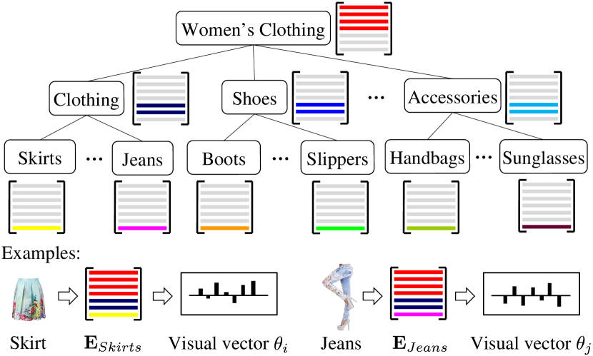
Figure 1: Illustration of the high-level idea of Sherlock. Each layer is associated with a segment of the embedding matrix, which is instantiated at each node on this layer. The embedding matrix at each leaf node is a concatenation/stack of the segments along the root-to-leaf path. (Here we demonstrate allocating $K^{\prime}=7$ visual dimensions with a 4:2:1 split on the hierarchy $\Psi$.)

Note that each row in the $K^{\prime}\times F$ embedding matrix $\mathbf{E}$ is used to extract a specific visual dimension. Let $\Psi$ denote the category hierarchy and $h_{\Psi}$ its height, the high-level idea is to partition the $K^{\prime}$ row indices of the embedding matrix into $h_{\Psi}$ segments such that each segment is associated with a specific layer on $\Psi$. For each layer, the associated segment is instantiated with an independent copy at each node which is used to extract the corresponding visual dimensions for all items in the subtree rooted with the node.

Figure 1 demonstrates a concrete example of extracting $K^{\prime}=7$ visual dimensions for the Amazon Women’s Clothing dataset. Here we show the top 3 layers of the hierarchy (i.e., $h_{\Psi}=3$); handling deep and complex hierarchies will be discussed later. In this example, layers 0, 1, and 2 are associated with segment $S_{0}=[0,1,2,3]$, $S_{1}=[4,5]$, and $S_{2}=[6]$ respectively. The $4\times F$ matrix associated with the root node will be used to extract the first 4 visual dimensions (i.e., $0$, $1$, $2$, $3$) for all items in the dataset. While the $2\times F$ matrices attached to the second-level nodes (i.e. Clothing, Shoes, etc.) are used to extract visual dimensions $4$ and $5$ for items in the corresponding subtrees. Finally, the $1\times F$ matrices on the bottom layer are used to extract dimension $6$ for each of the fine-grained categories (i.e., Skirts, Jeans, Boots, etc.).

Finally, each leaf node of $\Psi$ is associated with a full $K^{\prime}\times F$ embedding matrix, which is the concatenation/stacking of all the segment instances along the root-to-leaf path. Formally, let $(\mathcal{C}_{i}^{(1)}$, …, $\mathcal{C}_{i}^{(h_{\Psi})})$ be the root-to-leaf path of item $i$ on $\Psi$, and $S_{i}^{(l)}$ the segment of the embedding matrix associated with node $C_{i}^{(l)}$ on layer $l$. The full embedding matrix associated with the leaf node $\mathcal{C}_{i}^{(h_{\Psi})}$ is:

$$\mathbf{E}_{C_{i}^{(h_{\Psi})}}=\begin{bmatrix}\text{{-----}}~{}~{}S_{i}^{(1)}~{}~{}\text{{-----}}\\ \text{{-----}}~{}~{}S_{i}^{(2)}~{}~{}\text{{-----}}\\ \cdots\\ \text{{-----}}~{}~{}S_{i}^{(h_{\Psi})}\text{{-----}}\\ \end{bmatrix}_{K^{\prime}\times F}.$$

Then the ‘visual properties’ of item $i$ (i.e., $\theta_{i}$) are computed by

$$\theta_{i}=\mathbf{E}_{C_{i}^{(h_{\Psi})}}f_{i}.$$ (3)

For example, in Figure 1 the embedding matrix for the ‘Skirts’ node ($\mathbf{E}_{Skirts}$) consists of 4 rows inherited from the root, 2 rows from its parent ‘Clothing,’ and 1 row of its own. Each skirt item $i$ in the dataset will be projected to the visual space by $\mathbf{E}_{\mathit{Skirts}}f_{i}$.

Note that parameters attached to the ancestor are shared by all its descendants and capture more globally-relevant visual dimensions (e.g. colorfulness), while the more fine-grained dimensions (e.g. a specific style type) are captured by descendants on lower levels. This ‘sparse’ structure enables Sherlock to simultaneously capture multiple levels of dimensions with different semantics at a low cost.

The distributed architecture of Sherlock allows tuning the partition schemes of the $K^{\prime}$ visual dimensions to trade off the expressive power and the amount of free parameters introduced. Allocating more dimensions to higher layers can reduce the number of parameters, and the opposite will enhance the ability to capture more fine-grained characteristics. Note that Sherlock can capture the single-embedding model as a special case if it allocates all $K^{\prime}$ dimensions to the root node, i.e., use a $K^{\prime}:0:\ldots:0$ split.

Imbalanced Hierarchies. Sherlock is able to handle imbalanced category hierarchies. Let $\hbar$ be the length of the shortest path on an imbalanced hierarchy. Sherlock only assigns segments to layers higher than $\hbar$, using the same scheme as described before. In this way, the unbalanced hierarchy can be seen as being ‘reduced’ to a balanced one. Note that (1) real-world category hierarchies (such as Amazon’s catalogs) usually are not severely imbalanced, and (2) experimentally Sherlock does not need to go deep down the hierarchy to perform very well (as we show later), presumably because data get increasingly sparser when diving deeper.

3.4 Learning the Model

Bayesian Personalized Ranking (BPR) is a state-of-the-art framework to directly optimize the personalized ranking $>_{u}$ for each user $u$ Rendle et al. (2009). Assuming independence of users and items, it optimizes the maximum a posterior (MAP) estimator of the model parameters $\Theta$:

$$\operatorname*{arg\,max}_{\Theta}=\ln\prod_{u\in\mathcal{U}}\prod_{i\in\mathcal{I}_{u}^{+}}\prod_{j\notin\mathcal{I}_{u}^{+}}p(i>_{u}j|\Theta)~{}p(\Theta),$$ (4)

where the pairwise ranking between a positive ($i$) and a non-positive ($j$) item $p(i>_{u}j|\Theta)$ is estimated by a logistic function $\sigma(\widehat{x}_{u,i}-\widehat{x}_{u,j})$.

Let $\mathbf{E}^{*}$ denote the set of embedding parameters associated with the hierarchy $\Psi$, then the full set of parameters of Sherlock becomes $\Theta=\{\beta_{i},\gamma_{i},\gamma_{u},\theta_{u},\vartheta,\mathbf{E}^{*}\}$. Using stochastic gradient ascent, first we uniformly sample a user $u$ as well as a positive/non-positive pair $(i,j)$, and then the learning procedure updates parameters as follows:

$$\Theta\leftarrow\Theta+\alpha\cdot(\sigma(\widehat{x}_{u,j}-\widehat{x}_{u,i})\frac{\partial(\widehat{x}_{u,i}-\widehat{x}_{u,j})}{\partial\Theta}-\lambda_{\Theta}\Theta),$$ (5)

where $\alpha$ represents the learning rate and $\lambda_{\Theta}$ is a regularization hyperparameter tuned with a held-out validation set.

Complexity Analysis. Here we mainly compare Sherlock against the single-embedding model. For a sampled triplet $(u,i,j)$, both methods require $O(K^{\prime}\times F+K)$ to compute $\widehat{x}_{u,i}-\widehat{x}_{u,j}$. Next, computing the partial derivatives for $\beta_{i}$, $\gamma_{i}$, $\gamma_{u}$, $\theta_{u}$, and $\vartheta$ take $O(1)$, $O(K)$, $O(K)$, $O(K^{\prime})$, and $O(F)$ respectively. Note that both models take $O(K^{\prime}\times F)$ for updating the embedding parameters due to the amount of parameters involved. In summary, Sherlock as well as the single-embedding model take $O(K^{\prime}\times F+K)$ for updating a sampled triple.

4 Experiments

In this section, we conduct experiments on real-world data-sets to evaluate the performance of Sherlock and visualize the hierarchical visual dimensions it uncovers.

Table 1: Dataset statistics

Dataset	#users ($|\mathcal{U}|$)	#items ($|\mathcal{I}|$)	#feedback
Men’s Clothing	1,071,567	220,478	1,554,834
Women’s Clothing	1,525,979	465,318	2,634,336
Full Clothing	2,948,860	1,057,034	5,338,520

4.1 Datasets

We are interested in evaluating our method on the largest datasets available. To this end, we adopted the Amazon dataset introduced by McAuley et al. (2015). In particular, we consider the Clothing Shoes & Jewelry dataset, since (1) clothing recommendation is a task where visual signals are at play, and (2) visual features have proven to be highly successful at addressing recommendation tasks on this dataset. Thus it is a natural choice for comparing our method against these previous models. Additionally, we also evaluate all methods on its two largest subcategories—Men’s and Women’s Clothing & Accessories. Statistics of these three datasets are shown in Table 1. For simplicity, in this paper we denote them as Men’s Clothing, Women’s Clothing, and Full Clothing respectively.

Category Tree. There is a category tree associated with each of our clothing datasets. Figure 1 demonstrates part of the hierarchy associated with Women’s Clothing. On this hierarchy, we have 10 second-level categories (Clothing, Shoes, Watches, Jewelry, etc.), and 106 third-level categories (e.g. Jeans, Pants, Skirts, etc. under the Clothing category).

Visual Features. Following the setting from previous works He and McAuley (2016b, a); McAuley et al. (2015), we employ the Deep CNN visual features extracted from the Caffe reference model Jia et al. (2014), which implements the architecture comprising 5 convolutional layers and 3 fully-connected layers Krizhevsky et al. (2012). See McAuley et al. (2015) for more details. In this experiment, we take the output of the second fully-connected layer FC7 to obtain a visual feature vector $f_{i}$ of $F=4096$ dimensions.

4.2 Evaluation Protocol

Here we mainly follow the leave-one-out protocol used by He and McAuley (2016b); Rendle et al. (2009), i.e., for each user $u$ we randomly sample a positive item $\mathcal{V}_{u}\in\mathcal{I}_{u}^{+}$ for validation and another $\mathcal{T}_{u}\in\mathcal{I}_{u}^{+}$ for testing. The remaining data is then used for training. Finally, all methods are evaluated in terms of the quality of the predicted personalized ranking using the average AUC (Area Under the ROC curve) metric:

$$\mathit{AUC}=\frac{1}{|\mathcal{U}|}\sum_{u\in\mathcal{U}}\frac{1}{|\mathcal{I}\setminus\mathcal{I}_{u}^{+}|}\sum_{j\in\mathcal{I}\setminus\mathcal{I}_{u}^{+}}\mathbf{1}(\widehat{x}_{u,\mathcal{T}_{u}}>\widehat{x}_{u,j}),$$ (6)

where $\mathbf{1}(\cdot)$ is the indicator function and the evaluation goes through the pair set of each user $u$.

All our experiments were conducted on a single desktop machine with 4 cores (3.4GHz) and 32GB memory. In all cases, we use grid-search to tune the regularization hyperparameters to obtain the best performance on the validation set and report the corresponding performance on the test set.

4.3 Baselines

We mainly compare our approach against BPR-based ranking methods, which are known to have state-of-the-art performance for implicit feedback dataset. The baselines we include for evaluation are:

• Random (RAND): This baseline ranks all items randomly for each user $u$.

• BPR-MF: Introduced by Rendle et al. (2009), this baseline is the state-of-the-art method for personalized ranking in OCCF settings. It takes the standard Matrix Factorization Ricci et al. (2011) as the preference predictor.

• Visual-BPR (VBPR): Built upon the BPR-MF model, it uncovers visual dimensions on top of Deep CNN features with a single embedding matrix He and McAuley (2016b). This is a state-of-the-art visually-aware model for the task though.

• VBPR-C: This baseline makes use of category tree to extend VBPR by associating a bias term to each fine-grained category on the hierarchy.

In summary, these baselines are designed to demonstrate (1) the strength of state-of-the-art visually-unaware method on our datasets (i.e., BPR-MF), (2) the effect of using the visual signals and modeling those visual dimensions (i.e., VBPR), and (3) the improvement of using the category tree signal to improve VBPR in a relatively straightforward manner (i.e., VBPR-C).

4.4 Performance and Quantitative Analysis

For each dataset, we evaluate all methods with two settings: Warm-start and Cold-start. The former focuses on measuring the overall ranking performance, while the latter the capability to recommend cold-start items in the system. Following the protocol used by He and McAuley (2016b), the Warm-start evaluation is implemented by computing the average AUC on the full test set, while Cold-start evaluates by only keeping the cold items in the test set, i.e., those that appeared fewer than five times in the training set.

For fair comparisons, all BPR-based methods use 20 rating dimensions. For simplicity, VBPR, VBPR-C, and Sherlock all adopt a 10:10 split, i.e., $K=10$ latent plus $K^{\prime}=10$ visual dimensions. To evaluate the performance of Sherlock, we use three different allocation schemes for the 10 visual dimensions, denoted by (e1), (e2), and (e3) respectively. Table 2 summarizes the detailed dimension allocation of each scheme for each of the three datasets. For Men’s and Women’s Clothing, all three schemes allocate the 10 visual dimensions to the top 3 layers on the category hierarchy. In contrast, visual dimensions are allocated to the top 4 layers for Full Clothing as it is larger in terms of both size and variance.

Table 2: Different evaluation schemes to allocate 10 visual dimensions. More visual dimensions are distributed to lower layers on the hierarchy in the order of (e1) $\Rightarrow$ (e2) $\Rightarrow$ (e3).

Scheme	Full Clothing	Men’s	Women’s
(e1)	6:2:1:1	7:2:1	7:2:1
(e2)	4:3:2:1	5:3:2	5:3:2
(e3)	2:3:3:2	3:4:3	3:4:3

Note that comparison between Sherlock and VBPR using the same amount of embedding parameters would be unfair for VBPR, as in that case VBPR would have to use a larger value of $K^{\prime}$ and would thus need to learn more parameters for $\theta_{u}$ and would be subject to overfitting.

Table 3 shows the average AUC of all methods achieved on our three datasets. The main findings from this table can be summarized as follows:

Table 3: AUC on the test set (total number of dimensions is set to 20). (e1), (e2) and (e3) correspond to the three evaluation schemes in Table 2. The best performing method in each case is boldfaced.

Dataset	Setting	(a)	(b)	(c)	(d)	(e1)	(e2)	(e3)	improvement
		RAND	BPR-MF	VBPR	VBPR-C	Sherlock	Sherlock	Sherlock	e vs. c	e vs. best
Full Clothing	Warm-start	0.5012	0.6134	0.7541	0.7552	0.7817	0.7842	0.7868	4.3%	4.2%
	Cold-start	0.4973	0.5026	0.6996	0.7002	0.7272	0.7400	0.7375	5.8%	5.7%
Men’s Clothing	Warm-start	0.4967	0.5937	0.7156	0.7161	0.7297	0.7341	0.7364	2.9%	2.8%
	Cold-start	0.4993	0.5136	0.6599	0.6606	0.6774	0.6861	0.6889	4.4%	4.3%
Women’s Clothing	Warm-start	0.4989	0.5960	0.7336	0.7339	0.7464	0.7476	0.7519	2.5%	2.5%
	Cold-start	0.4992	0.4899	0.6725	0.6726	0.6910	0.6960	0.7008	4.2%	4.2%

1. Visually-aware methods (VBPR, VBPR-C, and Sherlock) outperform BPR-MF significantly, which proves the usefulness of visual signals and the efficacy of the Deep CNN features.

2. VBPR-C does not significantly outperform VBPR, presumably because the category signals are already (at least partially) encoded by those visual features. This suggests that improving VBPR requires more creative ways to leverage such signals.

3. Sherlock predicts most accurately amongst all methods in all cases (up to 5.7%) especially for datasets with larger variance (i.e., Full Clothing) and in cold-start settings, which shows the effectiveness of using our novel hierarchical embedding architecture.

4. As we ‘offload’ more visual dimensions to lower layers on the hierarchy (i.e., (e1) $\Rightarrow$ (e2) $\Rightarrow$ (e3)), performance becomes increasingly better. This indicates the stability of Sherlock as well as the benefits from capturing category-specific semantics.

4.5 Training Efficiency

Each iteration of the stochastic gradient descent procedure consists of sampling training triples $(u,i,j)$ with the size of the training corpus. In Figure 2 we demonstrate the accuracy on the test set (Warm-start setting) of all visually-aware methods as the number of training iterations increases. As shown by the figure, Sherlock with three allocation schemes can all converge reasonably fast. As analyzed in Section 3, our methods share the same time complexity with VBPR, and experimentally both are able to finish learning the parameters within a couple of hours.

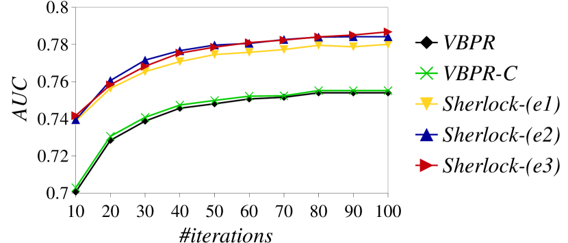
Figure 2: Comparison of visually-aware methods with number of training iterations on Full Clothing dataset.

4.6 Visualization of Visual Dimensions

Next we qualitatively demonstrate the visual dimensions revealed by Sherlock. To achieve this goal, we take our model trained on Men’s Clothing (10 visual dimensions with a split of 5:3:2) and rank all items on each visual dimension $D$ as follows: $\operatorname*{arg\,max}_{i}\theta_{i}^{(D)},$ i.e., to find items that maximally exhibit each dimension.

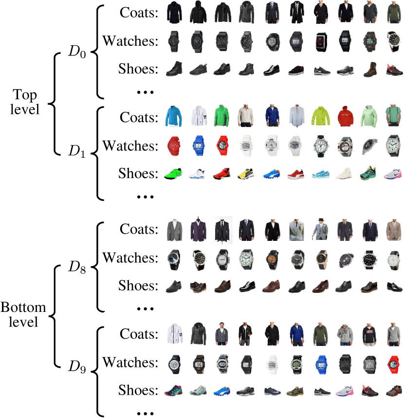
Figure 3: Demonstration of four visual dimensions uncovered by Sherlock on Men’s Clothing. Top-level dimensions $D_{0}$ and $D_{1}$ appear to capture ‘general’ notions (darkness and brightness); while bottom-level dimensions $D_{8}$ and $D_{9}$ capture subtler notions (business and casualness), which requires the ability to model category-specific semantics.

In Figure 3 we demonstrate four example dimensions, two associated with the top layer ($D_{0},D_{1}$), and the rest the bottom layer ($D_{8},D_{9}$). For each of these dimensions, we show the top-ranked items in a few of the bottom-level categories—Coats, Watches, and Shoes. We make the following observations from Figure 3.

Sherlock produces meaningful visual dimensions, each of which seems to capture a human notion. For example, dimensions $D_{0}$ and $D_{8}$ capture the notions of ‘dark’ and ‘formality’ respectively, though items are from different categories and vary considerably in aspects like shape and category-specific features.

As expected, Sherlock captures both globally-relevant and subtle dimensions. Top-level dimensions $D_{0}$ and $D_{1}$ are capturing the notions of darkness and brightness respectively, features which are applicable to all categories. While the bottom-level dimensions $D_{8}$ and $D_{9}$ are capturing the subtler notions of formality and casualness, which requires a deep understanding of category-specific semantics. For example, to extract the ‘business’ dimension ($D_{8}$), attributes like collar and button are at play for the Coats category, while features that distinguish digital from analogue or strap types are key for the Watches category.

Note the single-embedding model only uncovers dimensions like those captured by the top-level on our hierarchy. The strength of Sherlock in exploiting the commonalities and variances of items and uncovering dimensions makes it a successful method in addressing the recommendation task.

5 Conclusion

Uncovering rating dimensions and modeling user-item interactions upon them are key to building a successful recommender system. In this paper, we proposed a sparse hierarchical embedding method, Sherlock, that simultaneously reveals globally-relevant and subtle visual dimensions efficiently. We evaluated Sherlock for personalized ranking tasks in the one-class setting and found it to significantly outperform state-of-the-art methods on real-world datasets.

References

- Di et al. [2014] Wei Di, Neel Sundaresan, Robinson Piramuthu, and Anurag Bhardwaj. Is a picture really worth a thousand words?:-on the role of images in e-commerce. In WSDM, pages 633–642, 2014.
- Goswami et al. [2011] Anjan Goswami, Naren Chittar, and Chung H Sung. A study on the impact of product images on user clicks for online shopping. In WWW, pages 45–46, 2011.
- He and McAuley [2016a] Ruining He and Julian McAuley. Ups and downs: Modeling the visual evolution of fashion trends with one-class collaborative filtering. In WWW, 2016.
- He and McAuley [2016b] Ruining He and Julian McAuley. VBPR: visual bayesian personalized ranking from implicit feedback. In AAAI, 2016.
- He et al. [2016] Ruining He, Chunbin Lin, and Julian McAuley. Fashionista: A fashion-aware graphical system for exploring visually similar items. In WWW, 2016.
- Hu et al. [2008] Yifan Hu, Yehuda Koren, and Chris Volinsky. Collaborative filtering for implicit feedback datasets. In ICDM, pages 263–272, 2008.
- Jamali and Ester [2010] Mohsen Jamali and Martin Ester. A matrix factorization technique with trust propagation for recommendation in social networks. In RecSys, pages 135–142, 2010.
- Jia et al. [2014] Yangqing Jia, Evan Shelhamer, Jeff Donahue, Sergey Karayev, Jonathan Long, Ross Girshick, Sergio Guadarrama, and Trevor Darrell. Caffe: Convolutional architecture for fast feature embedding. In MM, pages 675–678, 2014.
- Koenigstein et al. [2011] Noam Koenigstein, Gideon Dror, and Yehuda Koren. Yahoo! music recommendations: modeling music ratings with temporal dynamics and item taxonomy. In RecSys, pages 165–172, 2011.
- Krizhevsky et al. [2012] Alex Krizhevsky, Ilya Sutskever, and Geoffrey E Hinton. Imagenet classification with deep convolutional neural networks. In NIPS, pages 1097–1105, 2012.
- Krohn-Grimberghe et al. [2012] Artus Krohn-Grimberghe, Lucas Drumond, Christoph Freudenthaler, and Lars Schmidt-Thieme. Multi-relational matrix factorization using bayesian personalized ranking for social network data. In WSDM, pages 173–182, 2012.
- Ling et al. [2014] Guang Ling, Michael R Lyu, and Irwin King. Ratings meet reviews, a combined approach to recommend. In RecSys, pages 105–112, 2014.
- McAuley and Leskovec [2013] Julian McAuley and Jure Leskovec. Hidden factors and hidden topics: understanding rating dimensions with review text. In RecSys, pages 165–172, 2013.
- McAuley et al. [2015] Julian McAuley, Christopher Targett, Qinfeng Shi, and Anton van den Hengel. Image-based recommendations on styles and substitutes. In SIGIR, pages 43–52, 2015.
- Mnih and Teh [2012] Andriy Mnih and Yee W Teh. Learning label trees for probabilistic modeling of implicit feedback. In NIPS, pages 2816–2824, 2012.
- Mnih [2012] Andriy Mnih. Taxonomy-informed latent factor models for implicit feedback. In KDD Cup, pages 169–181, 2012.
- Pan and Chen [2013] Weike Pan and Li Chen. GBPR: group preference based bayesian personalized ranking for one-class collaborative filtering. In IJCAI, pages 2691–2697, 2013.
- Pan et al. [2008] Rong Pan, Yunhong Zhou, Bin Cao, Nathan N Liu, Rajan Lukose, Martin Scholz, and Qiang Yang. One-class collaborative filtering. In ICDM, pages 502–511, 2008.
- Rendle et al. [2009] Steffen Rendle, Christoph Freudenthaler, Zeno Gantner, and Lars Schmidt-Thieme. BPR: Bayesian personalized ranking from implicit feedback. In UAI, pages 452–461, 2009.
- Ricci et al. [2011] Francesco Ricci, Lior Rokach, Bracha Shapira, and Paul Kantor. Recommender systems handbook. Springer US, 2011.
- Wang et al. [2014] Xinxi Wang, Yi Wang, David Hsu, and Ye Wang. Exploration in interactive personalized music recommendation: a reinforcement learning approach. ACM Transactions on Multimedia Computing, Communications, and Applications, 11(1), 2014.
- Wang et al. [2015] Suhang Wang, Jiliang Tang, Yilin Wang, and Huan Liu. Exploring implicit hierarchical structures for recommender systems. In IJCAI, pages 1813–1819, 2015.
- Weng et al. [2008] Li-Tung Weng, Yue Xu, Yuefeng Li, and Richi Nayak. Exploiting item taxonomy for solving cold-start problem in recommendation making. In ICTAI, pages 113–120, 2008.
- Zhang et al. [2014a] Yongfeng Zhang, Guokun Lai, Min Zhang, Yi Zhang, Yiqun Liu, and Shaoping Ma. Explicit factor models for explainable recommendation based on phrase-level sentiment analysis. In SIGIR, pages 83–92, 2014.
- Zhang et al. [2014b] Yuchen Zhang, Amr Ahmed, Vanja Josifovski, and Alexander Smola. Taxonomy discovery for personalized recommendation. In WSDM, pages 243–252, 2014.
- Zhao et al. [2014] Tong Zhao, Julian McAuley, and Irwin King. Leveraging social connections to improve personalized ranking for collaborative filtering. In CIKM, pages 261–270, 2014.
- Ziegler et al. [2004] Cai-Nicolas Ziegler, Georg Lausen, and Lars Schmidt-Thieme. Taxonomy-driven computation of product recommendations. In CIKM, pages 406–415, 2004.