Dynamical model reduction method for solving parameter-dependent dynamical systems thanks: This work was supported by the french research group GDR MoMaS.

Marie BILLAUD-FRIESS222Ecole Centrale de Nantes, GeM, UMR CNRS 6183, France.333Corresponding author (marie.billaud-friess@ec-nantes.fr). and Anthony NOUY222Ecole Centrale de Nantes, GeM, UMR CNRS 6183, France.
Abstract

We propose a projection-based model order reduction method for the solution of parameter-dependent dynamical systems. The proposed method relies on the construction of time-dependent reduced spaces generated from evaluations of the solution of the full-order model at some selected parameters values. The approximation obtained by Galerkin projection is the solution of a reduced dynamical system with a modified flux which takes into account the time dependency of the reduced spaces. An a posteriori error estimate is derived and a greedy algorithm using this error estimate is proposed for the adaptive selection of parameters values. The resulting method can be interpreted as a dynamical low-rank approximation method with a subspace point of view and a uniform control of the error over the parameter set.

1 Introduction

Parameter-dependent equations are considered in many problems of scientific computing such as optimization, control or uncertainty quantification. For complex numerical models, model order reduction methods are usually required for an efficient estimation of the solution for many values of the parameters (multi-query context). Classical model order reduction methods for parameter-dependent equations are the Reduced Basis (RB) method [20], the Proper Orthogonal Decomposition (POD) method [33] or the Proper Generalized Decomposition (PGD) method [26]. These methods can be interpreted as low-rank approximation methods with different constructions of the approximation for different controls of the error over the parameter set (uniform control for RB or control in mean-square sense for POD and PGD, see, e.g., [27]) .

This paper is concerned with the solution of parameter-dependent non-autonomous dynamical systems of the form

{𝒖(t,𝝃)=𝒇(𝒖(t,𝝃),t,𝝃),𝒖(0,𝝃)=𝒖0(𝝃),\left\{\begin{aligned} \boldsymbol{u}^{\prime}(t,\boldsymbol{\xi})&=\boldsymbol{f}(\boldsymbol{u}(t,\boldsymbol{\xi}),t,\boldsymbol{\xi}),\\ \boldsymbol{u}(0,\boldsymbol{\xi})&=\boldsymbol{u}^{0}(\boldsymbol{\xi}),\end{aligned}\right. (1)

where the flux 𝒇𝒇\boldsymbol{f} and initial condition depend on some parameters 𝝃𝝃\boldsymbol{\xi} with values in a parameter set 𝚵𝚵\boldsymbol{\Xi}. The solution 𝒖(t,𝝃)𝒖𝑡𝝃\boldsymbol{u}(t,\boldsymbol{\xi}) belongs to the high-dimensional state space X=d𝑋superscript𝑑X=\mathbb{R}^{d}. Regarding time-dependent problems, different model order reduction (MOR) methods have been considered in the literature. In the context of RB methods, an approximation is obtained by a (Petrov-)Galerkin projection of the solution onto a time-independent low-dimensional space Xrsubscript𝑋𝑟X_{r} (so-called reduced space) of X𝑋X, which results in an approximation of the form

𝒖(t,𝝃)i=1r𝒗iαi(t,𝝃),𝒖𝑡𝝃superscriptsubscript𝑖1𝑟subscript𝒗𝑖subscript𝛼𝑖𝑡𝝃\boldsymbol{u}(t,\boldsymbol{\xi})\approx\sum_{i=1}^{r}\boldsymbol{v}_{i}\alpha_{i}(t,\boldsymbol{\xi}), (2)

where {𝒗i}i=1rsuperscriptsubscriptsubscript𝒗𝑖𝑖1𝑟\{\boldsymbol{v}_{i}\}_{i=1}^{r} constitutes a basis of Xrsubscript𝑋𝑟X_{r}. Different methods have been proposed for the construction of time-independent reduced spaces Xrsubscript𝑋𝑟X_{r} (see, e.g., [7, 2] for a review of such methods). In [16], Xrsubscript𝑋𝑟X_{r} is obtained as the span of snapshots 𝒖(tk,𝝃i)𝒖superscript𝑡𝑘superscript𝝃𝑖\boldsymbol{u}(t^{k},\boldsymbol{\xi}^{i}) (in both time and parameter) of the solution of the full-order model. However, for a high-dimensional state space X𝑋X, it is not feasible (and far from optimal) to retain a large number of snapshots. Then, one can rely on a POD of the snapshots matrix in order to extract subspaces which are optimal in a mean-square sense. A more popular approach has been considered in [14, 17, 18, 19] for linear evolution problems, with an adaptive construction of the reduced space by a POD-greedy algorithm using a posteriori error estimates. At each iteration of this algorithm, the reduced space is enriched by the dominant modes of the POD of a trajectory 𝒖(,𝝃i)𝒖superscript𝝃𝑖\boldsymbol{u}(\cdot,\boldsymbol{\xi}^{i}) of the full-order model, where 𝝃isuperscript𝝃𝑖\boldsymbol{\xi}^{i} maximizes over the parameters set an estimate of the current approximation error. This strategy has also been considered in [28, 12, 21, 34] for the solution of nonlinear problems, including nonlinear dynamical systems. In [34], it was combined with a discrete variant of the Empirical Interpolation Method [1, 8] for the approximation of nonlinear terms and for the efficient evaluation of the error estimate which is required in the greedy algorithm.

PGD method has been considered in [25, 26] for the low-rank approximation of the solution of stochastic evolution equations, with an approximation of the form

𝒖(t,𝝃)i=1r𝒗i(t)αi(𝝃),𝒖𝑡𝝃superscriptsubscript𝑖1𝑟subscript𝒗𝑖𝑡subscript𝛼𝑖𝝃\displaystyle\boldsymbol{u}(t,\boldsymbol{\xi})\approx\sum_{i=1}^{r}\boldsymbol{v}_{i}(t)\alpha_{i}(\boldsymbol{\xi}), (3)

which is seen as a rank-r𝑟r element in the tensor space X[0,T]𝚵tensor-productsuperscript𝑋0𝑇superscript𝚵X^{[0,T]}\otimes\mathbb{R}^{\boldsymbol{\Xi}}. This approach adopts a variational approach in time. The resulting approximation can be seen as a projection of 𝒖(t,𝝃)X𝒖𝑡𝝃𝑋\boldsymbol{u}(t,\boldsymbol{\xi})\in X onto a time-dependent reduced space

Xr(t)=span{𝒗1(t),,𝒗r(t)},subscript𝑋𝑟𝑡spansubscript𝒗1𝑡subscript𝒗𝑟𝑡X_{r}(t)=\mathrm{span}\{\boldsymbol{v}_{1}(t),\ldots,\boldsymbol{v}_{r}(t)\},

which allows to well capture transient phenomena. However, the projection is obtained with a global in time variational principle and is not optimal at each instant t𝑡t. In the context of parameter dependent equations, reduced basis methods based on Petrov-Galerkin space-time (PG-ST) formulations have also been introduced, see for example [31, 32]. Such an approach provides a low-rank approximation of the form (3). At the discrete level, it differs from usual reduced basis approaches, introduced e.g. in [17], since they do not rely on time-stepping scheme except in very particular cases. For a detailed comparison with standard RB method, see the recent review [15] .

Dynamical low-rank approximation methods have been considered in [9, 10, 23, 24, 30], with different types of constructions but an approximation of the same form

𝒖(t,𝝃)i=1r𝒗i(t)αi(t,𝝃),𝒖𝑡𝝃superscriptsubscript𝑖1𝑟subscript𝒗𝑖𝑡subscript𝛼𝑖𝑡𝝃\displaystyle\boldsymbol{u}(t,\boldsymbol{\xi})\approx\sum_{i=1}^{r}\boldsymbol{v}_{i}(t)\alpha_{i}(t,\boldsymbol{\xi}), (4)

which at each instant t𝑡t can be interpreted as a rank-r𝑟r approximation in the tensor space X𝚵tensor-product𝑋superscript𝚵X\otimes\mathbb{R}^{\boldsymbol{\Xi}}. Again, the approximation can be seen as a projection onto a time-dependent reduced space Xr(t)subscript𝑋𝑟𝑡X_{r}(t) but here, the projection is obtained through principles which are local in time (e.g., Dirac-Frenkel principle). This results in a reduced order model which takes the form of a dynamical system.

In this paper, we propose a new model order reduction method for solving general parameter-dependent dynamical systems of the form (1). This method provides an approximation of the form (4), so that it can be interpreted as a dynamical low-rank approximation method. However, the proposed method differs from existing dynamical low-rank approximation methods in that it adopts a subspace point of view and provides a uniform control of the error over the parameter set. The reduced space Xr(t)Xsubscript𝑋𝑟𝑡𝑋X_{r}(t)\subset X is here obtained as the span of some selected trajectories {𝒖(,𝝃i)}i=1rsuperscriptsubscript𝒖superscript𝝃𝑖𝑖1𝑟\{\boldsymbol{u}(\cdot,\boldsymbol{\xi}^{i})\}_{i=1}^{r} of the full-order model (1). The approximation is obtained by solving a reduced dynamical system of size r𝑟r obtained by Galerkin projection (see, e.g., [4]), which has the form of the initial dynamical system with a modified flux which takes into account the time dependency of the subspace. The resulting approximation (when discarding some necessary numerical approximations) interpolates the solution map 𝝃𝒖(,𝝃)maps-to𝝃𝒖𝝃\boldsymbol{\xi}\mapsto\boldsymbol{u}(\cdot,\boldsymbol{\xi}) at points {𝝃1,,𝝃r}superscript𝝃1superscript𝝃𝑟\{\boldsymbol{\xi}^{1},\ldots,\boldsymbol{\xi}^{r}\}. An a posteriori error estimate Δr(t,𝝃)subscriptΔ𝑟𝑡𝝃\Delta_{r}(t,\boldsymbol{\xi}) (local in time) is derived in the lines of [34] using the logarithmic Lipschitz constant associated to the flux. This error estimate is used in a greedy procedure for the adaptive selection of interpolation points, where at step r𝑟r, the next interpolation point corresponds to a maximizer over the parameters set 𝚵𝚵\boldsymbol{\Xi} of a certain norm of tΔr(t,𝝃)maps-to𝑡subscriptΔ𝑟𝑡𝝃t\mapsto\Delta_{r}(t,\boldsymbol{\xi}).

The paper is organized as follows. In Lemma 2, we introduce the Galerkin method for the projection of the dynamical system (1) onto a time-dependent reduced space and we derive an a posteriori error estimate. In Lemma 3, we present strategies for the construction of reduced spaces Xrsubscript𝑋𝑟X_{r}, including the classical POD-greedy strategy for the construction of time-independent reduced spaces, and the proposed greedy algorithm for the construction of time-dependent reduced spaces. In Lemma 4, we detail some practical aspects for an implementation of the proposed method in a discrete time setting, and for obtaining online computations (solution of the reduced dynamical system and evaluation of the error estimate) with a complexity independent of the dimension d𝑑d of the full-order model. In Lemma 5, the proposed method is illustrated through numerical experiments on several test cases and compared to the POD-greedy approach.

2 Reduced dynamical system

In this section, we first propose a Galerkin method for computing a projection of the solution of the dynamical system (1) onto a time-dependent subspace Xr(t)subscript𝑋𝑟𝑡X_{r}(t) of X𝑋X. Then, we derive an a posteriori error estimate. Here, the reduced space Xr(t)subscript𝑋𝑟𝑡X_{r}(t) is supposed to be given.

2.1 Projection

The state space X=d𝑋superscript𝑑X=\mathbb{R}^{d} is equipped with the canonical inner product 𝒙,𝒚X:=𝒙T𝒚assignsubscript𝒙𝒚𝑋superscript𝒙𝑇𝒚\langle\boldsymbol{x},\boldsymbol{y}\rangle_{X}:=\boldsymbol{x}^{T}\boldsymbol{y} and associated norm 𝒙Xsubscriptnorm𝒙𝑋\|\boldsymbol{x}\|_{X}. We assume that

dimXr(t)=rfor all t>0.formulae-sequencedimensionsubscript𝑋𝑟𝑡𝑟for all 𝑡0\displaystyle\dim X_{r}(t)=r\quad\text{for all }t>0. (5)

We denote by {𝒗1(t),,𝒗r(t)}subscript𝒗1𝑡subscript𝒗𝑟𝑡\{\boldsymbol{v}_{1}(t),\ldots,\boldsymbol{v}_{r}(t)\} an orthonormal basis of Xr(t)subscript𝑋𝑟𝑡X_{r}(t) and we introduce the orthogonal matrix

𝐕r(t)=[𝒗1(t),,𝒗r(t)]d×r,subscript𝐕𝑟𝑡subscript𝒗1𝑡subscript𝒗𝑟𝑡superscript𝑑𝑟\mathbf{V}_{r}(t)=[\boldsymbol{v}_{1}(t),\dots,\boldsymbol{v}_{r}(t)]\in\mathbb{R}^{d\times r},

with 𝐕rT(t)𝐕r(t)=𝐈rsuperscriptsubscript𝐕𝑟𝑇𝑡subscript𝐕𝑟𝑡subscript𝐈𝑟\mathbf{V}_{r}^{T}(t)\mathbf{V}_{r}(t)=\mathbf{I}_{r}, where 𝐈rsubscript𝐈𝑟\mathbf{I}_{r} is the identity matrix of size r×r𝑟𝑟r\times r. We denote by 𝚷Xr(t)=𝐕r(t)𝐕rT(t)d×dsubscript𝚷subscript𝑋𝑟𝑡subscript𝐕𝑟𝑡superscriptsubscript𝐕𝑟𝑇𝑡superscript𝑑𝑑\boldsymbol{\Pi}_{X_{r}}(t)=\mathbf{V}_{r}(t)\mathbf{V}_{r}^{T}(t)\in\mathbb{R}^{d\times d} the orthogonal projector onto Xr(t)subscript𝑋𝑟𝑡X_{r}(t).

We define the approximation 𝒖r(t,𝝃)subscript𝒖𝑟𝑡𝝃\boldsymbol{u}_{r}(t,\boldsymbol{\xi}) of 𝒖(t,𝝃)𝒖𝑡𝝃\boldsymbol{u}(t,\boldsymbol{\xi}) by projecting the equations of the dynamical system (1) onto Xr(t)subscript𝑋𝑟𝑡X_{r}(t)

{𝚷Xr(t)𝒖r(t,𝝃)=𝚷Xr(t)𝒇(𝒖r(t,𝝃),t,𝝃),𝒖r(0,𝝃)=𝚷Xr(0)𝒖r0(𝝃).\left\{\begin{aligned} \boldsymbol{\Pi}_{X_{r}}(t)\boldsymbol{u}^{\prime}_{r}(t,\boldsymbol{\xi})&=\boldsymbol{\Pi}_{X_{r}}(t)\boldsymbol{f}(\boldsymbol{u}_{r}(t,\boldsymbol{\xi}),t,\boldsymbol{\xi}),\\ \boldsymbol{u}_{r}(0,\boldsymbol{\xi})&=\boldsymbol{\Pi}_{X_{r}}(0)\boldsymbol{u}_{r}^{0}(\boldsymbol{\xi}).\end{aligned}\right. (6)

Note that for subspaces Xr(t)subscript𝑋𝑟𝑡X_{r}(t) generated by trajectories of the full-order model, Xr(0)subscript𝑋𝑟0X_{r}(0) contains evaluations of the initial condition 𝒖r0(𝝃)superscriptsubscript𝒖𝑟0𝝃\boldsymbol{u}_{r}^{0}(\boldsymbol{\xi}), so that 𝚷Xr(0)𝒖r0=𝒖r0subscript𝚷subscript𝑋𝑟0superscriptsubscript𝒖𝑟0superscriptsubscript𝒖𝑟0\boldsymbol{\Pi}_{X_{r}}(0)\boldsymbol{u}_{r}^{0}=\boldsymbol{u}_{r}^{0} in the case of a parameter-independent initial condition111Note that the dimension of Xr(0)subscript𝑋𝑟0X_{r}(0) may be different from the dimension of Xr(t)subscript𝑋𝑟𝑡X_{r}(t), t>0𝑡0t>0, which does not contradict the assumption (5).. We define

𝒖r(t,𝝃)=𝐕r(t)𝜶r(t,𝝃),subscript𝒖𝑟𝑡𝝃subscript𝐕𝑟𝑡subscript𝜶𝑟𝑡𝝃\boldsymbol{u}_{r}(t,\boldsymbol{\xi})=\mathbf{V}_{r}(t)\boldsymbol{\alpha}_{r}(t,\boldsymbol{\xi}),

with 𝜶r(t,𝝃)=𝐕r(t)T𝒖r(t,𝝃)r.subscript𝜶𝑟𝑡𝝃subscript𝐕𝑟superscript𝑡𝑇subscript𝒖𝑟𝑡𝝃superscript𝑟\boldsymbol{\alpha}_{r}(t,\boldsymbol{\xi})=\mathbf{V}_{r}(t)^{T}\boldsymbol{u}_{r}(t,\boldsymbol{\xi})\in\mathbb{R}^{r}. Let 𝚷Xr(t)=𝐈d𝚷Xr(t)subscript𝚷superscriptsubscript𝑋𝑟perpendicular-to𝑡subscript𝐈𝑑subscript𝚷subscript𝑋𝑟𝑡\boldsymbol{\Pi}_{X_{r}^{\perp}}(t)=\mathbf{I}_{d}-\boldsymbol{\Pi}_{X_{r}}(t) be the orthogonal projector onto Xr(t)superscriptsubscript𝑋𝑟perpendicular-to𝑡X_{r}^{\perp}(t) which is the orthogonal complement of Xr(t)subscript𝑋𝑟𝑡X_{r}(t) in X𝑋X. From the first equation of (6) and 𝚷Xr(t)𝐕r(t)=0subscript𝚷superscriptsubscript𝑋𝑟perpendicular-to𝑡subscript𝐕𝑟𝑡0\boldsymbol{\Pi}_{X_{r}^{\perp}}(t)\mathbf{V}_{r}(t)=0, we deduce

𝒖r(t,𝝃)=𝚷Xr(t)𝒇(𝒖r(t,𝝃),t,𝝃)+𝚷Xr(t)𝐕r(t)𝜶r(t,𝝃).subscriptsuperscript𝒖𝑟𝑡𝝃subscript𝚷subscript𝑋𝑟𝑡𝒇subscript𝒖𝑟𝑡𝝃𝑡𝝃subscript𝚷superscriptsubscript𝑋𝑟perpendicular-to𝑡superscriptsubscript𝐕𝑟𝑡subscript𝜶𝑟𝑡𝝃\boldsymbol{u}^{\prime}_{r}(t,\boldsymbol{\xi})=\boldsymbol{\Pi}_{X_{r}}(t)\boldsymbol{f}(\boldsymbol{u}_{r}(t,\boldsymbol{\xi}),t,\boldsymbol{\xi})+\boldsymbol{\Pi}_{X_{r}^{\perp}}(t)\mathbf{V}_{r}^{\prime}(t)\boldsymbol{\alpha}_{r}(t,\boldsymbol{\xi}). (7)

A reduced dynamical system of dimension r𝑟r is then obtained for the components 𝜶rsubscript𝜶𝑟\boldsymbol{\alpha}_{r}:

{𝜶r(t,𝝃)=𝒇r(𝜶r(t,𝝃),t,𝝃),𝜶r(0,𝝃)=𝜶r0(𝝃),\left\{\begin{aligned} \boldsymbol{\alpha}_{r}^{\prime}(t,\boldsymbol{\xi})&=\boldsymbol{f}_{r}(\boldsymbol{\alpha}_{r}(t,\boldsymbol{\xi}),t,\boldsymbol{\xi}),\\ \boldsymbol{\alpha}_{r}(0,\boldsymbol{\xi})&=\boldsymbol{\alpha}_{r}^{0}(\boldsymbol{\xi}),\end{aligned}\right. (8)

with 𝜶r0(𝝃)=𝐕rT(0)𝒖0(𝝃)superscriptsubscript𝜶𝑟0𝝃superscriptsubscript𝐕𝑟𝑇0superscript𝒖0𝝃\boldsymbol{\alpha}_{r}^{0}(\boldsymbol{\xi})=\mathbf{V}_{r}^{T}(0)\boldsymbol{u}^{0}(\boldsymbol{\xi}) and a reduced flux 𝒇rsubscript𝒇𝑟\boldsymbol{f}_{r} defined by

𝒇r(𝜶r,t,𝝃)=𝐕r(t)T𝒇(𝐕r(t)𝜶r,t,𝝃)𝐕r(t)T𝐕r(t)𝜶r,subscript𝒇𝑟subscript𝜶𝑟𝑡𝝃subscript𝐕𝑟superscript𝑡𝑇𝒇subscript𝐕𝑟𝑡subscript𝜶𝑟𝑡𝝃subscript𝐕𝑟superscript𝑡𝑇superscriptsubscript𝐕𝑟𝑡subscript𝜶𝑟\boldsymbol{f}_{r}(\boldsymbol{\alpha}_{r},t,\boldsymbol{\xi})=\mathbf{V}_{r}(t)^{T}\boldsymbol{f}(\mathbf{V}_{r}(t)\boldsymbol{\alpha}_{r},t,\boldsymbol{\xi})-{\mathbf{V}_{r}(t)^{T}\mathbf{V}_{r}^{\prime}(t)\boldsymbol{\alpha}_{r}}, (9)

where the last term takes into account the time dependency of the reduced basis. For a time-independent reduced basis, i.e. such that 𝐕r(t)=0superscriptsubscript𝐕𝑟𝑡0\mathbf{V}_{r}^{\prime}(t)=0, we recover a classical projected dynamical system (see, e.g., [18]).

Remark 1.

Assuming that for a fixed 𝛏𝛏\boldsymbol{\xi}, 𝐯𝐟(𝐯,t,𝛏)maps-to𝐯𝐟𝐯𝑡𝛏\boldsymbol{v}\mapsto\boldsymbol{f}(\boldsymbol{v},t,\boldsymbol{\xi}) is uniformly Lipschitz continuous, (𝐯,t)𝐟(𝐯,t,𝛏)maps-to𝐯𝑡𝐟𝐯𝑡𝛏(\boldsymbol{v},t)\mapsto\boldsymbol{f}(\boldsymbol{v},t,\boldsymbol{\xi}) is continuous, and assuming that 𝐕rsubscript𝐕𝑟\mathbf{V}_{r} is continuously differentiable with 𝐕rsuperscriptsubscript𝐕𝑟\mathbf{V}_{r}^{\prime} uniformly bounded, then 𝐯𝐟r(𝐯,t,𝛏)maps-to𝐯subscript𝐟𝑟𝐯𝑡𝛏\boldsymbol{v}\mapsto\boldsymbol{f}_{r}(\boldsymbol{v},t,\boldsymbol{\xi}) is uniformly Lipschitz continuous with respect to 𝐯𝐯\boldsymbol{v} and (𝐯,t)𝐟r(𝐯,t,𝛏)maps-to𝐯𝑡subscript𝐟𝑟𝐯𝑡𝛏(\boldsymbol{v},t)\mapsto\boldsymbol{f}_{r}(\boldsymbol{v},t,\boldsymbol{\xi}) is continuous. Then, the reduced dynamical system (8) admits a unique solution t𝛂r(t,𝛏)maps-to𝑡subscript𝛂𝑟𝑡𝛏t\mapsto\boldsymbol{\alpha}_{r}(t,\boldsymbol{\xi}) which is continuously differentiable.

2.2 A posteriori error estimate

From equations (1) and (7), we deduce that the error 𝒆r=𝒖𝒖rsubscript𝒆𝑟𝒖subscript𝒖𝑟\boldsymbol{e}_{r}=\boldsymbol{u}-\boldsymbol{u}_{r} satisfies

𝒆r(t,𝝃)=𝒇(𝒖(t,𝝃),t,𝝃)𝒇(𝒖r(t,𝝃),t,𝝃)𝜹1+𝚷Xr(t)𝒇(𝒖r(t,𝝃),t,𝝃)𝜹2,𝚷Xr(t)𝐕r(t)𝐕r(t)T𝒖r(t,𝝃)𝜹3,superscriptsubscript𝒆𝑟𝑡𝝃subscript𝒇𝒖𝑡𝝃𝑡𝝃𝒇subscript𝒖𝑟𝑡𝝃𝑡𝝃subscript𝜹1subscriptsubscript𝚷superscriptsubscript𝑋𝑟perpendicular-to𝑡𝒇subscript𝒖𝑟𝑡𝝃𝑡𝝃subscript𝜹2missing-subexpressionsubscriptsubscript𝚷superscriptsubscript𝑋𝑟perpendicular-to𝑡superscriptsubscript𝐕𝑟𝑡subscript𝐕𝑟superscript𝑡𝑇subscript𝒖𝑟𝑡𝝃subscript𝜹3\begin{array}[]{rcl}\boldsymbol{e}_{r}^{\prime}(t,\boldsymbol{\xi})&=&\underbrace{\boldsymbol{f}(\boldsymbol{u}(t,\boldsymbol{\xi}),t,\boldsymbol{\xi})-\boldsymbol{f}(\boldsymbol{u}_{r}(t,\boldsymbol{\xi}),t,\boldsymbol{\xi})}_{{\boldsymbol{\delta}_{1}}}+\underbrace{\boldsymbol{\Pi}_{X_{r}^{\perp}}(t)\boldsymbol{f}(\boldsymbol{u}_{r}(t,\boldsymbol{\xi}),t,\boldsymbol{\xi})}_{{\boldsymbol{\delta}_{2}}},\\ &-&\underbrace{\boldsymbol{\Pi}_{X_{r}^{\perp}}(t)\mathbf{V}_{r}^{\prime}(t)\mathbf{V}_{r}(t)^{T}\boldsymbol{u}_{r}(t,\boldsymbol{\xi})}_{{\boldsymbol{\delta}_{3}}},\end{array} (10)

with 𝒆r(0,𝝃)=𝚷Xr(0)𝒖0(𝝃)subscript𝒆𝑟0𝝃subscript𝚷superscriptsubscript𝑋𝑟perpendicular-to0superscript𝒖0𝝃\boldsymbol{e}_{r}(0,\boldsymbol{\xi})=\boldsymbol{\Pi}_{X_{r}^{\perp}}(0)\boldsymbol{u}^{0}(\boldsymbol{\xi}). The time derivative of the error 𝒆rsubscript𝒆𝑟\boldsymbol{e}_{r} is the sum of three contributions: the error 𝜹1subscript𝜹1\boldsymbol{\delta}_{1} between the flux and its approximation, the error 𝜹2subscript𝜹2\boldsymbol{\delta}_{2} between the flux approximation and its projection onto Xr(t)subscript𝑋𝑟𝑡X_{r}(t), and an additional term 𝜹3subscript𝜹3\boldsymbol{\delta}_{3} taking into account the time dependency of the basis.

We first recall the definition of the local logarithmic Lipchitz constant, as defined in [34, §2.1]. This constant will provide a local information on the flux 𝒇𝒇\boldsymbol{f} around the approximation 𝒖rsubscript𝒖𝑟\boldsymbol{u}_{r} and will allow to derive an a posteriori error estimate.

Definition 1 (Local logarithmic Lipschitz constant).

For a Lipschitz continuous function 𝐟:XX:𝐟𝑋𝑋\boldsymbol{f}:X\to X, the local logarithmic Lipschitz constant of 𝐟𝐟\boldsymbol{f} at 𝐯X𝐯𝑋\boldsymbol{v}\in X is defined by

LX[𝒇](𝒗)=sup𝒖X,𝒖𝒗𝒖𝒗,𝒇(𝒖)𝒇(𝒗)X𝒖𝒗X2.subscript𝐿𝑋delimited-[]𝒇𝒗subscriptsupremumformulae-sequence𝒖𝑋𝒖𝒗subscript𝒖𝒗𝒇𝒖𝒇𝒗𝑋subscriptsuperscriptnorm𝒖𝒗2𝑋L_{X}[\boldsymbol{f}](\boldsymbol{v})=\sup_{\boldsymbol{u}\in X,\boldsymbol{u}\neq\boldsymbol{v}}\dfrac{\langle\boldsymbol{u}-\boldsymbol{v},\boldsymbol{f}(\boldsymbol{u})-\boldsymbol{f}(\boldsymbol{v})\rangle_{X}}{\|\boldsymbol{u}-\boldsymbol{v}\|^{2}_{X}}.

For an affine flux, the local logarithmic Lipschitz constant is constant and can be obtained by solving an eigenvalue problem. Indeed, if 𝒇(𝒖)=𝐀𝒖+𝒈𝒇𝒖𝐀𝒖𝒈\boldsymbol{f}(\boldsymbol{u})=\mathbf{A}\boldsymbol{u}+\boldsymbol{g} with 𝐀d×d𝐀superscript𝑑𝑑\mathbf{A}\in\mathbb{R}^{d\times d} and 𝒈d𝒈superscript𝑑\boldsymbol{g}\in\mathbb{R}^{d}, then

LX[𝒇](𝒗)=LX[𝐀]=sup0𝒖X𝒖,𝐀𝒖X𝒖X2=λmax(𝐀+𝐀T2),subscript𝐿𝑋delimited-[]𝒇𝒗subscript𝐿𝑋delimited-[]𝐀subscriptsupremum0𝒖𝑋subscript𝒖𝐀𝒖𝑋subscriptsuperscriptnorm𝒖2𝑋subscript𝜆𝑚𝑎𝑥𝐀superscript𝐀𝑇2L_{X}[\boldsymbol{f}](\boldsymbol{v})=L_{X}[\mathbf{A}]=\sup_{0\neq\boldsymbol{u}\in X}\dfrac{\langle\boldsymbol{u},\mathbf{A}\boldsymbol{u}\rangle_{X}}{\|\boldsymbol{u}\|^{2}_{X}}=\lambda_{max}\left(\frac{\mathbf{A}+\mathbf{A}^{T}}{2}\right), (11)

where λmax(𝐌)subscript𝜆𝑚𝑎𝑥𝐌\lambda_{max}(\mathbf{M}) denotes the maximum eigenvalue of the matrix 𝐌d×d𝐌superscript𝑑𝑑\mathbf{M}\in\mathbb{R}^{d\times d}.

Now, we recall a comparison lemma [34] in a form suitable for the derivation of our a posteriori error estimate.

Lemma 1 (Comparison lemma).

Let T>0𝑇0T>0 and let u,α,β:[0,T]:𝑢𝛼𝛽0𝑇u,\alpha,\beta:[0,T]\to\mathbb{R} be integrable functions. Assume that u𝑢u is differentiable and uβu+αsuperscript𝑢𝛽𝑢𝛼u^{\prime}\leq\beta u+\alpha. Then for all t[0,T]𝑡0𝑇t\in[0,T], it holds u(t)v(t)𝑢𝑡𝑣𝑡u(t)\leq v(t), where v(t)𝑣𝑡v(t) is the solution of the differential equation v=βv+αsuperscript𝑣𝛽𝑣𝛼v^{\prime}=\beta v+\alpha with initial condition v(0)=u(0)𝑣0𝑢0v(0)=u(0).

Proof.

Denoting γ(t)=0tβ(τ)𝑑τ𝛾𝑡superscriptsubscript0𝑡𝛽𝜏differential-d𝜏\gamma(t)=\int_{0}^{t}\beta(\tau)d\tau, we have

u(t)=eγ(t)eγ(t)u(t)eγ(t)u(0)+eγ(t)u(0),=eγ(t)0t(eγ(τ)u(τ))𝑑τ+eγ(t)v(0),eγ(t)(0teγ(τ)α(τ)𝑑τ+v(0))=v(t),𝑢𝑡superscript𝑒𝛾𝑡superscript𝑒𝛾𝑡𝑢𝑡superscript𝑒𝛾𝑡𝑢0superscript𝑒𝛾𝑡𝑢0missing-subexpressionsuperscript𝑒𝛾𝑡superscriptsubscript0𝑡superscriptsuperscript𝑒𝛾𝜏𝑢𝜏differential-d𝜏superscript𝑒𝛾𝑡𝑣0missing-subexpressionsuperscript𝑒𝛾𝑡superscriptsubscript0𝑡superscript𝑒𝛾𝜏𝛼𝜏differential-d𝜏𝑣0𝑣𝑡\begin{array}[]{rcl}\displaystyle u(t)&=&e^{\gamma(t)}e^{-\gamma(t)}u(t)-e^{\gamma(t)}u(0)+e^{\gamma(t)}u(0),\\ &=&e^{\gamma(t)}\int_{0}^{t}(e^{-\gamma(\tau)}u(\tau))^{\prime}d\tau+e^{\gamma(t)}v(0),\\ &\leq&e^{\gamma(t)}\left(\int_{0}^{t}e^{-\gamma(\tau)}\alpha(\tau)d\tau+v(0)\right)=v(t),\end{array}

which ends the proof. ∎

Following [34], we now provide a bound for the error norm 𝒆r(t,𝝃)Xsubscriptnormsubscript𝒆𝑟𝑡𝝃𝑋\left\|\boldsymbol{e}_{r}(t,\boldsymbol{\xi})\right\|_{X}.

Proposition 1.

The error norm 𝐞r(t,𝛏)Xsubscriptnormsubscript𝐞𝑟𝑡𝛏𝑋\|\boldsymbol{e}_{r}(t,\boldsymbol{\xi})\|_{X} satisfies

𝒆r(t,𝝃)XΔr(t,𝝃)subscriptnormsubscript𝒆𝑟𝑡𝝃𝑋subscriptΔ𝑟𝑡𝝃\|\boldsymbol{e}_{r}(t,\boldsymbol{\xi})\|_{X}\leq\Delta_{r}(t,\boldsymbol{\xi}) (12)

for all t0𝑡0t\geq 0, where Δr(t,𝛏)subscriptΔ𝑟𝑡𝛏\Delta_{r}(t,\boldsymbol{\xi}) is the solution of the ordinary differential equation

{Δr(t,𝝃)=LX[𝒇](𝒖r(t,𝝃))Δr(t,𝝃)+𝒓(t,𝝃)X,Δr(0,𝝃)=𝒆r(0,𝝃)X,\left\{\begin{aligned} \Delta_{r}^{\prime}(t,\boldsymbol{\xi})&=L_{X}[\boldsymbol{f}](\boldsymbol{u}_{r}(t,\boldsymbol{\xi}))\Delta_{r}(t,\boldsymbol{\xi})+\|\boldsymbol{r}(t,\boldsymbol{\xi})\|_{X},\\ \Delta_{r}(0,\boldsymbol{\xi})&=\|\boldsymbol{e}_{r}(0,\boldsymbol{\xi})\|_{X},\end{aligned}\right. (13)

with 𝐫(t,𝛏)=𝚷Xr(t)(𝐕r(t)𝐕r(t)T𝐮r(t,𝛏)𝐟(𝐮r(t,𝛏),t,𝛏))𝐫𝑡𝛏subscript𝚷superscriptsubscript𝑋𝑟perpendicular-to𝑡superscriptsubscript𝐕𝑟𝑡subscript𝐕𝑟superscript𝑡𝑇subscript𝐮𝑟𝑡𝛏𝐟subscript𝐮𝑟𝑡𝛏𝑡𝛏\boldsymbol{r}(t,\boldsymbol{\xi})=\boldsymbol{\Pi}_{X_{r}^{\perp}}(t)(\mathbf{V}_{r}^{\prime}(t)\mathbf{V}_{r}(t)^{T}\boldsymbol{u}_{r}(t,\boldsymbol{\xi})-\boldsymbol{f}(\boldsymbol{u}_{r}(t,\boldsymbol{\xi}),t,\boldsymbol{\xi})) and 𝐞r(0,𝛏)=𝐮0(𝛏)𝚷Xr(0)𝐮0(𝛏)subscript𝐞𝑟0𝛏superscript𝐮0𝛏subscript𝚷subscript𝑋𝑟0superscript𝐮0𝛏\boldsymbol{e}_{r}(0,\boldsymbol{\xi})=\boldsymbol{u}^{0}(\boldsymbol{\xi})-\boldsymbol{\Pi}_{X_{r}}(0)\boldsymbol{u}^{0}(\boldsymbol{\xi}).

Proof.

For the sake of clarity, we omit the dependence on 𝝃𝝃\boldsymbol{\xi} in the proof. Taking the scalar product of (10) with 𝒆r(t)subscript𝒆𝑟𝑡\boldsymbol{e}_{r}(t), it comes

12ddt𝒆r(t)X212𝑑𝑑𝑡subscriptsuperscriptnormsubscript𝒆𝑟𝑡2𝑋\displaystyle\frac{1}{2}\frac{d}{dt}\|\boldsymbol{e}_{r}(t)\|^{2}_{X} =𝒆r(t),𝒆r(t)X,absentsubscriptsubscript𝒆𝑟𝑡superscriptsubscript𝒆𝑟𝑡𝑋\displaystyle=\langle\boldsymbol{e}_{r}(t),\boldsymbol{e}_{r}^{\prime}(t)\rangle_{X},
=𝒆r(t),(𝒇(𝒖(t),t)𝒇(𝒖r(t),t))+𝒓(t)X,absentsubscriptsubscript𝒆𝑟𝑡𝒇𝒖𝑡𝑡𝒇subscript𝒖𝑟𝑡𝑡𝒓𝑡𝑋\displaystyle=\langle\boldsymbol{e}_{r}(t),(\boldsymbol{f}(\boldsymbol{u}(t),t)-\boldsymbol{f}(\boldsymbol{u}_{r}(t),t))+\boldsymbol{r}(t)\rangle_{X},
LX[𝒇](𝒖r(t))𝒆r(t)X2+𝒆r(t)X𝒓(t)X,absentsubscript𝐿𝑋delimited-[]𝒇subscript𝒖𝑟𝑡subscriptsuperscriptnormsubscript𝒆𝑟𝑡2𝑋subscriptnormsubscript𝒆𝑟𝑡𝑋subscriptnorm𝒓𝑡𝑋\displaystyle\leq L_{X}[\boldsymbol{f}](\boldsymbol{u}_{r}(t))\|\boldsymbol{e}_{r}(t)\|^{2}_{X}+\|\boldsymbol{e}_{r}(t)\|_{X}\|\boldsymbol{r}(t)\|_{X},

where we have used the definition 1 of the local logarithmic Lipschitz constant at 𝒖r(t)subscript𝒖𝑟𝑡\boldsymbol{u}_{r}(t). We then obtain ddt𝒆r(t)XLX[𝒇](𝒖r(t))𝒆r(t)X+𝒓(t)X𝑑𝑑𝑡subscriptnormsubscript𝒆𝑟𝑡𝑋subscript𝐿𝑋delimited-[]𝒇subscript𝒖𝑟𝑡subscriptnormsubscript𝒆𝑟𝑡𝑋subscriptnorm𝒓𝑡𝑋\frac{d}{dt}\|\boldsymbol{e}_{r}(t)\|_{X}\leq L_{X}[\boldsymbol{f}](\boldsymbol{u}_{r}(t))\|\boldsymbol{e}_{r}(t)\|_{X}+\|\boldsymbol{r}(t)\|_{X}, and the result follows from Lemma 1. ∎

In practice, the error bound Δr(t)subscriptΔ𝑟𝑡\Delta_{r}(t) will be estimated by solving approximately the differential equation (13) using a numerical scheme (see Lemma 4).

Remark 2.

Following the proof of Theorem 1, we easily prove that the solution of (13), with LX[𝐟](𝐮r)subscript𝐿𝑋delimited-[]𝐟subscript𝐮𝑟L_{X}[\boldsymbol{f}](\boldsymbol{u}_{r}) replaced by the local Lipschitz constant

KX[𝒇](𝒖r)=sup𝒗X,𝒗𝒖r𝒇(𝒗)𝒇(𝒖r)X𝒗𝒖rX,subscript𝐾𝑋delimited-[]𝒇subscript𝒖𝑟subscriptsupremumformulae-sequence𝒗𝑋𝒗subscript𝒖𝑟subscriptnorm𝒇𝒗𝒇subscript𝒖𝑟𝑋subscriptnorm𝒗subscript𝒖𝑟𝑋K_{X}[\boldsymbol{f}](\boldsymbol{u}_{r})=\sup_{\boldsymbol{v}\in X,\boldsymbol{v}\neq\boldsymbol{u}_{r}}\frac{\|\boldsymbol{f}(\boldsymbol{v})-\boldsymbol{f}(\boldsymbol{u}_{r})\|_{X}}{\|\boldsymbol{v}-\boldsymbol{u}_{r}\|_{X}},

also provides an error bound. However, since LX[𝐟]KX[𝐟]subscript𝐿𝑋delimited-[]𝐟subscript𝐾𝑋delimited-[]𝐟L_{X}[\boldsymbol{f}]\leq K_{X}[\boldsymbol{f}], a sharper error bound is obtained when using the local logarithmic Lipschitz constant. Moreover, LX[𝐟](𝐮r)subscript𝐿𝑋delimited-[]𝐟subscript𝐮𝑟L_{X}[\boldsymbol{f}](\boldsymbol{u}_{r}) is easier to compute than KX[𝐟](𝐮r)subscript𝐾𝑋delimited-[]𝐟subscript𝐮𝑟K_{X}[\boldsymbol{f}](\boldsymbol{u}_{r}) in practice.

Remark 3.

The error bound Δr(t)subscriptΔ𝑟𝑡\Delta_{r}(t) may grow exponentially with time. However, it is a certified error bound and a good candidate for piloting adaptive algorithms (see later). Moreover, if particular information is available on the structure of the problem (e.g. if it arises from spatial discretization of a PDE), it is possible to improve this error bound using energy norms [20, §3.3]. In the context of Petrov-Galerkin space-time formulations, better error estimates can be obtained for particular classes of problems, e.g. [32] for parabolic equation and [35] for Burgers’ equation. For the general non linear dynamical systems considered here, a way to improve the effectivity of error bound ΔrsubscriptΔ𝑟\Delta_{r} is to improve the local Lipschitz constant, as suggested in [34, §5].

3 Greedy algorithms for the construction of reduced spaces

In this section, we introduce greedy algorithms for the construction of an increasing sequence of reduced spaces {Xr}r>0subscriptsubscript𝑋𝑟𝑟0\{X_{r}\}_{r>0}. These spaces are generated from successive evaluations of the solution 𝒖𝒖\boldsymbol{u} of the full-order model at parameters values {𝝃r}r>0subscriptsuperscript𝝃𝑟𝑟0\{\boldsymbol{\xi}^{r}\}_{r>0} which are selected adaptively.

For a given subspace Xrsubscript𝑋𝑟X_{r} in X𝑋X, possibly time-dependent, we consider 𝒖r(,𝝃)subscript𝒖𝑟𝝃\boldsymbol{u}_{r}(\cdot,\boldsymbol{\xi}) the solution of (6). We assume that an a posteriori estimate Δr(t,𝝃)subscriptΔ𝑟𝑡𝝃\Delta_{r}(t,\boldsymbol{\xi}) of the error 𝒆r(t,𝝃)Xsubscriptnormsubscript𝒆𝑟𝑡𝝃𝑋\|\boldsymbol{e}_{r}(t,\boldsymbol{\xi})\|_{X} is available (see Subsection 2.2). Defining

Xr+1(t)=Xr(t)+span{𝒖(t,𝝃r+1(t))},subscript𝑋𝑟1𝑡subscript𝑋𝑟𝑡span𝒖𝑡superscript𝝃𝑟1𝑡X_{r+1}(t)=X_{r}(t)+\mathrm{span}\{\boldsymbol{u}(t,\boldsymbol{\xi}^{r+1}(t))\},

where 𝝃r+1(t)superscript𝝃𝑟1𝑡\boldsymbol{\xi}^{r+1}(t) maximizes 𝝃Δr(t,𝝃)maps-to𝝃subscriptΔ𝑟𝑡𝝃\boldsymbol{\xi}\mapsto\Delta_{r}(t,\boldsymbol{\xi}) over 𝚵𝚵\boldsymbol{\Xi}, would result in a standard greedy algorithm for the approximation of the solution manifold {𝒖(t,𝝃):𝝃𝚵}conditional-set𝒖𝑡𝝃𝝃𝚵\{\boldsymbol{u}(t,\boldsymbol{\xi}):\boldsymbol{\xi}\in\boldsymbol{\Xi}\} at time t𝑡t with a sequence of subspaces {Xr(t)}r>0subscriptsubscript𝑋𝑟𝑡𝑟0\{X_{r}(t)\}_{r>0} (see [6, 5, 11] for convergence results on greedy algorithms). However, choosing time-dependent parameters values is infeasible in practice, even when working with a discretization on a time grid. Indeed, it requires the solution of the full-order model for too many parameters values.

Therefore, we rely on evaluations of the solution at time-independent parameters values whose selection requires a global in time error estimate. Here, we introduce an a posteriori estimate of the L2(0,T)superscript𝐿20𝑇L^{2}(0,T)-norm of the error 𝒆r(,𝝃)Xsubscriptnormsubscript𝒆𝑟𝝃𝑋\|\boldsymbol{e}_{r}(\cdot,\boldsymbol{\xi})\|_{X} defined by

Δr(0,T)(𝝃):=Δr(,𝝃)(0,T),2=(0TΔr(t,𝝃)2𝑑t)1/2,assignsuperscriptsubscriptΔ𝑟0𝑇𝝃subscriptnormsubscriptΔ𝑟𝝃0𝑇2superscriptsuperscriptsubscript0𝑇subscriptΔ𝑟superscript𝑡𝝃2differential-d𝑡12\Delta_{r}^{(0,T)}(\boldsymbol{\xi}):=\|\Delta_{r}(\cdot,\boldsymbol{\xi})\|_{(0,T),2}=\left(\int_{0}^{T}\Delta_{r}(t,\boldsymbol{\xi})^{2}dt\right)^{1/2},

where (0,T),2\|\cdot\|_{(0,T),2} denotes the natural norm in L2(0,T)superscript𝐿20𝑇L^{2}(0,T).

Remark 4.

Note that other norms of tΔr(t,𝛏)maps-to𝑡subscriptΔ𝑟𝑡𝛏t\mapsto\Delta_{r}(t,\boldsymbol{\xi}) (e.g., the L(0,T)superscript𝐿0𝑇L^{\infty}(0,T)-norm or a weighted L2(0,T)superscript𝐿20𝑇L^{2}(0,T)-norm) could be used for defining the error indicator Δr(0,T)(𝛏)superscriptsubscriptΔ𝑟0𝑇𝛏\Delta_{r}^{(0,T)}(\boldsymbol{\xi}), depending on how we want to control the quality of the reduced-order model.

3.1 T-greedy algorithm

We first propose a very natural strategy which consists in defining

Xr+1(t)=Xr(t)+span{𝒖(t,𝝃r+1)}.subscript𝑋𝑟1𝑡subscript𝑋𝑟𝑡span𝒖𝑡superscript𝝃𝑟1X_{r+1}(t)=X_{r}(t)+\mathrm{span}\{\boldsymbol{u}(t,\boldsymbol{\xi}^{r+1})\}.

A basic strategy would consist in choosing the sequence of parameters values {𝝃1,,𝝃r,}superscript𝝃1superscript𝝃𝑟\{\boldsymbol{\xi}^{1},\dots,\boldsymbol{\xi}^{r},\ldots\} at random. In this work, we adopt an adaptive greedy strategy called T-greedy algorithm, where 𝝃r+1superscript𝝃𝑟1\boldsymbol{\xi}^{r+1} maximizes over 𝚵𝚵\boldsymbol{\Xi} the error estimate Δr(0,T)(𝝃)superscriptsubscriptΔ𝑟0𝑇𝝃\Delta_{r}^{(0,T)}(\boldsymbol{\xi}). Note that in practice, parameters values are selected in a finite subset 𝚵trainsubscript𝚵𝑡𝑟𝑎𝑖𝑛\boldsymbol{\Xi}_{train} in 𝚵𝚵\boldsymbol{\Xi} called a training set. The T-Greedy algorithm is summarized in Algorithm 1.

Algorithm 1 T-Greedy algorithm
1:  Set r=0𝑟0r=0, X0={0}subscript𝑋00X_{0}=\{0\}.
2:  Compute 𝒖r(,𝝃)subscript𝒖𝑟𝝃\boldsymbol{u}_{r}(\cdot,\boldsymbol{\xi}) and Δr(,𝝃)subscriptΔ𝑟𝝃\Delta_{r}(\cdot,\boldsymbol{\xi}) for all 𝝃𝝃\boldsymbol{\xi} in 𝚵trainsubscript𝚵𝑡𝑟𝑎𝑖𝑛\boldsymbol{\Xi}_{train}.
3:  Find 𝝃r+1argmax𝝃𝚵trainΔr(0,T)(𝝃)superscript𝝃𝑟1subscript𝝃subscript𝚵𝑡𝑟𝑎𝑖𝑛superscriptsubscriptΔ𝑟0𝑇𝝃\displaystyle\boldsymbol{\xi}^{r+1}\in\arg\max_{\boldsymbol{\xi}\in\boldsymbol{\Xi}_{train}}\Delta_{r}^{(0,T)}(\boldsymbol{\xi}).
4:  Compute t𝒖(t,𝝃r+1)maps-to𝑡𝒖𝑡superscript𝝃𝑟1t\mapsto\boldsymbol{u}(t,\boldsymbol{\xi}^{r+1}).
5:  Set Xr+1(t)=Xr(t)+span{𝒖(t,𝝃r+1)}subscript𝑋𝑟1𝑡subscript𝑋𝑟𝑡span𝒖𝑡superscript𝝃𝑟1X_{r+1}(t)=X_{r}(t)+\operatorname{\mathrm{span}}\{\boldsymbol{u}(t,\boldsymbol{\xi}^{r+1})\}.
6:  Set rr+1𝑟𝑟1r\leftarrow r+1 and go to step 2.

In practice, we can fix a desired precision ε𝜀\varepsilon and stop the Algorithm 1 after step 2 if max𝝃𝚵trainΔr(0,T)(𝝃)<εsubscript𝝃subscript𝚵𝑡𝑟𝑎𝑖𝑛superscriptsubscriptΔ𝑟0𝑇𝝃𝜀\max_{\boldsymbol{\xi}\in\boldsymbol{\Xi}_{train}}\Delta_{r}^{(0,T)}(\boldsymbol{\xi})<\varepsilon. At iteration r𝑟r of the algorithm, the approximation 𝒖r(t)subscript𝒖𝑟𝑡\boldsymbol{u}_{r}(t) takes the form

𝒖r(t,𝝃)=i=1r𝒗i(t)αi(t,𝝃),subscript𝒖𝑟𝑡𝝃superscriptsubscript𝑖1𝑟subscript𝒗𝑖𝑡subscript𝛼𝑖𝑡𝝃\displaystyle\boldsymbol{u}_{r}(t,\boldsymbol{\xi})=\sum_{i=1}^{r}\boldsymbol{v}_{i}(t)\alpha_{i}(t,\boldsymbol{\xi}), (14)

where {𝒗1(t),,𝒗r(t)}subscript𝒗1𝑡subscript𝒗𝑟𝑡\{\boldsymbol{v}_{1}(t),\ldots,\boldsymbol{v}_{r}(t)\} constitutes a basis of the space Xr(t)subscript𝑋𝑟𝑡X_{r}(t). The time-dependent subspace Xr(t)subscript𝑋𝑟𝑡X_{r}(t) contains the solution 𝒖(t,𝝃)𝒖𝑡𝝃\boldsymbol{u}(t,\boldsymbol{\xi}) of the full-order model for parameters values 𝝃1,,𝝃rsuperscript𝝃1superscript𝝃𝑟\boldsymbol{\xi}^{1},\ldots,\boldsymbol{\xi}^{r}. Therefore, by the property of the Galerkin projection, the solution 𝒖rsubscript𝒖𝑟\boldsymbol{u}_{r} of the reduced dynamical system interpolates the solution 𝒖𝒖\boldsymbol{u} at these parameters values.

Satisfying assumption (5) requires that for all t>0𝑡0t>0, the vectors 𝒖(t,𝝃1),,𝒖(t,𝝃r)𝒖𝑡superscript𝝃1𝒖𝑡superscript𝝃𝑟\boldsymbol{u}(t,\boldsymbol{\xi}^{1}),\ldots,\boldsymbol{u}(t,\boldsymbol{\xi}^{r}) are linearly independent. Under this assumption, we can define the basis of Xr(t)subscript𝑋𝑟𝑡X_{r}(t) by

𝒗i(t)=𝒖(t,𝝃i) or 𝒗i(t)=(𝐈d𝚷Xi1(t))𝒖(t,𝝃i)(𝐈d𝚷Xi1(t))𝒖(t,𝝃i)X,formulae-sequencesubscript𝒗𝑖𝑡𝒖𝑡superscript𝝃𝑖 or subscript𝒗𝑖𝑡subscript𝐈𝑑subscript𝚷subscript𝑋𝑖1𝑡𝒖𝑡superscript𝝃𝑖subscriptnormsubscript𝐈𝑑subscript𝚷subscript𝑋𝑖1𝑡𝒖𝑡superscript𝝃𝑖𝑋\boldsymbol{v}_{i}(t)=\boldsymbol{u}(t,\boldsymbol{\xi}^{i})\quad\text{ or }\quad\boldsymbol{v}_{i}(t)=\dfrac{(\mathbf{I}_{d}-\boldsymbol{\Pi}_{X_{i-1}}(t))\boldsymbol{u}(t,\boldsymbol{\xi}^{i})}{\left\|(\mathbf{I}_{d}-\boldsymbol{\Pi}_{X_{i-1}}(t))\boldsymbol{u}(t,\boldsymbol{\xi}^{i})\right\|_{X}}, (15)

the second choice resulting in an orthonormal basis which is more convenient for numerical stability issues. Moreover, assuming that the flux 𝒇(,,𝝃i)𝒇superscript𝝃𝑖\boldsymbol{f}(\cdot,\cdot,\boldsymbol{\xi}^{i}) is continuous and uniformly Lipschitz continuous with respect to its first variable, the trajectories t𝒖(t,𝝃i)maps-to𝑡𝒖𝑡superscript𝝃𝑖t\mapsto\boldsymbol{u}(t,\boldsymbol{\xi}^{i}), and therefore the functions t𝒗i(t)maps-to𝑡subscript𝒗𝑖𝑡t\mapsto\boldsymbol{v}_{i}(t), are continuously differentiable.

3.2 POD-Greedy algorithm

Here, we describe the POD-greedy algorithm introduced in [17] for the adaptive construction of time-independent reduced spaces Xrsubscript𝑋𝑟X_{r}. Given an approximation space Xrsubscript𝑋𝑟X_{r} and the corresponding solution 𝒖rsubscript𝒖𝑟\boldsymbol{u}_{r} of the reduced dynamical system in Xrsubscript𝑋𝑟X_{r}, we select a new parameters value 𝝃r+1superscript𝝃𝑟1\boldsymbol{\xi}^{r+1} which maximizes the error estimate 𝝃Δr(0,T)(𝝃)maps-to𝝃superscriptsubscriptΔ𝑟0𝑇𝝃\boldsymbol{\xi}\mapsto\Delta_{r}^{(0,T)}(\boldsymbol{\xi}), such as for the T-greedy strategy. Then the trajectory 𝒖(,𝝃r+1)𝒖superscript𝝃𝑟1\boldsymbol{u}(\cdot,\boldsymbol{\xi}^{r+1}) of the full-order model is computed and the space Xrsubscript𝑋𝑟X_{r} is enriched by the \ell-dimensional subspace generated by the first \ell POD modes POD(𝒔r(,𝝃r+1))𝑃𝑂subscript𝐷subscript𝒔𝑟superscript𝝃𝑟1POD_{\ell}(\boldsymbol{s}_{r}(\cdot,\boldsymbol{\xi}^{r+1})) of 𝒔r(,𝝃r+1)=𝒖(,𝝃r+1)𝚷Xr𝒖(,𝝃r+1)subscript𝒔𝑟superscript𝝃𝑟1𝒖superscript𝝃𝑟1subscript𝚷subscript𝑋𝑟𝒖superscript𝝃𝑟1\boldsymbol{s}_{r}(\cdot,\boldsymbol{\xi}^{r+1})=\boldsymbol{u}(\cdot,\boldsymbol{\xi}^{r+1})-\boldsymbol{\Pi}_{X_{r}}\boldsymbol{u}(\cdot,\boldsymbol{\xi}^{r+1}), such that (see, e.g., [33])

span(POD(𝒔r(,𝝃r+1)))=argmindim(V)=0T𝒔r(t,𝝃r+1)𝚷V𝒔r(t,𝝃r+1)X2𝑑t.span𝑃𝑂subscript𝐷subscript𝒔𝑟superscript𝝃𝑟1subscriptdimension𝑉superscriptsubscript0𝑇superscriptsubscriptnormsubscript𝒔𝑟𝑡superscript𝝃𝑟1subscript𝚷𝑉subscript𝒔𝑟𝑡superscript𝝃𝑟1𝑋2differential-d𝑡\mathrm{span}(POD_{\ell}(\boldsymbol{s}_{r}(\cdot,\boldsymbol{\xi}^{r+1})))=\arg\min_{\dim(V)=\ell}\int_{0}^{T}\|\boldsymbol{s}_{r}(t,\boldsymbol{\xi}^{r+1})-\boldsymbol{\Pi}_{V}\boldsymbol{s}_{r}(t,\boldsymbol{\xi}^{r+1})\|_{X}^{2}dt.

The algorithm is summarized in Algorithm 2.

Algorithm 2 POD-greedy algorithm
1:  Set r=0𝑟0r=0, X0={0}subscript𝑋00X_{0}=\{0\}.
2:  Compute 𝒖r(,𝝃)subscript𝒖𝑟𝝃\boldsymbol{u}_{r}(\cdot,\boldsymbol{\xi}) and Δr(,𝝃)subscriptΔ𝑟𝝃\Delta_{r}(\cdot,\boldsymbol{\xi}) for all 𝝃𝝃\boldsymbol{\xi} in 𝚵trainsubscript𝚵𝑡𝑟𝑎𝑖𝑛\boldsymbol{\Xi}_{train}.
3:  Find 𝝃r+1argmax𝝃𝚵trainΔr(0,T)(𝝃)superscript𝝃𝑟1subscript𝝃subscript𝚵𝑡𝑟𝑎𝑖𝑛superscriptsubscriptΔ𝑟0𝑇𝝃\boldsymbol{\xi}^{r+1}\in\arg\max_{\boldsymbol{\xi}\in\boldsymbol{\Xi}_{train}}\Delta_{r}^{(0,T)}(\boldsymbol{\xi}).
4:  Compute 𝒖(,𝝃r+1)𝒖superscript𝝃𝑟1\boldsymbol{u}(\cdot,\boldsymbol{\xi}^{r+1}) and 𝒔r(,𝝃r+1)=𝒖(,𝝃r+1)𝚷Xr𝒖(,𝝃r+1)subscript𝒔𝑟superscript𝝃𝑟1𝒖superscript𝝃𝑟1subscript𝚷subscript𝑋𝑟𝒖superscript𝝃𝑟1\boldsymbol{s}_{r}(\cdot,\boldsymbol{\xi}^{r+1})=\boldsymbol{u}(\cdot,\boldsymbol{\xi}^{r+1})-\boldsymbol{\Pi}_{X_{r}}\boldsymbol{u}(\cdot,\boldsymbol{\xi}^{r+1}).
5:  Set Xr+=Xr+span(POD(𝒔r(,𝝃r+1)))subscript𝑋𝑟subscript𝑋𝑟span𝑃𝑂subscript𝐷subscript𝒔𝑟superscript𝝃𝑟1X_{r+\ell}=X_{r}+\mathrm{span}(POD_{\ell}\left(\boldsymbol{s}_{r}(\cdot,\boldsymbol{\xi}^{r+1})\right)).
6:  Set rr+𝑟𝑟r\leftarrow r+\ell and go to step 2.

As for Algorithm 1, we can fix a desired precision ε𝜀\varepsilon and stop the Algorithm 2 after step 2 if argmax𝝃𝚵trainΔr(0,T)(𝝃)<εsubscript𝝃subscript𝚵𝑡𝑟𝑎𝑖𝑛superscriptsubscriptΔ𝑟0𝑇𝝃𝜀\arg\max_{\boldsymbol{\xi}\in\boldsymbol{\Xi}_{train}}\Delta_{r}^{(0,T)}(\boldsymbol{\xi})<\varepsilon. Let us remark that choosing =11\ell=1 allows to obtain a slow increase of the dimension of Xrsubscript𝑋𝑟X_{r} along the iterations. Since the reduced space is enriched by only the first modes of the POD of the trajectories t𝒖(t,𝝃i)maps-to𝑡𝒖𝑡superscript𝝃𝑖t\mapsto\boldsymbol{u}(t,\boldsymbol{\xi}^{i}), 1ir1𝑖𝑟1\leq i\leq r, the approximation 𝒖rsubscript𝒖𝑟\boldsymbol{u}_{r} does not in general interpolate the function 𝝃𝒖(,𝝃)maps-to𝝃𝒖𝝃\boldsymbol{\xi}\mapsto\boldsymbol{u}(\cdot,\boldsymbol{\xi}) at points 𝝃1,,𝝃rsuperscript𝝃1superscript𝝃𝑟\boldsymbol{\xi}^{1},\ldots,\boldsymbol{\xi}^{r}. As it will be illustrated in the numerical experiments, this enrichment strategy may yield very high-dimensional reduced spaces for reaching a desired accuracy. A typical example is the advection problem tu+ξxu=0subscript𝑡𝑢𝜉subscript𝑥𝑢0\partial_{t}u+\xi\partial_{x}u=0 on the torus with initial condition u0superscript𝑢0u^{0}, for which a very high-dimensional time-independent reduced space may be required to approximate the solution tu0(xξt)maps-to𝑡superscript𝑢0𝑥𝜉𝑡t\mapsto u^{0}(x-\xi t), even for one instance of the parameters 𝝃𝝃\boldsymbol{\xi}. More generally, it is well known that POD is not well suited for solving problems with propagating fronts.

4 Practical implementation

In this section, we provide the practical ingredients for an efficient offline/online implementation of the proposed model reduction method in a discrete time setting. We first introduce a time integration scheme for the solution of the full and reduced order dynamical systems, and for the computation of the error estimate. Then, for the model order reduction method to be efficient, the computation of the approximation 𝒖rsubscript𝒖𝑟\boldsymbol{u}_{r} as well as the evaluation of the error estimate ΔrsubscriptΔ𝑟\Delta_{r} have to be performed online with a complexity independent of the dimension d𝑑d of the full-order model. This requires some assumptions on the dependence of the flux on the parameters and some pre-computations in an offline phase.

4.1 Time integration

Let 𝕋={tk}k=0K𝕋superscriptsubscriptsubscript𝑡𝑘𝑘0𝐾\mathbb{T}=\{t_{k}\}_{k=0}^{K} be a regular discretization of [0,T]0𝑇[0,T] with tk=kδtsubscript𝑡𝑘𝑘𝛿𝑡t_{k}=k\delta t and δt=TK𝛿𝑡𝑇𝐾\delta t=\frac{T}{K}. Given a:[0,T]V:𝑎0𝑇𝑉a:[0,T]\to V, with V𝑉V a vector space, we denote by aka(tk)superscript𝑎𝑘𝑎superscript𝑡𝑘a^{k}\approx a(t^{k}) an approximation of a𝑎a at time tksuperscript𝑡𝑘t^{k} and δak=ak+1ak𝛿superscript𝑎𝑘superscript𝑎𝑘1superscript𝑎𝑘\delta a^{k}=a^{k+1}-a^{k}. We assume that the flux 𝒇:X×(0,T)×𝚵X:𝒇𝑋0𝑇𝚵𝑋\boldsymbol{f}:X\times(0,T)\times\boldsymbol{\Xi}\to X can be decomposed as follows:

𝒇(𝒖,t,𝝃)=𝐀(t,𝝃)𝒖+𝒉(𝒖,t,𝝃)+𝒈(t,𝝃),𝒇𝒖𝑡𝝃𝐀𝑡𝝃𝒖𝒉𝒖𝑡𝝃𝒈𝑡𝝃\boldsymbol{f}(\boldsymbol{u},t,\boldsymbol{\xi})=\mathbf{A}(t,\boldsymbol{\xi})\boldsymbol{u}+\boldsymbol{h}(\boldsymbol{u},t,\boldsymbol{\xi})+\boldsymbol{g}(t,\boldsymbol{\xi}),

where 𝐀(t,𝝃)d×d𝐀𝑡𝝃superscript𝑑𝑑\mathbf{A}(t,\boldsymbol{\xi})\in\mathbb{R}^{d\times d}, 𝒉(,t,𝝃):Xd:𝒉𝑡𝝃𝑋superscript𝑑\boldsymbol{h}(\cdot,t,\boldsymbol{\xi}):X\to\mathbb{R}^{d} and 𝒈(t,𝝃)d𝒈𝑡𝝃superscript𝑑\boldsymbol{g}(t,\boldsymbol{\xi})\in\mathbb{R}^{d}. For solving (1), we use the following semi-implicit time integration scheme

(𝐈dδt𝐀k+1(𝝃))𝒖k+1(𝝃)=𝒖k(𝝃)+δt𝒉k(𝒖k(𝝃),𝝃)+δt𝒈k(𝝃),subscript𝐈𝑑𝛿𝑡superscript𝐀𝑘1𝝃superscript𝒖𝑘1𝝃superscript𝒖𝑘𝝃𝛿𝑡superscript𝒉𝑘superscript𝒖𝑘𝝃𝝃𝛿𝑡superscript𝒈𝑘𝝃(\mathbf{I}_{d}-\delta t\mathbf{A}^{k+1}(\boldsymbol{\xi}))\boldsymbol{u}^{k+1}(\boldsymbol{\xi})=\boldsymbol{u}^{k}(\boldsymbol{\xi})+\delta t\boldsymbol{h}^{k}(\boldsymbol{u}^{k}(\boldsymbol{\xi}),\boldsymbol{\xi})+\delta t\boldsymbol{g}^{k}(\boldsymbol{\xi}),\\ (16)

The matrix (𝐈dδt𝐀k+1(𝝃))subscript𝐈𝑑𝛿𝑡superscript𝐀𝑘1𝝃(\mathbf{I}_{d}-\delta t\mathbf{A}^{k+1}(\boldsymbol{\xi})) is assumed to be invertible.

4.1.1 Time integration of the reduced dynamical system

Let Xrksuperscriptsubscript𝑋𝑟𝑘X_{r}^{k} denote the reduced space at time tksuperscript𝑡𝑘t^{k}, {𝒗1k,,𝒗rk}superscriptsubscript𝒗1𝑘superscriptsubscript𝒗𝑟𝑘\{\boldsymbol{v}_{1}^{k},\dots,\boldsymbol{v}_{r}^{k}\} an orthonormal basis of Xrksuperscriptsubscript𝑋𝑟𝑘X_{r}^{k}, 𝐕rk=[𝒗1k,,𝒗rk]superscriptsubscript𝐕𝑟𝑘superscriptsubscript𝒗1𝑘superscriptsubscript𝒗𝑟𝑘\mathbf{V}_{r}^{k}=[\boldsymbol{v}_{1}^{k},\dots,\boldsymbol{v}_{r}^{k}], 𝚷Xrk=𝐕rkT𝐕rksubscript𝚷superscriptsubscript𝑋𝑟𝑘superscriptsuperscriptsubscript𝐕𝑟𝑘𝑇superscriptsubscript𝐕𝑟𝑘\boldsymbol{\Pi}_{X_{r}^{k}}={\mathbf{V}_{r}^{k}}^{T}\mathbf{V}_{r}^{k} the orthogonal projector onto Xrksuperscriptsubscript𝑋𝑟𝑘X_{r}^{k}, and 𝚷Xrk=𝐈d𝚷Xrksubscript𝚷superscriptsuperscriptsubscript𝑋𝑟𝑘perpendicular-tosubscript𝐈𝑑subscript𝚷superscriptsubscript𝑋𝑟𝑘\boldsymbol{\Pi}_{{X_{r}^{k}}^{\perp}}=\mathbf{I}_{d}-\boldsymbol{\Pi}_{X_{r}^{k}}. The approximation 𝒖rksuperscriptsubscript𝒖𝑟𝑘\boldsymbol{u}_{r}^{k} at time tksuperscript𝑡𝑘t^{k} is obtained by projecting the discrete dynamical system (16) onto Xrk+1superscriptsubscript𝑋𝑟𝑘1X_{r}^{k+1}

𝒖rk+1(𝝃)=𝚷Xrk+1(𝒖rk(𝝃)+δt(𝐀k+1(𝝃)𝒖rk+1(𝝃)+𝒉k(𝒖rk(𝝃),𝝃)+𝒈k(𝝃))),superscriptsubscript𝒖𝑟𝑘1𝝃subscript𝚷superscriptsubscript𝑋𝑟𝑘1superscriptsubscript𝒖𝑟𝑘𝝃𝛿𝑡superscript𝐀𝑘1𝝃superscriptsubscript𝒖𝑟𝑘1𝝃superscript𝒉𝑘superscriptsubscript𝒖𝑟𝑘𝝃𝝃superscript𝒈𝑘𝝃\boldsymbol{u}_{r}^{k+1}(\boldsymbol{\xi})=\boldsymbol{\Pi}_{X_{r}^{k+1}}\left(\boldsymbol{u}_{r}^{k}(\boldsymbol{\xi})+\delta t(\mathbf{A}^{k+1}(\boldsymbol{\xi})\boldsymbol{u}_{r}^{k+1}(\boldsymbol{\xi})+\boldsymbol{h}^{k}(\boldsymbol{u}_{r}^{k}(\boldsymbol{\xi}),\boldsymbol{\xi})+\boldsymbol{g}^{k}(\boldsymbol{\xi}))\right), (17)

with 𝒖r0(𝝃)=𝚷Xr0𝒖0(𝝃)superscriptsubscript𝒖𝑟0𝝃subscript𝚷superscriptsubscript𝑋𝑟0superscript𝒖0𝝃\boldsymbol{u}_{r}^{0}(\boldsymbol{\xi})=\boldsymbol{\Pi}_{X_{r}^{0}}\boldsymbol{u}^{0}(\boldsymbol{\xi}). Then, we obtain the following discrete reduced dynamical system:

(𝐈rδt𝐀rk+1(𝝃))𝜶rk+1(𝝃)subscript𝐈𝑟𝛿𝑡superscriptsubscript𝐀𝑟𝑘1𝝃superscriptsubscript𝜶𝑟𝑘1𝝃\displaystyle\left(\mathbf{I}_{r}-\delta t\mathbf{A}_{r}^{k+1}(\boldsymbol{\xi})\right)\boldsymbol{\alpha}_{r}^{k+1}(\boldsymbol{\xi}) =𝜶rk(𝝃)+absentlimit-fromsuperscriptsubscript𝜶𝑟𝑘𝝃\displaystyle=\boldsymbol{\alpha}_{r}^{k}(\boldsymbol{\xi})+ (18)
δt𝐕rk+1T𝛿𝑡superscriptsuperscriptsubscript𝐕𝑟𝑘1𝑇\displaystyle\delta t{\mathbf{V}_{r}^{k+1}}^{T} (𝒉k(𝐕rk𝜶rk(𝝃),𝝃)+𝒈k(𝝃)δ𝐕rkδt𝜶rk(𝝃)),superscript𝒉𝑘superscriptsubscript𝐕𝑟𝑘superscriptsubscript𝜶𝑟𝑘𝝃𝝃superscript𝒈𝑘𝝃𝛿superscriptsubscript𝐕𝑟𝑘𝛿𝑡superscriptsubscript𝜶𝑟𝑘𝝃\displaystyle\left(\boldsymbol{h}^{k}(\mathbf{V}_{r}^{k}\boldsymbol{\alpha}_{r}^{k}(\boldsymbol{\xi}),\boldsymbol{\xi})+\boldsymbol{g}^{k}(\boldsymbol{\xi})-\frac{\delta\mathbf{V}_{r}^{k}}{\delta t}\boldsymbol{\alpha}_{r}^{k}(\boldsymbol{\xi})\right),

with initial condition 𝜶r0(𝝃)=𝐕r0T𝒖0(𝝃)superscriptsubscript𝜶𝑟0𝝃superscriptsuperscriptsubscript𝐕𝑟0𝑇superscript𝒖0𝝃\boldsymbol{\alpha}_{r}^{0}(\boldsymbol{\xi})={\mathbf{V}_{r}^{0}}^{T}\boldsymbol{u}^{0}(\boldsymbol{\xi}), where

𝐀rk+1(𝝃)=𝐕rk+1T𝐀k+1(𝝃)𝐕rk+1,superscriptsubscript𝐀𝑟𝑘1𝝃superscriptsuperscriptsubscript𝐕𝑟𝑘1𝑇superscript𝐀𝑘1𝝃superscriptsubscript𝐕𝑟𝑘1\mathbf{A}_{r}^{k+1}(\boldsymbol{\xi})={\mathbf{V}_{r}^{k+1}}^{T}\mathbf{A}^{k+1}(\boldsymbol{\xi})\mathbf{V}_{r}^{k+1}, (19)

and where δ𝐕rkδt𝛿superscriptsubscript𝐕𝑟𝑘𝛿𝑡\frac{\delta\mathbf{V}_{r}^{k}}{\delta t} takes into account the possible time dependency of the reduced basis (this term is equal to zero for time-independent reduced spaces). In practice, for an efficient solution of (18), 𝒉k(𝒖k(𝝃),𝝃)superscript𝒉𝑘superscript𝒖𝑘𝝃𝝃\boldsymbol{h}^{k}(\boldsymbol{u}^{k}(\boldsymbol{\xi}),\boldsymbol{\xi}) is replaced by an approximation 𝒉~k(𝒖k(𝝃),𝝃)superscript~𝒉𝑘superscript𝒖𝑘𝝃𝝃\tilde{\boldsymbol{h}}^{k}(\boldsymbol{u}^{k}(\boldsymbol{\xi}),\boldsymbol{\xi}) using an empirical interpolation method (see Subsection 4.2.1).

4.1.2 Time integration for error estimation

We first note that if in (13) the constant LX[𝒇](𝒖r)subscript𝐿𝑋delimited-[]𝒇subscript𝒖𝑟L_{X}[\boldsymbol{f}](\boldsymbol{u}_{r}) is replaced by an upper bound, then the solution of the ordinary differential equation provides an upper bound for ΔrsubscriptΔ𝑟\Delta_{r}. Noting that LX[𝒇](𝒖r)LX[𝐀]+LX[𝒉](𝒖r)subscript𝐿𝑋delimited-[]𝒇subscript𝒖𝑟subscript𝐿𝑋delimited-[]𝐀subscript𝐿𝑋delimited-[]𝒉subscript𝒖𝑟L_{X}[\boldsymbol{f}](\boldsymbol{u}_{r})\leq L_{X}[\mathbf{A}]+L_{X}[\boldsymbol{h}](\boldsymbol{u}_{r}), we introduce estimations L~X[𝐀]subscript~𝐿𝑋delimited-[]𝐀\tilde{L}_{X}[\mathbf{A}] and L~X[𝒉](𝒖r)subscript~𝐿𝑋delimited-[]𝒉subscript𝒖𝑟\tilde{L}_{X}[\boldsymbol{h}](\boldsymbol{u}_{r}) of LX[𝐀]subscript𝐿𝑋delimited-[]𝐀L_{X}[\mathbf{A}] and LX[𝒉](𝒖r)subscript𝐿𝑋delimited-[]𝒉subscript𝒖𝑟L_{X}[\boldsymbol{h}](\boldsymbol{u}_{r}) respectively and consider the following ordinary differential equation whose solution Δ~rsubscript~Δ𝑟\tilde{\Delta}_{r} provides an estimation of an upper bound of ΔrsubscriptΔ𝑟\Delta_{r}:

{Δ~r(t,𝝃)=L~X[𝐀]Δ~r(t,𝝃)+L~X[𝒉](𝒖r)Δ~r(t,𝝃)+𝒓~(t,𝝃)X,Δ~r(0,𝝃)=𝒆r(0,𝝃)X.\left\{\begin{aligned} \tilde{\Delta}_{r}^{\prime}(t,\boldsymbol{\xi})&=\tilde{L}_{X}[\mathbf{A}]\tilde{\Delta}_{r}(t,\boldsymbol{\xi})+\tilde{L}_{X}[\boldsymbol{h}](\boldsymbol{u}_{r})\tilde{\Delta}_{r}(t,\boldsymbol{\xi})+\|\tilde{\boldsymbol{r}}(t,\boldsymbol{\xi})\|_{X},\\ \tilde{\Delta}_{r}(0,\boldsymbol{\xi})&=\|\boldsymbol{e}_{r}(0,\boldsymbol{\xi})\|_{X}.\end{aligned}\right. (20)

Here, 𝒓~(t,𝝃)Xsubscriptnorm~𝒓𝑡𝝃𝑋\|\tilde{\boldsymbol{r}}(t,\boldsymbol{\xi})\|_{X} denotes an approximation of 𝒓(t,𝝃)Xsubscriptnorm𝒓𝑡𝝃𝑋\|\boldsymbol{r}(t,\boldsymbol{\xi})\|_{X} where 𝒉(𝒖r(t,𝝃),t,𝝃)𝒉subscript𝒖𝑟𝑡𝝃𝑡𝝃\boldsymbol{h}(\boldsymbol{u}_{r}(t,\boldsymbol{\xi}),t,\boldsymbol{\xi}) is replaced by an approximation 𝒉~(𝒖r(t,𝝃),t,𝝃)~𝒉subscript𝒖𝑟𝑡𝝃𝑡𝝃\tilde{\boldsymbol{h}}(\boldsymbol{u}_{r}(t,\boldsymbol{\xi}),t,\boldsymbol{\xi}) obtained by an empirical interpolation method (see Subsection 4.2.1).

Equation (20) is then solved using the following semi-implicit scheme (consistent with (16)):

Δ~rk+1(𝝃)=(1δtL~X[𝐀k+1(𝝃)])1(Δ~rk(𝝃)+δtL~X[𝒉k](𝒖rk(𝝃))+δt𝒓~k(𝝃)X).subscriptsuperscript~Δ𝑘1𝑟𝝃superscript1𝛿𝑡subscript~𝐿𝑋delimited-[]superscript𝐀𝑘1𝝃1subscriptsuperscript~Δ𝑘𝑟𝝃𝛿𝑡subscript~𝐿𝑋delimited-[]superscript𝒉𝑘superscriptsubscript𝒖𝑟𝑘𝝃𝛿𝑡subscriptnormsuperscript~𝒓𝑘𝝃𝑋\displaystyle\tilde{\Delta}^{k+1}_{r}(\boldsymbol{\xi})=(1-\delta t\tilde{L}_{X}[\mathbf{A}^{k+1}(\boldsymbol{\xi})])^{-1}\Big{(}\tilde{\Delta}^{k}_{r}(\boldsymbol{\xi})+\delta t\tilde{L}_{X}[\boldsymbol{h}^{k}](\boldsymbol{u}_{r}^{k}(\boldsymbol{\xi}))+\delta t\|{\tilde{\boldsymbol{r}}^{k}(\boldsymbol{\xi})}\|_{X}\Big{)}. (21)

with

𝒓~k(𝝃)=𝚷Xrk+1(δ𝐕rkδt𝜶rk(𝝃)𝐀k+1(𝝃)𝒖rk+1𝒉~k(𝒖rk(𝝃),𝝃)𝒈k(𝝃)),superscript~𝒓𝑘𝝃subscript𝚷superscriptsuperscriptsubscript𝑋𝑟𝑘1perpendicular-to𝛿superscriptsubscript𝐕𝑟𝑘𝛿𝑡superscriptsubscript𝜶𝑟𝑘𝝃superscript𝐀𝑘1𝝃superscriptsubscript𝒖𝑟𝑘1superscript~𝒉𝑘superscriptsubscript𝒖𝑟𝑘𝝃𝝃superscript𝒈𝑘𝝃\tilde{\boldsymbol{r}}^{k}(\boldsymbol{\xi})=\boldsymbol{\Pi}_{{X_{r}^{k+1}}^{\perp}}\left(\frac{\delta\mathbf{V}_{r}^{k}}{\delta t}\boldsymbol{\alpha}_{r}^{k}(\boldsymbol{\xi})-\mathbf{A}^{k+1}(\boldsymbol{\xi})\boldsymbol{u}_{r}^{k+1}-\tilde{\boldsymbol{h}}^{k}(\boldsymbol{u}_{r}^{k}(\boldsymbol{\xi}),\boldsymbol{\xi})-\boldsymbol{g}^{k}(\boldsymbol{\xi})\right), (22)

where δ𝐕rkδt𝛿superscriptsubscript𝐕𝑟𝑘𝛿𝑡\frac{\delta\mathbf{V}_{r}^{k}}{\delta t} takes into account the possible time dependency of the reduced basis (this term is equal to zero for time-independent reduced spaces).

4.2 Offline/Online implementation

A time and parameter-dependent function a(t,𝝃)𝑎𝑡𝝃a(t,\boldsymbol{\xi}) with values in some vector space V𝑉V is said to admit a time-dependent affine representation if

a(t,𝝃)=i=1Q𝐀θai(t,𝝃)ai(t),𝑎𝑡𝝃superscriptsubscript𝑖1subscript𝑄𝐀subscriptsuperscript𝜃𝑖𝑎𝑡𝝃superscript𝑎𝑖𝑡a(t,\boldsymbol{\xi})=\sum_{i=1}^{Q_{\mathbf{A}}}\theta^{i}_{a}(t,\boldsymbol{\xi})a^{i}(t),

with θia(t,𝝃)subscriptsuperscript𝜃𝑎𝑖𝑡𝝃\theta^{a}_{i}(t,\boldsymbol{\xi})\in\mathbb{R} and ai(t)Vsuperscript𝑎𝑖𝑡𝑉a^{i}(t)\in V. For a function discretized on a time grid {tk}k=0Ksuperscriptsubscriptsuperscript𝑡𝑘𝑘0𝐾\{t^{k}\}_{k=0}^{K}, that means ak(𝝃)=i=1Q𝐀θai,k(𝝃)ai,k,superscript𝑎𝑘𝝃superscriptsubscript𝑖1subscript𝑄𝐀subscriptsuperscript𝜃𝑖𝑘𝑎𝝃superscript𝑎𝑖𝑘a^{k}(\boldsymbol{\xi})=\sum_{i=1}^{Q_{\mathbf{A}}}\theta^{i,k}_{a}(\boldsymbol{\xi})a^{i,k}, for 0kK0𝑘𝐾0\leq k\leq K. For the sake of presentation, we keep the notation a(t,𝝃)𝑎𝑡𝝃a(t,\boldsymbol{\xi}) for time-dependent functions, even if t𝑡t only takes a finite set of values tksuperscript𝑡𝑘t^{k}, 0kK0𝑘𝐾0\leq k\leq K. Then, we assume that 𝐀(t,𝝃)𝐀𝑡𝝃\mathbf{A}(t,\boldsymbol{\xi}) and 𝒈(t,𝝃)𝒈𝑡𝝃\boldsymbol{g}(t,\boldsymbol{\xi}) admit time-dependent affine representations

𝐀(t,𝝃)=i=1Q𝐀θ𝐀i(t,𝝃)𝐀i(t),𝒈(t,𝝃)=i=1Q𝒈θ𝒈i(t,𝝃)𝒈i(t).formulae-sequence𝐀𝑡𝝃superscriptsubscript𝑖1subscript𝑄𝐀subscriptsuperscript𝜃𝑖𝐀𝑡𝝃superscript𝐀𝑖𝑡𝒈𝑡𝝃superscriptsubscript𝑖1subscript𝑄𝒈subscriptsuperscript𝜃𝑖𝒈𝑡𝝃superscript𝒈𝑖𝑡\mathbf{A}(t,\boldsymbol{\xi})=\sum_{i=1}^{Q_{\mathbf{A}}}\theta^{i}_{\mathbf{A}}(t,\boldsymbol{\xi})\mathbf{A}^{i}(t),\quad\boldsymbol{g}(t,\boldsymbol{\xi})=\sum_{i=1}^{Q_{\boldsymbol{g}}}\theta^{i}_{\boldsymbol{g}}(t,\boldsymbol{\xi})\boldsymbol{g}^{i}(t).

4.2.1 Solution of the reduced dynamical system

The solution of the reduced dynamical system (18) requires an efficient evaluation of

𝐀r(tk,𝝃)=𝐕r(tk)T𝐀(tk,𝝃)𝐕r(tk),𝒈r(tk,𝝃)=𝐕r(tk)T𝒈(tk,𝝃),formulae-sequencesubscript𝐀𝑟superscript𝑡𝑘𝝃subscript𝐕𝑟superscriptsuperscript𝑡𝑘𝑇𝐀superscript𝑡𝑘𝝃subscript𝐕𝑟superscript𝑡𝑘subscript𝒈𝑟superscript𝑡𝑘𝝃subscript𝐕𝑟superscriptsuperscript𝑡𝑘𝑇𝒈superscript𝑡𝑘𝝃\mathbf{A}_{r}(t^{k},\boldsymbol{\xi})=\mathbf{V}_{r}(t^{k})^{T}\mathbf{A}(t^{k},\boldsymbol{\xi})\mathbf{V}_{r}(t^{k}),\quad\boldsymbol{g}_{r}(t^{k},\boldsymbol{\xi})=\mathbf{V}_{r}(t^{k})^{T}\boldsymbol{g}(t^{k},\boldsymbol{\xi}),

and

𝒉rk+1(𝜶r(tk,𝝃),tk,𝝃)=𝐕r(tk+1)T𝒉(𝜶r(tk,𝝃),tk,𝝃).subscriptsuperscript𝒉𝑘1𝑟subscript𝜶𝑟superscript𝑡𝑘𝝃superscript𝑡𝑘𝝃subscript𝐕𝑟superscriptsuperscript𝑡𝑘1𝑇𝒉subscript𝜶𝑟superscript𝑡𝑘𝝃superscript𝑡𝑘𝝃\boldsymbol{h}^{k+1}_{r}(\boldsymbol{\alpha}_{r}(t^{k},\boldsymbol{\xi}),t^{k},\boldsymbol{\xi})=\mathbf{V}_{r}(t^{k+1})^{T}\boldsymbol{h}(\boldsymbol{\alpha}_{r}(t^{k},\boldsymbol{\xi}),t^{k},\boldsymbol{\xi}).

In the offline phase, after computing the reduced space Xr(t)subscript𝑋𝑟𝑡X_{r}(t) and associated basis 𝐕r(t)subscript𝐕𝑟𝑡\mathbf{V}_{r}(t), the reduced matrices 𝐀ri(t)=𝐕r(t)T𝐀i(t)𝐕r(t)superscriptsubscript𝐀𝑟𝑖𝑡subscript𝐕𝑟superscript𝑡𝑇superscript𝐀𝑖𝑡subscript𝐕𝑟𝑡\mathbf{A}_{r}^{i}(t)=\mathbf{V}_{r}(t)^{T}\mathbf{A}^{i}(t)\mathbf{V}_{r}(t) and reduced vectors 𝒈ri(t)=𝐕r(t)T𝒈ri(t)superscriptsubscript𝒈𝑟𝑖𝑡subscript𝐕𝑟superscript𝑡𝑇superscriptsubscript𝒈𝑟𝑖𝑡\boldsymbol{g}_{r}^{i}(t)=\mathbf{V}_{r}(t)^{T}\boldsymbol{g}_{r}^{i}(t) can be precomputed. Then in the online phase, the reduced matrix 𝐀r(t,𝝃)subscript𝐀𝑟𝑡𝝃\mathbf{A}_{r}(t,\boldsymbol{\xi}) and reduced vector 𝒈r(t,𝝃)subscript𝒈𝑟𝑡𝝃\boldsymbol{g}_{r}(t,\boldsymbol{\xi}) can be evaluated for any parameters value and any time with a complexity independent of d𝑑d using

𝐀r(t,𝝃)=i=1Q𝐀θ𝐀i(t,𝝃)𝐀ri(t),𝒈r(t)=i=1Q𝒈θ𝒈i(t,𝝃)𝒈ri(t).formulae-sequencesubscript𝐀𝑟𝑡𝝃superscriptsubscript𝑖1subscript𝑄𝐀subscriptsuperscript𝜃𝑖𝐀𝑡𝝃superscriptsubscript𝐀𝑟𝑖𝑡subscript𝒈𝑟𝑡superscriptsubscript𝑖1subscript𝑄𝒈subscriptsuperscript𝜃𝑖𝒈𝑡𝝃superscriptsubscript𝒈𝑟𝑖𝑡\mathbf{A}_{r}(t,\boldsymbol{\xi})=\sum_{i=1}^{Q_{\mathbf{A}}}\theta^{i}_{\mathbf{A}}(t,\boldsymbol{\xi})\mathbf{A}_{r}^{i}(t),\quad\boldsymbol{g}_{r}(t)=\sum_{i=1}^{Q_{\boldsymbol{g}}}\theta^{i}_{\boldsymbol{g}}(t,\boldsymbol{\xi})\boldsymbol{g}_{r}^{i}(t).

An efficient way of treating the nonlinear term is to approximate 𝒉(𝒖r(t,𝝃),t,𝝃)𝒉subscript𝒖𝑟𝑡𝝃𝑡𝝃\boldsymbol{h}(\boldsymbol{u}_{r}(t,\boldsymbol{\xi}),t,\boldsymbol{\xi}) using the Empirical Interpolation Method (EIM). Here, we briefly recall the principle of this method (see [3] for a detailed presentation). For a given basis {𝒉1,,𝒉m}subscript𝒉1subscript𝒉𝑚\{\boldsymbol{h}_{1},\ldots,\boldsymbol{h}_{m}\} in dsuperscript𝑑\mathbb{R}^{d}, with md𝑚𝑑m\leq d, the EIM approximation 𝒉~(𝒖r(t,𝝃),t,𝝃)~𝒉subscript𝒖𝑟𝑡𝝃𝑡𝝃\tilde{\boldsymbol{h}}(\boldsymbol{u}_{r}(t,\boldsymbol{\xi}),t,\boldsymbol{\xi}) of order m𝑚m of 𝒉(𝒖r(t,𝝃),t,𝝃)𝒉subscript𝒖𝑟𝑡𝝃𝑡𝝃\boldsymbol{h}(\boldsymbol{u}_{r}(t,\boldsymbol{\xi}),t,\boldsymbol{\xi}) is given by

𝒉~(𝒖r(t,𝝃),t,𝝃)=𝐇m(𝐏mT𝐇m)1𝐏mT𝒉(𝒖r(t,𝝃),t,𝝃),~𝒉subscript𝒖𝑟𝑡𝝃𝑡𝝃subscript𝐇𝑚superscriptsuperscriptsubscript𝐏𝑚𝑇subscript𝐇𝑚1superscriptsubscript𝐏𝑚𝑇𝒉subscript𝒖𝑟𝑡𝝃𝑡𝝃\tilde{\boldsymbol{h}}(\boldsymbol{u}_{r}(t,\boldsymbol{\xi}),t,\boldsymbol{\xi})=\mathbf{H}_{m}(\mathbf{P}_{m}^{T}\mathbf{H}_{m})^{-1}\mathbf{P}_{m}^{T}\boldsymbol{h}(\boldsymbol{u}_{r}(t,\boldsymbol{\xi}),t,\boldsymbol{\xi}), (23)

where 𝐏m=[𝒆j1,,𝒆jm]m×dsubscript𝐏𝑚subscript𝒆subscript𝑗1subscript𝒆subscript𝑗𝑚superscript𝑚𝑑\mathbf{P}_{m}=[\boldsymbol{e}_{j_{1}},\dots,\boldsymbol{e}_{j_{m}}]\in\mathbb{R}^{m\times d}, with 𝒆jsubscript𝒆𝑗\boldsymbol{e}_{j} the j𝑗j-th unit vector in dsuperscript𝑑\mathbb{R}^{d}, and 𝐇m=[𝒉1,,𝒉m]d×msubscript𝐇𝑚subscript𝒉1subscript𝒉𝑚superscript𝑑𝑚\mathbf{H}_{m}=[\boldsymbol{h}_{1},\dots,\boldsymbol{h}_{m}]\in\mathbb{R}^{d\times m}. Here, the vectors 𝒉1,,𝒉msubscript𝒉1subscript𝒉𝑚{\boldsymbol{h}}_{1},\ldots,{\boldsymbol{h}}_{m} are chosen as linear combinations of columns (i1,,im)subscript𝑖1subscript𝑖𝑚(i_{1},\ldots,i_{m}) of the matrix of snapshots 𝒉(𝒖(tk,𝝃i),tk,𝝃i)𝒉𝒖superscript𝑡𝑘superscript𝝃𝑖superscript𝑡𝑘superscript𝝃𝑖\boldsymbol{h}(\boldsymbol{u}(t^{k},\boldsymbol{\xi}^{i}),t^{k},\boldsymbol{\xi}^{i}) already computed during the greedy selection of {𝝃1,𝝃r}superscript𝝃1superscript𝝃𝑟\{\boldsymbol{\xi}^{1},\dots\boldsymbol{\xi}^{r}\}. The set of indices m={(il,jl),1lm}subscript𝑚subscript𝑖𝑙subscript𝑗𝑙1𝑙𝑚\mathcal{I}_{m}=\{(i_{l},j_{l}),1\leq l\leq m\} is obtained with a greedy algorithm (see [3, §4.4]) which ensures that the matrix 𝐏mT𝐇msuperscriptsubscript𝐏𝑚𝑇subscript𝐇𝑚\mathbf{P}_{m}^{T}\mathbf{H}_{m} is non singular and well-conditioned. An approximation of the reduced flux 𝐕r(tk+1)T𝒉(𝒖r(tk,𝝃),tk,𝝃)subscript𝐕𝑟superscriptsuperscript𝑡𝑘1𝑇𝒉subscript𝒖𝑟superscript𝑡𝑘𝝃superscript𝑡𝑘𝝃\mathbf{V}_{r}(t^{k+1})^{T}\boldsymbol{h}(\boldsymbol{u}_{r}(t^{k},\boldsymbol{\xi}),t^{k},\boldsymbol{\xi}) is then given by

𝐕r(tk+1)T𝐔m𝐏mT𝒉(𝒖r(tk,𝝃),tk,𝝃),subscript𝐕𝑟superscriptsuperscript𝑡𝑘1𝑇subscript𝐔𝑚superscriptsubscript𝐏𝑚𝑇𝒉subscript𝒖𝑟superscript𝑡𝑘𝝃superscript𝑡𝑘𝝃\mathbf{V}_{r}(t^{k+1})^{T}\mathbf{U}_{m}\mathbf{P}_{m}^{T}\boldsymbol{h}(\boldsymbol{u}_{r}(t^{k},\boldsymbol{\xi}),t^{k},\boldsymbol{\xi}),

where 𝐔m=𝐇m(𝐏mT𝐇m)1m×dsubscript𝐔𝑚subscript𝐇𝑚superscriptsuperscriptsubscript𝐏𝑚𝑇subscript𝐇𝑚1superscript𝑚𝑑\mathbf{U}_{m}=\mathbf{H}_{m}(\mathbf{P}_{m}^{T}\mathbf{H}_{m})^{-1}\in\mathbb{R}^{m\times d}. The matrices 𝐕r(tk+1)T𝐔mr×msubscript𝐕𝑟superscriptsuperscript𝑡𝑘1𝑇subscript𝐔𝑚superscript𝑟𝑚\mathbf{V}_{r}(t^{k+1})^{T}\mathbf{U}_{m}\in\mathbb{R}^{r\times m} can be pre-computed during the offline phase and stored to be later multiplied by the vectors 𝐏mT𝒉(𝒖r(tk,𝝃),tk,𝝃)superscriptsubscript𝐏𝑚𝑇𝒉subscript𝒖𝑟superscript𝑡𝑘𝝃superscript𝑡𝑘𝝃\mathbf{P}_{m}^{T}\boldsymbol{h}(\boldsymbol{u}_{r}(t^{k},\boldsymbol{\xi}),t^{k},\boldsymbol{\xi}) which contains the components (j1,,jm)subscript𝑗1subscript𝑗𝑚(j_{1},\ldots,j_{m}) of the flux 𝒉(𝒖r(tk,𝝃),tk,𝝃).𝒉subscript𝒖𝑟superscript𝑡𝑘𝝃superscript𝑡𝑘𝝃\boldsymbol{h}(\boldsymbol{u}_{r}(t^{k},\boldsymbol{\xi}),t^{k},\boldsymbol{\xi}). In practice, the EIM algorithm is stopped when the precision ε𝜀\varepsilon is reached, i.e. when

maxk,i𝒉(𝒖r(tk,𝝃i),tk,𝝃i)𝒉~(𝒖r(tk,𝝃i),tk,𝝃i)X<ε.subscript𝑘𝑖subscriptnorm𝒉subscript𝒖𝑟superscript𝑡𝑘superscript𝝃𝑖superscript𝑡𝑘superscript𝝃𝑖~𝒉subscript𝒖𝑟superscript𝑡𝑘superscript𝝃𝑖superscript𝑡𝑘superscript𝝃𝑖𝑋𝜀\displaystyle\max_{k,i}\|\boldsymbol{h}(\boldsymbol{u}_{r}(t^{k},\boldsymbol{\xi}^{i}),t^{k},\boldsymbol{\xi}^{i})-\tilde{\boldsymbol{h}}(\boldsymbol{u}_{r}(t^{k},\boldsymbol{\xi}^{i}),t^{k},\boldsymbol{\xi}^{i})\|_{X}<\varepsilon. (24)

In the following computations, the flux approximation defined by (23) is used for the solution of the discrete reduced dynamical system (18). Here, we assume that ε𝜀\varepsilon is chosen small enough for the interpolation error between 𝒉~~𝒉\tilde{\boldsymbol{h}} and 𝒉𝒉\boldsymbol{h} to be neglected in our error analysis.

Remark 5.

As in [34], this method can be reduced to the adaptive selection of the indices (i1,,im)subscript𝑖1subscript𝑖𝑚(i_{1},\ldots,i_{m}) only, where the set of vectors {𝐡1,𝐡m}subscript𝐡1subscript𝐡𝑚\{\boldsymbol{h}_{1},\dots\boldsymbol{h}_{m}\} is obtained by a POD of the matrix containing the snapshots of the discrete flux [8].

Remark 6.

In the present work, we have applied an EIM to construct an approximation of the nonlinear flux 𝐡(𝐮r(t,𝛏),t,𝛏)𝐡subscript𝐮𝑟𝑡𝛏𝑡𝛏\boldsymbol{h}(\boldsymbol{u}_{r}(t,\boldsymbol{\xi}),t,\boldsymbol{\xi}) on a time-independent basis {𝐡1,,𝐡m}subscript𝐡1subscript𝐡𝑚\{\boldsymbol{h}_{1},\ldots,\boldsymbol{h}_{m}\} in dsuperscript𝑑\mathbb{R}^{d}. An alternative approach, not considered here, would consist in approximating the flux on a time-dependent basis {𝐡1(t),,𝐡m(t)}subscript𝐡1𝑡subscript𝐡𝑚𝑡\{\boldsymbol{h}_{1}(t),\ldots,\boldsymbol{h}_{m}(t)\} constructed using an algorithm similar to the proposed T-greedy algorithm, using a global in time error estimate providing indices msubscript𝑚\mathcal{I}_{m}.

4.2.2 Evaluation of the error estimate

Now we detail practical aspects for the evaluation of the a posteriori error estimate Δ~rsubscript~Δ𝑟\tilde{\Delta}_{r} using the integration scheme (21). For an efficient online computation of the error estimate, we need to evaluate with a complexity independent of d𝑑d the term 𝒓~k(𝝃)Xsubscriptnormsuperscript~𝒓𝑘𝝃𝑋\|\tilde{\boldsymbol{r}}^{k}(\boldsymbol{\xi})\|_{X} and the estimations L~X[𝐀]subscript~𝐿𝑋delimited-[]𝐀\tilde{L}_{X}[\mathbf{A}] and L~X[𝒉](𝒖r(t,𝝃))subscript~𝐿𝑋delimited-[]𝒉subscript𝒖𝑟𝑡𝝃\tilde{L}_{X}[\boldsymbol{h}](\boldsymbol{u}_{r}(t,\boldsymbol{\xi})) of the logarithmic Lipschitz constants LX[𝐀]subscript𝐿𝑋delimited-[]𝐀L_{X}[\mathbf{A}] and LX[𝒉](𝒖r(t,𝝃))subscript𝐿𝑋delimited-[]𝒉subscript𝒖𝑟𝑡𝝃L_{X}[\boldsymbol{h}](\boldsymbol{u}_{r}(t,\boldsymbol{\xi})).

We first address the estimation of logarithmic Lipschitz constants. Using the time-dependent affine representation of 𝐀𝐀\mathbf{A}, we have

LX[𝐀]=sup0𝒙Xi=1Q𝐀θ𝐀i(t,𝝃)𝒙,𝐀i(t)𝒙X𝒙X2i=1Q𝐀|θ𝐀i(t,𝝃)||LX[𝐀i(t)]|:=L~X[𝐀].subscript𝐿𝑋delimited-[]𝐀subscriptsupremum0𝒙𝑋superscriptsubscript𝑖1subscript𝑄𝐀superscriptsubscript𝜃𝐀𝑖𝑡𝝃subscript𝒙superscript𝐀𝑖𝑡𝒙𝑋superscriptsubscriptnorm𝒙𝑋2superscriptsubscript𝑖1subscript𝑄𝐀superscriptsubscript𝜃𝐀𝑖𝑡𝝃subscript𝐿𝑋delimited-[]superscript𝐀𝑖𝑡assignsubscript~𝐿𝑋delimited-[]𝐀L_{X}[\mathbf{A}]=\sup_{0\neq\boldsymbol{x}\in X}\sum_{i=1}^{Q_{\mathbf{A}}}\theta_{\mathbf{A}}^{i}(t,\boldsymbol{\xi})\dfrac{\langle\boldsymbol{x},\mathbf{A}^{i}(t)\boldsymbol{x}\rangle_{X}}{\|\boldsymbol{x}\|_{X}^{2}}\leq\sum_{i=1}^{Q_{\mathbf{A}}}|\theta_{\mathbf{A}}^{i}(t,\boldsymbol{\xi})||L_{X}[\mathbf{A}^{i}(t)]|:=\tilde{L}_{X}[\mathbf{A}]. (25)

For the local logarithmic constant of 𝒉𝒉\boldsymbol{h} at 𝒖rsubscript𝒖𝑟\boldsymbol{u}_{r}, we consider the first-order linearization of the flux

𝒉(𝒗,t,𝝃)𝒉(𝒖r(t,𝝃),t,𝝃)+𝒉(𝒖r(t,𝝃),t,𝝃)(𝒗𝒖r(t,𝝃)),𝒉𝒗𝑡𝝃𝒉subscript𝒖𝑟𝑡𝝃𝑡𝝃𝒉subscript𝒖𝑟𝑡𝝃𝑡𝝃𝒗subscript𝒖𝑟𝑡𝝃\boldsymbol{h}(\boldsymbol{v},t,\boldsymbol{\xi})\approx\boldsymbol{h}(\boldsymbol{u}_{r}(t,\boldsymbol{\xi}),t,\boldsymbol{\xi})+\nabla\boldsymbol{h}(\boldsymbol{u}_{r}(t,\boldsymbol{\xi}),t,\boldsymbol{\xi})(\boldsymbol{v}-\boldsymbol{u}_{r}(t,\boldsymbol{\xi})),

where 𝒉(𝒖r(t,𝝃),t,𝝃)d×d𝒉subscript𝒖𝑟𝑡𝝃𝑡𝝃superscript𝑑𝑑\nabla\boldsymbol{h}(\boldsymbol{u}_{r}(t,\boldsymbol{\xi}),t,\boldsymbol{\xi})\in\mathbb{R}^{d\times d} denotes the gradient of 𝒉(,t,𝝃)𝒉𝑡𝝃\boldsymbol{h}(\cdot,t,\boldsymbol{\xi}) at 𝒖r(t,𝝃)subscript𝒖𝑟𝑡𝝃\boldsymbol{u}_{r}(t,\boldsymbol{\xi}), and the corresponding approximation

LX[𝒉](𝒖r(t,𝝃))LX[𝒉(𝒖r(t,𝝃),t,𝝃)].subscript𝐿𝑋delimited-[]𝒉subscript𝒖𝑟𝑡𝝃subscript𝐿𝑋delimited-[]𝒉subscript𝒖𝑟𝑡𝝃𝑡𝝃L_{X}[\boldsymbol{h}](\boldsymbol{u}_{r}(t,\boldsymbol{\xi}))\approx L_{X}[\nabla\boldsymbol{h}(\boldsymbol{u}_{r}(t,\boldsymbol{\xi}),t,\boldsymbol{\xi})].

Then, a first order approximation of LX[𝒉](𝒖r)subscript𝐿𝑋delimited-[]𝒉subscript𝒖𝑟L_{X}[\boldsymbol{h}](\boldsymbol{u}_{r}) is obtained by computing the largest eigenvalue of the symmetric part of 𝒉(𝒖r(t,𝝃),t,𝝃)𝒉subscript𝒖𝑟𝑡𝝃𝑡𝝃\nabla\boldsymbol{h}(\boldsymbol{u}_{r}(t,\boldsymbol{\xi}),t,\boldsymbol{\xi}), which is a problem with complexity depending on d𝑑d. In [34], in order to obtain a complexity independent on d𝑑d, the authors use a partial similarity transformation of the matrix 𝒉𝒉\nabla\boldsymbol{h} based on POD (combined with a matrix-DEIM approximation) which preserves the largest eigenvalue of the symmetric part of 𝒉𝒉\nabla\boldsymbol{h}. Here, we adopt a simpler strategy which consists in interpolating the Lipschitz constants of the matrices 𝒉𝒉\nabla\boldsymbol{h} already computed during the solution of the full-order dynamical system in the offline step. We introduce a very simple nearest neighbor interpolation

LX[𝒉(𝒖r(t,𝝃),t,𝝃)]i=1rγi(𝝃)LX[𝒉](𝒖(t,𝝃i),t,𝝃i):=L~X[𝒉(𝒖r(t,𝝃),t,𝝃)],subscript𝐿𝑋delimited-[]𝒉subscript𝒖𝑟𝑡𝝃𝑡𝝃superscriptsubscript𝑖1𝑟superscript𝛾𝑖𝝃subscript𝐿𝑋delimited-[]𝒉𝒖𝑡superscript𝝃𝑖𝑡superscript𝝃𝑖assignsubscript~𝐿𝑋delimited-[]𝒉subscript𝒖𝑟𝑡𝝃𝑡𝝃L_{X}[\nabla\boldsymbol{h}(\boldsymbol{u}_{r}(t,\boldsymbol{\xi}),t,\boldsymbol{\xi})]\approx\sum_{i=1}^{r}\gamma^{i}(\boldsymbol{\xi})L_{X}[\nabla\boldsymbol{h}](\boldsymbol{u}(t,\boldsymbol{\xi}^{i}),t,\boldsymbol{\xi}^{i}):=\tilde{L}_{X}[\boldsymbol{h}(\boldsymbol{u}_{r}(t,\boldsymbol{\xi}),t,\boldsymbol{\xi})], (26)

where the {𝝃i}i=1rsuperscriptsubscriptsuperscript𝝃𝑖𝑖1𝑟\{\boldsymbol{\xi}^{i}\}_{i=1}^{r} are the parameters values selected during the greedy procedure, and where

γi(𝝃)={1 if d(𝝃,𝝃i)=min1jrd(𝝃,𝝃j),0 otherwise,superscript𝛾𝑖𝝃cases1 if 𝑑𝝃superscript𝝃𝑖subscript1𝑗𝑟𝑑𝝃superscript𝝃𝑗0 otherwise\gamma^{i}(\boldsymbol{\xi})=\begin{cases}1&\displaystyle\text{ if }d(\boldsymbol{\xi},\boldsymbol{\xi}^{i})=\min_{1\leq j\leq r}d(\boldsymbol{\xi},\boldsymbol{\xi}^{j}),\\ 0&\mbox{ otherwise},\end{cases}

with d(,)𝑑d(\cdot,\cdot) a metric on 𝚵𝚵\boldsymbol{\Xi} (typically the Euclidian metric). Note that when using the interpolation method, L~X[𝒉](𝒖r)subscript~𝐿𝑋delimited-[]𝒉subscript𝒖𝑟\tilde{L}_{X}[\boldsymbol{h}](\boldsymbol{u}_{r}) is not necessarily an upper bound of LX[𝒉](𝒖r)subscript𝐿𝑋delimited-[]𝒉subscript𝒖𝑟L_{X}[\boldsymbol{h}](\boldsymbol{u}_{r}) and therefore, the solution of (13) with LX[𝒉](𝒖r)subscript𝐿𝑋delimited-[]𝒉subscript𝒖𝑟L_{X}[\boldsymbol{h}](\boldsymbol{u}_{r}) replaced by L~X[𝒉](𝒖r)subscript~𝐿𝑋delimited-[]𝒉subscript𝒖𝑟\tilde{L}_{X}[\boldsymbol{h}](\boldsymbol{u}_{r}) may not provide a certified error bound. However, as it will be seen in the numerical experiments, it provides a very good error indicator in practice.

Now we detail the computation of 𝒓~k(𝝃)Xsubscriptnormsuperscript~𝒓𝑘𝝃𝑋\|\tilde{\boldsymbol{r}}^{k}(\boldsymbol{\xi})\|_{X} in an offline/online strategy, where 𝒓~k(𝝃)superscript~𝒓𝑘𝝃\tilde{\boldsymbol{r}}^{k}(\boldsymbol{\xi}) is given by (22) with 𝒉~~𝒉\tilde{\boldsymbol{h}} the approximation of 𝒉𝒉\boldsymbol{h} defined by (23). In what follows, the indices i𝑖i and j𝑗j take values in {1,,Q𝐀}1subscript𝑄𝐀\{1,\ldots,Q_{\mathbf{A}}\} or {1,,Q𝒈}1subscript𝑄𝒈\{1,\ldots,Q_{\boldsymbol{g}}\}. In the offline phase, we pre-compute the following matrices and vectors required for the online phase:

𝐊ij1,ksubscriptsuperscript𝐊1𝑘𝑖𝑗\displaystyle\mathbf{K}^{1,k}_{ij} =𝐕rkT𝐀i,kT𝚷Xrk𝐀j,k𝐕rk,absentsuperscriptsuperscriptsubscript𝐕𝑟𝑘𝑇superscriptsuperscript𝐀𝑖𝑘𝑇subscript𝚷superscriptsuperscriptsubscript𝑋𝑟𝑘perpendicular-tosuperscript𝐀𝑗𝑘superscriptsubscript𝐕𝑟𝑘\displaystyle={\mathbf{V}_{r}^{k}}^{T}{\mathbf{A}^{i,k}}^{T}\boldsymbol{\Pi}_{{X_{r}^{k}}^{\perp}}\mathbf{A}^{j,k}\mathbf{V}_{r}^{k}, 𝐊i2,ksubscriptsuperscript𝐊2𝑘𝑖\displaystyle\mathbf{K}^{2,k}_{i} =δ𝐕rkδtT𝚷Xrk+1𝐀i,k+1𝐕rk+1,absentsuperscript𝛿superscriptsubscript𝐕𝑟𝑘𝛿𝑡𝑇subscript𝚷perpendicular-tosuperscriptsubscript𝑋𝑟𝑘1absentsuperscript𝐀𝑖𝑘1superscriptsubscript𝐕𝑟𝑘1\displaystyle=\frac{\delta\mathbf{V}_{r}^{k}}{\delta t}^{T}\boldsymbol{\Pi}_{{X_{r}^{k+1}}\perp}\mathbf{A}^{i,k+1}\mathbf{V}_{r}^{k+1},
𝐊3,ksuperscript𝐊3𝑘\displaystyle\mathbf{K}^{3,k} =δ𝐕rkδtT𝚷Xrk+1δ𝐕rkδt,absentsuperscript𝛿superscriptsubscript𝐕𝑟𝑘𝛿𝑡𝑇subscript𝚷superscriptsuperscriptsubscript𝑋𝑟𝑘1perpendicular-to𝛿superscriptsubscript𝐕𝑟𝑘𝛿𝑡\displaystyle=\frac{\delta\mathbf{V}_{r}^{k}}{\delta t}^{T}\boldsymbol{\Pi}_{{X_{r}^{k+1}}^{\perp}}\frac{\delta\mathbf{V}_{r}^{k}}{\delta t}, 𝐊4,ksuperscript𝐊4𝑘\displaystyle\mathbf{K}^{4,k} =δ𝐕rkδtT𝚷Xrk+1𝐔m,absentsuperscript𝛿superscriptsubscript𝐕𝑟𝑘𝛿𝑡𝑇subscript𝚷superscriptsuperscriptsubscript𝑋𝑟𝑘1perpendicular-tosubscript𝐔𝑚\displaystyle=\frac{\delta\mathbf{V}_{r}^{k}}{\delta t}^{T}\boldsymbol{\Pi}_{{X_{r}^{k+1}}^{\perp}}\mathbf{U}_{m},
𝐊i5,ksubscriptsuperscript𝐊5𝑘𝑖\displaystyle\mathbf{K}^{5,k}_{i} =𝐕rkT𝐀i,kT𝚷Xrk𝐔m,absentsuperscriptsuperscriptsubscript𝐕𝑟𝑘𝑇superscriptsuperscript𝐀𝑖𝑘𝑇subscript𝚷superscriptsuperscriptsubscript𝑋𝑟𝑘perpendicular-tosubscript𝐔𝑚\displaystyle={\mathbf{V}_{r}^{k}}^{T}{\mathbf{A}^{i,k}}^{T}\boldsymbol{\Pi}_{{X_{r}^{k}}^{\perp}}\mathbf{U}_{m},

and

𝒃i1,ksubscriptsuperscript𝒃1𝑘𝑖\displaystyle\boldsymbol{b}^{1,k}_{i} =δ𝐕rkδtT𝚷Xrk+1𝒈i,k,absentsuperscript𝛿superscriptsubscript𝐕𝑟𝑘𝛿𝑡𝑇subscript𝚷superscriptsuperscriptsubscript𝑋𝑟𝑘1perpendicular-tosuperscript𝒈𝑖𝑘\displaystyle=\frac{\delta\mathbf{V}_{r}^{k}}{\delta t}^{T}\boldsymbol{\Pi}_{{X_{r}^{k+1}}^{\perp}}\boldsymbol{g}^{i,k}, 𝒃ij2,ksubscriptsuperscript𝒃2𝑘𝑖𝑗\displaystyle\boldsymbol{b}^{2,k}_{ij} =𝐕rk+1T𝐀i,k+1T𝚷Xrk+1𝒈j,k,absentsuperscriptsuperscriptsubscript𝐕𝑟𝑘1𝑇superscriptsuperscript𝐀𝑖𝑘1𝑇subscript𝚷superscriptsuperscriptsubscript𝑋𝑟𝑘1perpendicular-tosuperscript𝒈𝑗𝑘\displaystyle={\mathbf{V}_{r}^{k+1}}^{T}{\mathbf{A}^{i,k+1}}^{T}\boldsymbol{\Pi}_{{X_{r}^{k+1}}^{\perp}}\boldsymbol{g}^{j,k},
𝒃i3,ksubscriptsuperscript𝒃3𝑘𝑖\displaystyle\boldsymbol{b}^{3,k}_{i} =𝐔mT𝚷Xrk+1𝒈i,k.absentsuperscriptsubscript𝐔𝑚𝑇subscript𝚷superscriptsuperscriptsubscript𝑋𝑟𝑘1perpendicular-tosuperscript𝒈𝑖𝑘\displaystyle=\mathbf{U}_{m}^{T}\boldsymbol{\Pi}_{{X_{r}^{k+1}}^{\perp}}\boldsymbol{g}^{i,k}.

Then, in the online phase we compute

𝒓~k(𝝃)X2subscriptsuperscriptnormsuperscript~𝒓𝑘𝝃2𝑋\displaystyle\|\tilde{\boldsymbol{r}}^{k}(\boldsymbol{\xi})\|^{2}_{X} =𝜶rk+1(𝝃),𝐌1k+1(𝝃)𝜶rk+1(𝝃)X+𝜶rk(𝝃),𝐌2k(𝝃)𝜶rk+1(𝝃)Xabsentsubscriptsuperscriptsubscript𝜶𝑟𝑘1𝝃superscriptsubscript𝐌1𝑘1𝝃superscriptsubscript𝜶𝑟𝑘1𝝃𝑋subscriptsuperscriptsubscript𝜶𝑟𝑘𝝃superscriptsubscript𝐌2𝑘𝝃superscriptsubscript𝜶𝑟𝑘1𝝃𝑋\displaystyle=\langle\boldsymbol{\alpha}_{r}^{k+1}(\boldsymbol{\xi}),\mathbf{M}_{1}^{k+1}(\boldsymbol{\xi})\boldsymbol{\alpha}_{r}^{k+1}(\boldsymbol{\xi})\rangle_{X}+\langle\boldsymbol{\alpha}_{r}^{k}(\boldsymbol{\xi}),\mathbf{M}_{2}^{k}(\boldsymbol{\xi})\boldsymbol{\alpha}_{r}^{k+1}(\boldsymbol{\xi})\rangle_{X}
+𝜶rk(𝝃),𝐌3k(𝝃)𝜶rk(𝝃)X+𝜶rk(𝝃),𝐌4k(𝝃)𝒗1k(𝝃)Xsubscriptsuperscriptsubscript𝜶𝑟𝑘𝝃superscriptsubscript𝐌3𝑘𝝃superscriptsubscript𝜶𝑟𝑘𝝃𝑋subscriptsuperscriptsubscript𝜶𝑟𝑘𝝃superscriptsubscript𝐌4𝑘𝝃superscriptsubscript𝒗1𝑘𝝃𝑋\displaystyle+\langle\boldsymbol{\alpha}_{r}^{k}(\boldsymbol{\xi}),\mathbf{M}_{3}^{k}(\boldsymbol{\xi})\boldsymbol{\alpha}_{r}^{k}(\boldsymbol{\xi})\rangle_{X}+\langle\boldsymbol{\alpha}_{r}^{k}(\boldsymbol{\xi}),\mathbf{M}_{4}^{k}(\boldsymbol{\xi})\boldsymbol{v}_{1}^{k}(\boldsymbol{\xi})\rangle_{X}
+𝜶rk+1(𝝃),𝐌5k+1(𝝃)𝒗1k(𝝃)X+𝒗1k(𝝃),𝐌6k𝒗1k(𝝃)Xsubscriptsuperscriptsubscript𝜶𝑟𝑘1𝝃superscriptsubscript𝐌5𝑘1𝝃superscriptsubscript𝒗1𝑘𝝃𝑋subscriptsuperscriptsubscript𝒗1𝑘𝝃superscriptsubscript𝐌6𝑘superscriptsubscript𝒗1𝑘𝝃𝑋\displaystyle+\langle\boldsymbol{\alpha}_{r}^{k+1}(\boldsymbol{\xi}),\mathbf{M}_{5}^{k+1}(\boldsymbol{\xi})\boldsymbol{v}_{1}^{k}(\boldsymbol{\xi})\rangle_{X}+\langle\boldsymbol{v}_{1}^{k}(\boldsymbol{\xi}),\mathbf{M}_{6}^{k}\boldsymbol{v}_{1}^{k}(\boldsymbol{\xi})\rangle_{X}
+𝒗1k(𝝃),𝒗2k(𝝃)X+𝜶rk(𝝃),𝒗3(𝝃)X+𝜶rk+1(𝝃),𝒗4k(𝝃)X+bksubscriptsuperscriptsubscript𝒗1𝑘𝝃superscriptsubscript𝒗2𝑘𝝃𝑋subscriptsuperscriptsubscript𝜶𝑟𝑘𝝃subscript𝒗3𝝃𝑋subscriptsuperscriptsubscript𝜶𝑟𝑘1𝝃superscriptsubscript𝒗4𝑘𝝃𝑋superscript𝑏𝑘\displaystyle+\langle\boldsymbol{v}_{1}^{k}(\boldsymbol{\xi}),\boldsymbol{v}_{2}^{k}(\boldsymbol{\xi})\rangle_{X}+\langle\boldsymbol{\alpha}_{r}^{k}(\boldsymbol{\xi}),\boldsymbol{v}_{3}(\boldsymbol{\xi})\rangle_{X}+\langle\boldsymbol{\alpha}_{r}^{k+1}(\boldsymbol{\xi}),\boldsymbol{v}_{4}^{k}(\boldsymbol{\xi})\rangle_{X}+b^{k}

where the reduced quantities are defined by

𝐌1k(𝝃)=i,j=1Q𝐀θ𝐀i,k(𝝃)θ𝐀j,k(𝝃)𝐊ij1,k,𝐌2k(𝝃)=2i=1Q𝐀θ𝐀i,k+1(𝝃)𝐊i2,k,𝐌3k(𝝃)=𝐊3,k,formulae-sequencesuperscriptsubscript𝐌1𝑘𝝃superscriptsubscript𝑖𝑗1subscript𝑄𝐀superscriptsubscript𝜃𝐀𝑖𝑘𝝃superscriptsubscript𝜃𝐀𝑗𝑘𝝃subscriptsuperscript𝐊1𝑘𝑖𝑗formulae-sequencesuperscriptsubscript𝐌2𝑘𝝃2superscriptsubscript𝑖1subscript𝑄𝐀superscriptsubscript𝜃𝐀𝑖𝑘1𝝃subscriptsuperscript𝐊2𝑘𝑖superscriptsubscript𝐌3𝑘𝝃superscript𝐊3𝑘\mathbf{M}_{1}^{k}(\boldsymbol{\xi})=\sum_{i,j=1}^{Q_{\mathbf{A}}}\theta_{\mathbf{A}}^{i,k}(\boldsymbol{\xi})\theta_{\mathbf{A}}^{j,k}(\boldsymbol{\xi})\mathbf{K}^{1,k}_{ij},\quad\mathbf{M}_{2}^{k}(\boldsymbol{\xi})=-2\sum_{i=1}^{Q_{\mathbf{A}}}\theta_{\mathbf{A}}^{i,k+1}(\boldsymbol{\xi})\mathbf{K}^{2,k}_{i},\quad\mathbf{M}_{3}^{k}(\boldsymbol{\xi})=\mathbf{K}^{3,k},
𝐌4k(𝝃)=2𝐊4,k,𝐌5k(𝝃)=2i=1Q𝐀θ𝐀i,k(𝝃)𝐊i5,k,𝐌6k=𝐔mT𝚷Xrk𝐔m,formulae-sequencesuperscriptsubscript𝐌4𝑘𝝃2superscript𝐊4𝑘formulae-sequencesuperscriptsubscript𝐌5𝑘𝝃2superscriptsubscript𝑖1subscript𝑄𝐀superscriptsubscript𝜃𝐀𝑖𝑘𝝃subscriptsuperscript𝐊5𝑘𝑖superscriptsubscript𝐌6𝑘superscriptsubscript𝐔𝑚𝑇subscript𝚷superscriptsuperscriptsubscript𝑋𝑟𝑘perpendicular-tosubscript𝐔𝑚\mathbf{M}_{4}^{k}(\boldsymbol{\xi})=-2\mathbf{K}^{4,k},\quad\mathbf{M}_{5}^{k}(\boldsymbol{\xi})=2\sum_{i=1}^{Q_{\mathbf{A}}}\theta_{\mathbf{A}}^{i,k}(\boldsymbol{\xi})\mathbf{K}^{5,k}_{i},\quad\quad\mathbf{M}_{6}^{k}=\mathbf{U}_{m}^{T}\boldsymbol{\Pi}_{{X_{r}^{k}}^{\perp}}\mathbf{U}_{m},
𝒗1k(𝝃)superscriptsubscript𝒗1𝑘𝝃\displaystyle\boldsymbol{v}_{1}^{k}(\boldsymbol{\xi}) =𝐏mT𝒉k(𝒖rk(𝝃),𝝃),absentsubscriptsuperscript𝐏𝑇𝑚superscript𝒉𝑘superscriptsubscript𝒖𝑟𝑘𝝃𝝃\displaystyle=\mathbf{P}^{T}_{m}\boldsymbol{h}^{k}(\boldsymbol{u}_{r}^{k}(\boldsymbol{\xi}),\boldsymbol{\xi}), 𝒗2k(𝝃)superscriptsubscript𝒗2𝑘𝝃\displaystyle\boldsymbol{v}_{2}^{k}(\boldsymbol{\xi}) =2i=1Q𝒈θ𝒈i,k(𝝃)𝒃i3,k,absent2superscriptsubscript𝑖1subscript𝑄𝒈superscriptsubscript𝜃𝒈𝑖𝑘𝝃subscriptsuperscript𝒃3𝑘𝑖\displaystyle=2\sum_{i=1}^{Q_{\boldsymbol{g}}}\theta_{\boldsymbol{g}}^{i,k}(\boldsymbol{\xi})\boldsymbol{b}^{3,k}_{i},
𝒗3k(𝝃)superscriptsubscript𝒗3𝑘𝝃\displaystyle\boldsymbol{v}_{3}^{k}(\boldsymbol{\xi}) =2i=1Q𝒈θ𝒈i,k(𝝃)𝒃i1,k,absent2superscriptsubscript𝑖1subscript𝑄𝒈superscriptsubscript𝜃𝒈𝑖𝑘𝝃superscriptsubscript𝒃𝑖1𝑘\displaystyle=-2\sum_{i=1}^{Q_{\boldsymbol{g}}}\theta_{\boldsymbol{g}}^{i,k}(\boldsymbol{\xi})\boldsymbol{b}_{i}^{1,k},\quad 𝒗4k(𝝃)superscriptsubscript𝒗4𝑘𝝃\displaystyle\boldsymbol{v}_{4}^{k}(\boldsymbol{\xi}) =2i=1Q𝐀j=1Q𝒈θ𝐀i,k+1(𝝃)θ𝒈j,k(𝝃)𝒃ij2,k,absent2superscriptsubscript𝑖1subscript𝑄𝐀superscriptsubscript𝑗1subscript𝑄𝒈superscriptsubscript𝜃𝐀𝑖𝑘1𝝃superscriptsubscript𝜃𝒈𝑗𝑘𝝃superscriptsubscript𝒃𝑖𝑗2𝑘\displaystyle=2\sum_{i=1}^{Q_{\mathbf{A}}}\sum_{j=1}^{Q_{\boldsymbol{g}}}\theta_{\mathbf{A}}^{i,k+1}(\boldsymbol{\xi})\theta_{\boldsymbol{g}}^{j,k}(\boldsymbol{\xi})\boldsymbol{b}_{ij}^{2,k},

and

bk=i,j=1Q𝒈θ𝒈i,k(𝝃)θ𝒈i,k(𝝃)𝒈i,k,𝒈j,kX.superscript𝑏𝑘superscriptsubscript𝑖𝑗1subscript𝑄𝒈superscriptsubscript𝜃𝒈𝑖𝑘𝝃superscriptsubscript𝜃𝒈𝑖𝑘𝝃subscriptsuperscript𝒈𝑖𝑘superscript𝒈𝑗𝑘𝑋b^{k}=\sum_{i,j=1}^{Q_{\boldsymbol{g}}}\theta_{\boldsymbol{g}}^{i,k}(\boldsymbol{\xi})\theta_{\boldsymbol{g}}^{i,k}(\boldsymbol{\xi})\langle\boldsymbol{g}^{i,k},\boldsymbol{g}^{j,k}\rangle_{X}.

5 Numerical experiments

In this section, we present numerical results where we compare model order reduction methods using either time-independent or time-dependent reduced spaces. Also, we evaluate the effectiveness of the a posteriori error estimate derived in Subsection 2.2. We denote by MTI (resp. MTD) the model order reduction method using time-independent (resp. time-dependent) reduced spaces. If not mentioned, reduced spaces for MTI (resp. MTD) are constructed with a POD-greedy algorithm (resp. T-greedy algorithm) using a training set 𝚵trainsubscript𝚵𝑡𝑟𝑎𝑖𝑛\boldsymbol{\Xi}_{train} whose size will be specified in each case.

We consider three test cases which are particular cases of the following nonlinear partial differential equation defined on a domain ΩΩ\Omega which is a domain in ssuperscript𝑠\mathbb{R}^{s} (with s=1,2𝑠12s=1,2) and a time interval I=(0,T)𝐼0𝑇I=(0,T):

tu+(c(u,𝝃)u)+𝒂(𝒙,𝝃)uμ(𝝃)Δu=g(𝒙,t,𝝃),onΩ×I,𝑡𝑢𝑐𝑢𝝃𝑢𝒂𝒙𝝃𝑢𝜇𝝃Δ𝑢𝑔𝒙𝑡𝝃onΩ𝐼\frac{\partial}{\partial t}u+\nabla\cdot(c(u,\boldsymbol{\xi})u)+\boldsymbol{a}(\boldsymbol{x},\boldsymbol{\xi})\cdot\nabla u-\mu(\boldsymbol{\xi})\Delta u=g(\boldsymbol{x},t,\boldsymbol{\xi}),\quad\text{on}\quad\Omega\times I, (27)

with appropriate boundary conditions and a parameter-independent initial condition u0(𝒙)superscript𝑢0𝒙u^{0}(\boldsymbol{x}). We denote 𝒙=(x1,,xs)T𝒙superscriptsubscript𝑥1subscript𝑥𝑠𝑇\boldsymbol{x}=(x_{1},\dots,x_{s})^{T} the spatial variable and the corresponding spatial differential operators =(x1,,xs)Tsuperscriptsubscript𝑥1subscript𝑥𝑠𝑇\nabla=(\frac{\partial}{\partial x_{1}},\dots,\frac{\partial}{\partial x_{s}})^{T} and Δ=i=1s2xi2Δsuperscriptsubscript𝑖1𝑠superscript2superscriptsubscript𝑥𝑖2\Delta=\sum_{i=1}^{s}\frac{\partial^{2}}{\partial x_{i}^{2}}. Here 𝝃=(ξ1,,ξp)𝝃superscript𝜉1superscript𝜉𝑝\boldsymbol{\xi}=(\xi^{1},\dots,\xi^{p}) denotes a random vector with values in 𝚵𝚵\boldsymbol{\Xi} and with independent components. The functions c:X×𝚵:𝑐𝑋𝚵c:X\times\boldsymbol{\Xi}\to\mathbb{R} and 𝒂:Ω×𝚵s:𝒂Ω𝚵superscript𝑠\boldsymbol{a}:\Omega\times\boldsymbol{\Xi}\to\mathbb{R}^{s} will be specified in each test case. Finally, μ:𝚵:𝜇𝚵\mu:\boldsymbol{\Xi}\to\mathbb{R} is a parameter-dependent coefficient and g:Ω×I×𝚵:𝑔Ω𝐼𝚵g:\Omega\times I\times\boldsymbol{\Xi}\to\mathbb{R} is a given source term. We consider an approximation of u𝑢u obtained with an appropriate scheme (e.g. finite differences, finite element) depending on the test case. This yields a system of d𝑑d ordinary differential equations of the form (1). Here, d=d(n)𝑑𝑑𝑛d=d(n) corresponds to the dimension of the discrete problem taking into account the boundary conditions (e.g. when using finite differences for one-dimensional problem, d=n2𝑑𝑛2d=n-2 for Dirichlet conditions, or d=n1𝑑𝑛1d=n-1 for periodic conditions). Finally, we denote the spatial approximation of the solution as follows 𝒖(t)=(ui(t))i=1dd𝒖𝑡superscriptsubscriptsubscript𝑢𝑖𝑡𝑖1𝑑superscript𝑑\boldsymbol{u}(t)=(u_{i}(t))_{i=1}^{d}\in\mathbb{R}^{d}, with approximations of both initial condition 𝒖0dsuperscript𝒖0superscript𝑑\boldsymbol{u}^{0}\in\mathbb{R}^{d}, and source term 𝒈(t,𝝃)d𝒈𝑡𝝃superscript𝑑\boldsymbol{g}(t,\boldsymbol{\xi})\in\mathbb{R}^{d} that will be specified later. We assume that the time integration scheme is accurate enough for the error due to this approximation to be neglected.

Numerical experiments were conducted with an in-house code written in Matlab®.

5.1 Test case 1

Let Ω=(0,1)Ω01\Omega=(0,1) and I=(0,0.2)𝐼00.2I=(0,0.2). We consider an advection equation with μ(𝝃)=0𝜇𝝃0\mu(\boldsymbol{\xi})=0, g(x,t,𝝃)=0𝑔𝑥𝑡𝝃0g(x,t,\boldsymbol{\xi})=0, c(𝒖,𝝃)=0𝑐𝒖𝝃0c(\boldsymbol{u},\boldsymbol{\xi})=0 and a(x,𝝃)=a(𝝃)=a0+a1ξ1𝑎𝑥𝝃𝑎𝝃subscript𝑎0subscript𝑎1superscript𝜉1a(x,\boldsymbol{\xi})=a(\boldsymbol{\xi})=a_{0}+a_{1}\xi^{1}, with ξ1U(1,1)similar-tosuperscript𝜉1𝑈11\xi^{1}\sim U(-1,1), a0=1subscript𝑎01a_{0}=1 and a1=0.5subscript𝑎10.5a_{1}=0.5. The initial condition is a smooth function given by ucont0(x)=12πexp((x0.60.05)2)superscriptsubscript𝑢𝑐𝑜𝑛𝑡0𝑥12𝜋superscript𝑥0.60.052u_{cont}^{0}(x)=\frac{1}{\sqrt{2\pi}}\exp(-\left(\frac{x-0.6}{0.05}\right)^{2}). We consider an approximation of u𝑢u obtained with an appropriate finite difference scheme over a uniform discretization {xi}i=1nsuperscriptsubscriptsubscript𝑥𝑖𝑖1𝑛\{x_{i}\}_{i=1}^{n} of ΩΩ\Omega, where xi=a+iδxsubscript𝑥𝑖𝑎𝑖𝛿𝑥x_{i}=a+i\delta x, δx=ban1𝛿𝑥𝑏𝑎𝑛1\delta x=\frac{b-a}{n-1}. This yields a system of d𝑑d ordinary differential equations of the form (1). We impose periodic boundary conditions and consider a finite difference upwind scheme on a uniform discretization with n=2001𝑛2001n=2001 points. We use an explicit Euler time integration scheme

𝒖k+1(𝝃)=(𝐈d+δt𝐂(𝝃))𝒖k(𝝃),superscript𝒖𝑘1𝝃subscript𝐈𝑑𝛿𝑡𝐂𝝃superscript𝒖𝑘𝝃\boldsymbol{u}^{k+1}(\boldsymbol{\xi})=(\mathbf{I}_{d}+\delta t\mathbf{C}(\boldsymbol{\xi}))\boldsymbol{u}^{k}(\boldsymbol{\xi}), (28)

with initial condition 𝒖0=(u0(xi))i=1dsuperscript𝒖0superscriptsubscriptsuperscript𝑢0subscript𝑥𝑖𝑖1𝑑\boldsymbol{u}^{0}=(u^{0}(x_{i}))_{i=1}^{d}. Here δt=0.5δxc0+c1𝛿𝑡0.5𝛿𝑥subscript𝑐0subscript𝑐1\delta t=0.5\frac{\delta x}{{c_{0}+c_{1}}}, where 𝐂(𝝃)d×d𝐂𝝃superscript𝑑𝑑\mathbf{C}(\boldsymbol{\xi})\in\mathbb{R}^{d\times d} corresponds to the discrete advection operator with periodic boundary conditions.

Deterministic case

We consider a deterministic problem with a fixed value 𝝃=𝝃0=0.65𝝃subscript𝝃00.65\boldsymbol{\xi}=\boldsymbol{\xi}_{0}=0.65. Here, we compare the approximations obtained by projections on reduced spaces constructed in two different ways. In the first method (MTI), the reduced space Xrsubscript𝑋𝑟X_{r} is time-independent and generated by the first r𝑟r modes of the POD of the trajectory t𝒖(t,𝝃0)maps-to𝑡𝒖𝑡subscript𝝃0t\mapsto\boldsymbol{u}(t,\boldsymbol{\xi}_{0}), with r{1,2,5,10,20,50,100,200}𝑟125102050100200r\in\{1,2,5,10,20,50,100,200\}. In the second method (MTD), we consider the one-dimensional time-dependent space Xr(t)=span{𝒖(t,𝝃0)}subscript𝑋𝑟𝑡span𝒖𝑡subscript𝝃0X_{r}(t)=\operatorname{\mathrm{span}}\{\boldsymbol{u}(t,\boldsymbol{\xi}_{0})\}, r=1𝑟1r=1.

Refer to caption
Refer to caption
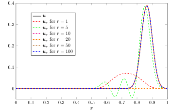
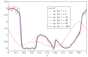
Figure 1: Test case 1: comparison for discontinuous (left) and continuous (right) initial conditions at final times of the exact solution 𝒖𝒖\boldsymbol{u} and the approximation 𝒖rsubscript𝒖𝑟\boldsymbol{u}_{r} computed with MTI for r{1,5,10,20,50,100}𝑟15102050100r\in\{1,5,10,20,50,100\}.
Relative errors for ucont0superscriptsubscript𝑢𝑐𝑜𝑛𝑡0u_{cont}^{0}
dim(Xr)dimensionsubscript𝑋𝑟\dim(X_{r}) E2subscript𝐸2E_{2} Esubscript𝐸E_{\infty}
111 0.0278310.0278310.027831 0.760580.760580.76058
222 0.0240750.0240750.024075 0.957130.957130.95713
555 0.00784610.00784610.0078461 0.269840.269840.26984
101010 0.000218530.000218530.00021853 0.00751560.00751560.0075156
202020 4.8616e094.8616𝑒094.8616e-09 1.6719e071.6719𝑒071.6719e-07
505050 4.0924e174.0924𝑒174.0924e-17 1.4074e151.4074𝑒151.4074e-15
100100100 4.4353e174.4353𝑒174.4353e-17 1.5253e151.5253𝑒151.5253e-15
200200200 4.5623e174.5623𝑒174.5623e-17 1.569e151.569𝑒151.569e-15
Relative errors for udisc0superscriptsubscript𝑢𝑑𝑖𝑠𝑐0u_{disc}^{0}
dim(Xr)dimensionsubscript𝑋𝑟\dim(X_{r}) E2subscript𝐸2E_{2} Esubscript𝐸E_{\infty}
111 0.0221160.0221160.022116 0.760580.760580.76058
222 0.01350.01350.0135 0.464270.464270.46427
555 0.00604240.00604240.0060424 0.20780.20780.2078
101010 0.00400440.00400440.0040044 0.137710.137710.13771
202020 0.0020430.0020430.002043 0.070260.070260.07026
505050 4.7139e054.7139𝑒054.7139e-05 0.00162110.00162110.0016211
100100100 1.3891e121.3891𝑒121.3891e-12 4.7771e114.7771𝑒114.7771e-11
200200200 6.3966e176.3966𝑒176.3966e-17 2.1998e152.1998𝑒152.1998e-15
Table 1: Test case 1: relative errors E2subscript𝐸2E_{2} and Esubscript𝐸E_{\infty} obtained with the MTI with respect to dim(Xr)dimensionsubscript𝑋𝑟\dim(X_{r}) for both continuous (left) and discontinuous (right) initial conditions conditions.

As shown onFigure 1, the approximations obtained with MTI are satisfactory when the dimension of the reduced space Xrsubscript𝑋𝑟X_{r} is greater than 202020. This is confirmed by the values of the relative errors Eq=𝒖r𝒖I,q/𝒖I,qsubscript𝐸𝑞subscriptnormsubscript𝒖𝑟𝒖𝐼𝑞subscriptnorm𝒖𝐼𝑞E_{q}=\|\boldsymbol{u}_{r}-\boldsymbol{u}\|_{I,q}/\|\boldsymbol{u}\|_{I,q} given in Table 1 for q=2𝑞2q=2 and q=𝑞q=\infty, where 𝒖I,qsubscriptnorm𝒖𝐼𝑞\|\boldsymbol{u}\|_{I,q} is the natural norm on Lq(I;X)superscript𝐿𝑞𝐼𝑋L^{q}(I;X). In particular, the relative error in L2superscript𝐿2L^{2}-norm (resp Lsuperscript𝐿L^{\infty}-norm) is of order 1017superscript101710^{-17} (respectively 1015superscript101510^{-15}) for a space Xrsubscript𝑋𝑟X_{r} with a reduced dimension of 505050. As expected, MTD, with a reduced space X1(t)subscript𝑋1𝑡X_{1}(t) of dimension 1 containing the exact solution, gives relative errors at the machine precision (E2=5.7 1017subscript𝐸2superscript5.71017E_{2}=5.7\,10^{-17} and E=1.3 1015subscript𝐸superscript1.31015E_{\infty}=1.3\,10^{-15}) For obtaining a very accurate precision, the method MTI requires a reduced space with rather high dimension, thus highlighting the limits of the POD method for transport equations. Now, we illustrate the impact of the smoothness of the solution. For this purpose, we consider the same test case with a discontinuous initial condition given by udisc0(x)=𝟏[0.1,0.9](x)(3x+sin(10x))superscriptsubscript𝑢𝑑𝑖𝑠𝑐0𝑥subscript10.10.9𝑥3𝑥10𝑥u_{disc}^{0}(x)=\boldsymbol{1}_{[0.1,0.9]}(x)\cdot(\lfloor 3x\rfloor+\sin(10x)) 222 Here, 𝟏Asubscript1𝐴\boldsymbol{1}_{A} is the characteristic function of a subset Ad𝐴superscript𝑑A\subset\mathbb{R}^{d} and x𝑥\lfloor x\rfloor denotes the integer part of x𝑥x.. The approximate solution is plotted onFigure 1 and the relative errors between the reduced approximation and the exact solution are summarized in the right table of Table 1. Here, we clearly observe that for non smooth initial condition udisc0superscriptsubscript𝑢𝑑𝑖𝑠𝑐0u_{disc}^{0} a reduced space with higher dimension is needed for well approximating the solution (e.g. dimension 200 against 50 for reaching the machine precision). Concerning the MTD, we still obtain relative errors up to the machine precision with a one-dimensional time dependent reduced space (E2=3.9 1017subscript𝐸2superscript3.91017E_{2}=3.9\,10^{-17} and E=1.3 1015subscript𝐸superscript1.31015E_{\infty}=1.3\,10^{-15}).

General case

We now consider the parameter-dependent problem and compare the approximations obtained with MTI and MTD for a subspace of dimension r=20𝑟20r=20 generated from a training set of size 303030. Figure 2 plots the evolution with time of the approximation obtained with MTD evaluated at 𝝃=0.65𝝃0.65\boldsymbol{\xi}=0.65. In Figure 3, the exact solution is compared to the approximations obtained by MTI and MTD, at final time and for 𝝃=0.65𝝃0.65\boldsymbol{\xi}=0.65. The solutions of the reduced order models are very close to the exact solution. Nevertheless, we notice that the approximation computed with MTI present small oscillations whereas the one obtained with MTD matches very well the exact solution (see right plot ofFigure 3).
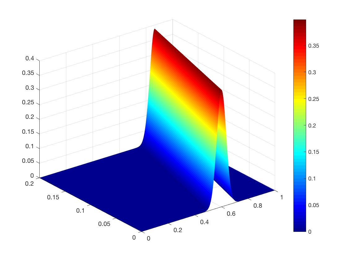
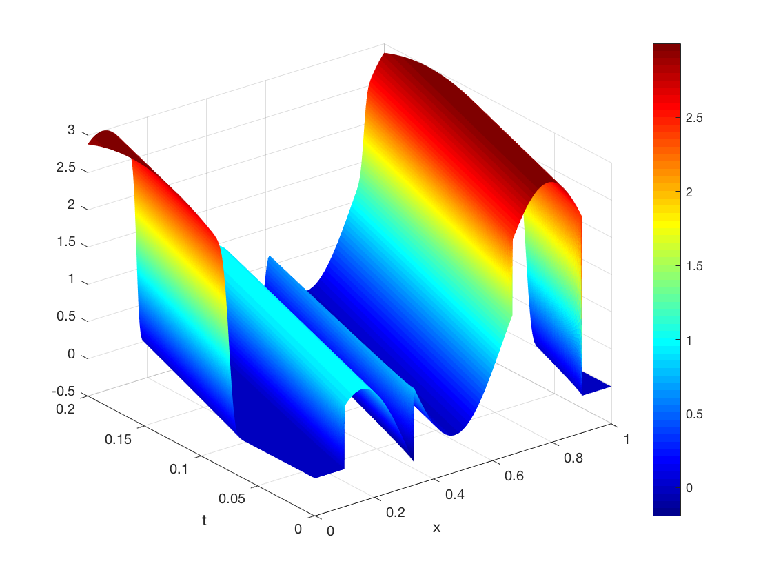
Refer to caption
Refer to caption
Figure 2: Test case 1: Time evolution of 𝒖rsubscript𝒖𝑟\boldsymbol{u}_{r} computed with MTD for r=20𝑟20r=20 and 𝝃=0.65𝝃0.65\boldsymbol{\xi}=0.65.
Refer to caption
Refer to caption
Figure 3: Test case 1: Reduced approximations 𝒖rsubscript𝒖𝑟\boldsymbol{u}_{r} provided by MTD and MTI compared to the exact solution 𝒖𝒖\boldsymbol{u} for both continuous (left) and discontinuous (right) initial conditions, at final time T=1𝑇1T=1 for r=20𝑟20r=20 and 𝝃=0.65𝝃0.65\boldsymbol{\xi}=0.65.

Then, we estimate the expectation 𝔼(Eq(𝝃))𝔼subscript𝐸𝑞𝝃\mathbb{E}(E_{q}(\boldsymbol{\xi})) and maximum max𝝃𝚵(Eq(𝝃))subscript𝝃𝚵subscript𝐸𝑞𝝃\max_{\boldsymbol{\xi}\in\boldsymbol{\Xi}}(E_{q}(\boldsymbol{\xi})) of the relative errors Eqsubscript𝐸𝑞E_{q} respectively by the empirical mean and by the maximum of the values of Eqsubscript𝐸𝑞E_{q} taken at 505050 randomly chosen values of the parameters. These quantities are depicted onFigure 4 for different values of r𝑟r and for both continuous and discontinuous initial conditions. For the same dimension of the reduced spaces, MTD clearly provides a more accurate approximation than MTI in particular when considering discontinuous initial condition.

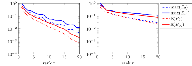
Refer to caption
Refer to caption
Figure 4: Test case 1: Statistical estimations of the expectation and maximum of the relative errors E2subscript𝐸2E_{2} and Esubscript𝐸E_{\infty} with respect to the reduced dimension r𝑟r, for MTD (left) and MTI (right) for both continuous (top) and discontinuous (bottom) initial conditions.
Validation of the error estimate

We now investigate the efficiency of the proposed error estimate Δ~rsubscript~Δ𝑟\tilde{\Delta}_{r}.Figure 5 shows the evolution with time of Δ~r(t,𝝃)subscript~Δ𝑟𝑡𝝃\tilde{\Delta}_{r}(t,\boldsymbol{\xi}) and the exact error 𝒆rXsubscriptnormsubscript𝒆𝑟𝑋\|\boldsymbol{e}_{r}\|_{X} for MTD and MTI, evaluated at 𝝃=0.65𝝃0.65\boldsymbol{\xi}=0.65. As expected, we observe that the error estimates have an exponential behavior in time. The error estimate Δ~rsubscript~Δ𝑟\tilde{\Delta}_{r} is much sharper for MTD than for MTI. For MTI, Δ~rsubscript~Δ𝑟\tilde{\Delta}_{r} is a very pessimistic upper bound of the error. This observation is confirmed by computing the effectivity index κ(t,𝝃)=Δ~r(t,𝝃)/𝒆r(t,𝝃)X𝜅𝑡𝝃subscript~Δ𝑟𝑡𝝃subscriptnormsubscript𝒆𝑟𝑡𝝃𝑋\kappa(t,\boldsymbol{\xi})=\tilde{\Delta}_{r}(t,\boldsymbol{\xi})/\|\boldsymbol{e}_{r}(t,\boldsymbol{\xi})\|_{X}. Figure 11 plots the evolution with time of a statistical estimation of the mean of the effectivity index 𝔼(κ(t,𝝃))𝔼𝜅𝑡𝝃\mathbb{E}(\kappa(t,\boldsymbol{\xi})), which remains close to 111 with MTD and takes high values with MTI.

Refer to caption
Refer to caption
Figure 5: Test case 1: Evolution with time of Δ~r(t,𝝃)subscript~Δ𝑟𝑡𝝃\tilde{\Delta}_{r}(t,\boldsymbol{\xi}) and 𝒆r(t,𝝃)Xsubscriptnormsubscript𝒆𝑟𝑡𝝃𝑋\|\boldsymbol{e}_{r}(t,\boldsymbol{\xi})\|_{X} for MTD (left) and MTI (right) for both continuous (top) and discontinuous (bottom) initial conditions, for r=20𝑟20r=20 and 𝝃=0.65𝝃0.65\boldsymbol{\xi}=0.65.
Refer to caption
Figure 6: Test case 1: Evolution with time of a statistical estimation of 𝔼(κ(t,𝝃))𝔼𝜅𝑡𝝃\mathbb{E}(\kappa(t,\boldsymbol{\xi})) for MTD (left) and MTI (right) for both continuous and discontinuous initial conditions.
CPU times

Now, we briefly discuss the CPU computational costs of both MTI and MTD methods with POD-greedy and T-greedy algorithms respectively. We restrict the presentation to the case of the initial condition udisc0subscriptsuperscript𝑢0𝑑𝑖𝑠𝑐u^{0}_{disc} (similar results are observed for ucont0subscriptsuperscript𝑢0𝑐𝑜𝑛𝑡u^{0}_{cont}). The dimension of reduced spaces is fixed to r=20𝑟20r=20 for both methods. As summarized in Table 2, both offline and online costs are roughly of the same order but the MTD provides a reduced order model which is by 222 orders of magnitude (see Figure 4) better than the reduced order model provided by MTI. Yet, we notice that for the MTI, CPU-times are slightly higher. This is probably due to additional computations involved by time-dependent reduced quantities in MTD. We may guess that the CPU times for both methods would be similar for non autonomous problems with time affine dependent coefficients.

Offline Online
MTD 1955.11955.11955.1 11.2411.2411.24
MTI 1517.51517.51517.5 8.948.948.94
Table 2: Test case 1: Offline and online CPU-times for both MTD and MTI, with udisc0superscriptsubscript𝑢𝑑𝑖𝑠𝑐0u_{disc}^{0}.

5.2 Test case 2

We now consider a two-dimensional advection-diffusion equation with source term g=0𝑔0g=0, c(u,𝝃)=0𝑐𝑢𝝃0c(u,\boldsymbol{\xi})=0, μ(𝝃)=μ0(2+cos(πξ1)2)\mu(\boldsymbol{\xi})=\mu^{0}(2+\cos(\pi\xi^{1})^{2}), with μ0=0.5superscript𝜇00.5\mu^{0}=0.5, and a(𝒙,𝝃)=a(𝝃)(x20.5,0.5x1)T𝑎𝒙𝝃𝑎𝝃superscriptsubscript𝑥20.50.5subscript𝑥1𝑇a(\boldsymbol{x},\boldsymbol{\xi})=a(\boldsymbol{\xi})(x_{2}-0.5,0.5-x_{1})^{T}, with a(𝝃)=a0sin(πξ2)𝑎𝝃subscript𝑎0𝜋superscript𝜉2a(\boldsymbol{\xi})=a_{0}\sin(\pi\xi^{2}) and a0=0.1subscript𝑎00.1a_{0}=0.1. Here, we choose ξ1,ξ2U(1,1)similar-tosuperscript𝜉1superscript𝜉2𝑈11\xi^{1},\xi^{2}\sim U(-1,1) as independent uniform random variables. The spatial domain is Ω=(0,1)2Ωsuperscript012\Omega=(0,1)^{2} and the time interval I=(0,0.2)𝐼00.2I=(0,0.2). The initial condition is given by u0(x)=e(x123)2(x223)2sin(2πx1)sin(2πx2)superscript𝑢0𝑥superscript𝑒superscriptsubscript𝑥1232superscriptsubscript𝑥22322𝜋subscript𝑥12𝜋subscript𝑥2u^{0}(x)=e^{-(x_{1}-\frac{2}{3})^{2}-(x_{2}-\frac{2}{3})^{2}}\sin(2\pi x_{1})\sin(2\pi x_{2}) and we impose homogeneous Dirichlet boundary conditions. We consider a 1subscript1\mathbb{P}_{1}-Lagrange finite element discretization with n=1681𝑛1681n=1681 nodes 333The mesh is chosen fine enough to ensure a Péclet number smaller than 1. together with an implicit Euler scheme with K=400𝐾400K=400 time steps, yielding the following scheme

(𝐈Xδt𝐀(𝝃))𝒖k+1(𝝃)=𝒖k(𝝃),subscript𝐈𝑋𝛿𝑡𝐀𝝃superscript𝒖𝑘1𝝃superscript𝒖𝑘𝝃(\mathbf{I}_{X}-\delta t\mathbf{A}(\boldsymbol{\xi}))\boldsymbol{u}^{k+1}(\boldsymbol{\xi})=\boldsymbol{u}^{k}(\boldsymbol{\xi}), (29)

with 𝐀(𝝃)=μ(𝝃)𝐀D+a(𝝃)𝐀Cd×d𝐀𝝃𝜇𝝃subscript𝐀𝐷𝑎𝝃subscript𝐀𝐶superscript𝑑𝑑\mathbf{A}(\boldsymbol{\xi})=\mu(\boldsymbol{\xi})\mathbf{A}_{D}+a(\boldsymbol{\xi})\mathbf{A}_{C}\in\mathbb{R}^{d\times d} (d=1521𝑑1521d=1521), where 𝐀Csubscript𝐀𝐶\mathbf{A}_{C} and 𝐀Dsubscript𝐀𝐷\mathbf{A}_{D} are the product of the mass matrix inverse with the discrete two dimensional diffusion and convection operators, obtained by finite element approximation, respectively.

We first present the reduced approximations computed by MTI and MTD with reduced spaces of dimension r=30𝑟30r=30 selected with greedy algorithms using a training set of size 606060. Figure 7 represents the approximation obtained with MTD evaluated for different values of the parameter 𝝃{(0.2,1),(0.2,0),(0.2,0.5)}𝝃0.210.200.20.5\boldsymbol{\xi}\in\{(0.2,-1),(0.2,0),(0.2,0.5)\}.

Refer to caption
Refer to caption
Refer to caption
Figure 7: Test case 2: reduced approximation 𝒖rsubscript𝒖𝑟\boldsymbol{u}_{r} computed with MTD for r=30𝑟30r=30 at final time and 𝝃{(0.2,1),(0.2,0),(0.2,0.5)}𝝃0.210.200.20.5\boldsymbol{\xi}\in\{(0.2,-1),(0.2,0),(0.2,0.5)\}.

For the same parameter values, the absolute distance to the exact solution at final time is given onFigure 7 for MTI and MTD. It shows that the approximations obtained by both order reduction methods are in good agreement with the exact solution. Once again, we observe that MTD provides a better approximation with an error of order 109superscript10910^{-9} against 105superscript10510^{-5} for MTI.

Refer to caption
Refer to caption
Refer to caption
Refer to caption
Refer to caption
Refer to caption
Figure 8: Test case 2: absolute error between the exact solution and reduced approximations |𝒖𝒖r|𝒖subscript𝒖𝑟|\boldsymbol{u}-\boldsymbol{u}_{r}| provided by MTD (top) and MTI (bottom) at final time for r=30𝑟30r=30 and 𝝃{(0.2,1),(0.2,0),(0.2,0.5)}𝝃0.210.200.20.5\boldsymbol{\xi}\in\{(0.2,-1),(0.2,0),(0.2,0.5)\}.

Estimations of the expectations 𝔼(Eq(𝝃))𝔼subscript𝐸𝑞𝝃\mathbb{E}(E_{q}(\boldsymbol{\xi})) and maxima max𝝃𝚵(Eq(𝝃))subscript𝝃𝚵subscript𝐸𝑞𝝃\max_{\boldsymbol{\xi}\in\boldsymbol{\Xi}}(E_{q}(\boldsymbol{\xi})) of the relative errors Eqsubscript𝐸𝑞E_{q} (using a random sample of size 505050 in 𝚵𝚵\boldsymbol{\Xi}) are plotted on Figure 9 for different values of r𝑟r. For this advection-diffusion problem, we first observe that both order reduction methods provide accurate approximations with low-dimensional spaces. However, for the same dimension of the reduced spaces, the approximation obtained by MTD is more accurate than the approximation obtained by MTI. Indeed, in order to reach a relative error of 108superscript10810^{-8}, MTD requires r=10𝑟10r=10 while MTI requires r=30𝑟30r=30.

Refer to caption
Figure 9: Test case 2: Statistical estimations of the expectation and maximum of the relative errors E2subscript𝐸2E_{2} and Esubscript𝐸E_{\infty} with respect to the reduced dimension r𝑟r, for MTD (left) and MTI (right).
Error estimates

Figure 10 represents the evolution with time of the exact error 𝒆r(t,𝝃)Xsubscriptnormsubscript𝒆𝑟𝑡𝝃𝑋\|\boldsymbol{e}_{r}(t,\boldsymbol{\xi})\|_{X} and of the error estimate Δ~r(t,𝝃)subscript~Δ𝑟𝑡𝝃\tilde{\Delta}_{r}(t,\boldsymbol{\xi}) for both order reduction methods, for 𝝃=(0.2,0.5)𝝃0.20.5\boldsymbol{\xi}=(0.2,0.5). Again, we observe the exponential behavior of the error estimates. The errors obtained by MTD are several orders of magnitude lower than the errors obtained by MTI.
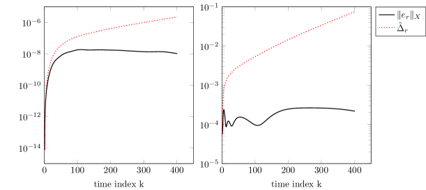
Refer to caption
Figure 10: Test case 2: Evolution with time of the error estimate Δ~rsubscript~Δ𝑟\tilde{\Delta}_{r} and true error 𝒆rXsubscriptnormsubscript𝒆𝑟𝑋\|\boldsymbol{e}_{r}\|_{X} for MTD (left) and MTI (right), for r=30𝑟30r=30 and 𝝃=(0.2,0.5)𝝃0.20.5\boldsymbol{\xi}=(0.2,0.5).

For the first time indices (i.e. k<100𝑘100k<100), Δ~rsubscript~Δ𝑟\tilde{\Delta}_{r} provides a sharper error bound for MTD than for MTI. Also, Δ~rsubscript~Δ𝑟\tilde{\Delta}_{r} and the true error have quite similar time evolutions for MTD, and very different time evolutions for MTI. The superiority of MTD over MTI is confirmed onFigure 11, where we observe that the expectations of the effectivity index κ(t,𝝃)𝜅𝑡𝝃\kappa(t,\boldsymbol{\xi}) of MTI and MTD are in a ratio of 10. For longer times, the error estimates present similar efficiency for both approaches.
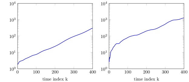
Refer to caption
Figure 11: Test case 2: Evolution with time of a statistical estimation of the expected effectivity index 𝔼(κ(t,𝝃))𝔼𝜅𝑡𝝃\mathbb{E}(\kappa(t,\boldsymbol{\xi})) for MTD (left) and MTI (right).
Study of greedy algorithms

Now, we study the behavior of the T-greedy and POD-greedy algorithms used for the construction of reduced spaces for MTD and MTI respectively. For both algorithms, the evolution with the iteration r𝑟r of the maximum of Δr(0,T)(𝝃)superscriptsubscriptΔ𝑟0𝑇𝝃\Delta_{r}^{(0,T)}(\boldsymbol{\xi}) over the training set 𝚵trainsubscript𝚵𝑡𝑟𝑎𝑖𝑛\boldsymbol{\Xi}_{train} is plotted onFigure 12. Note that at iteration r𝑟r, the dimension of the reduced space is actually r+1𝑟1r+1. We observe that the error decreases faster with r𝑟r for the T-greedy algorithm than for the POD-greedy algorithm. For example, at iteration 202020 of the greedy algorithms, the errors for POD-greedy and T-greedy algorithms are respectively of order 101superscript10110^{-1} and 101010. When stopping the greedy algorithms at a given precision, the dimension of the obtained reduced space is much smaller for T-greedy than for POD-greedy. We observe on Table 13 that the POD-greedy algorithm can select several times the same point in 𝚵𝚵\boldsymbol{\Xi} (for example, the value 𝝃=(0.3192,0.9004)𝝃0.31920.9004\boldsymbol{\xi}=(-0.3192,0.9004) is selected 6 times during the 303030 iterations). This is due to the fact that at each iteration, only the first term of the POD of the selected trajectory is added to the reduced space (here =11\ell=1). Concerning the T-greedy approach, a point in 𝚵𝚵\boldsymbol{\Xi} can be selected only once. This implies that for a fixed dimension, the POD-greedy approach requires less solutions of the full order dynamical system (here 555 for POD-greedy against 303030 for the T-greedy approach when considering a reduced space of dimension 303030). To illustrate this point, the number of calls to the full order problem with respect to maxξ𝚵trainΔr(0,T)(𝝃)subscript𝜉subscript𝚵𝑡𝑟𝑎𝑖𝑛superscriptsubscriptΔ𝑟0𝑇𝝃\max_{\xi\in\boldsymbol{\Xi}_{train}}\Delta_{r}^{(0,T)}(\boldsymbol{\xi}) is represented on the right curve ofFigure 12. The number of calls to the full order problem for POD-greedy algorithm remains smaller, which means that the POD-greedy algorithm uses only the information of snapshots already computed to enrich Xrsubscript𝑋𝑟X_{r} whereas the T-greedy algorithm requires new snapshots at each iteration. In terms of computational costs, the POD-greedy stategy presents lower offline computational costs since it requires a smaller number of calls to the full order problem, but for a given precision, it leads to larger reduced systems in the online step. For the T-greedy algorithm, we have the opposite conclusions. For a given precision, it leads to lower dimensional reduced spaces, and therefore to lower online costs, but it requires more calls to the full-order problem in the offline step. The MTD approach with POD-greedy remains a good alternative when treating autonomous linear dynamical systems arising from the discretization of linear parabolic problems with time independent matrices. Furthermore, contrarily to MTI, it does not require to store sequences of time dependent reduced quantities. But when considering non-autonomous dynamical systems (which requires handling time-dependent reduced quantities), the storing costs will be smaller with MTD, since this latter approach provides smaller reduced spaces for a given precision.
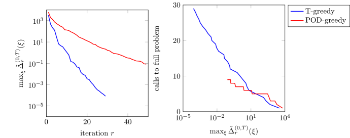
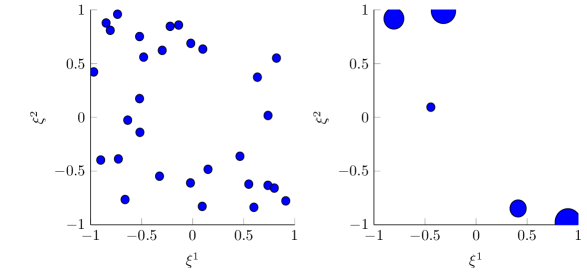
Refer to caption
Figure 12: Test case 2 : Evolution of the maximum of Δ~r(0,T)(𝝃)superscriptsubscript~Δ𝑟0𝑇𝝃\tilde{\Delta}_{r}^{(0,T)}(\boldsymbol{\xi}) over 𝚵trainsubscript𝚵𝑡𝑟𝑎𝑖𝑛\boldsymbol{\Xi}_{train} with the iteration r𝑟r (left), and number of calls to the full order problem with respect to the maximum of Δ~r(0,T)(𝝃)superscriptsubscript~Δ𝑟0𝑇𝝃\tilde{\Delta}_{r}^{(0,T)}(\boldsymbol{\xi}) over 𝚵trainsubscript𝚵𝑡𝑟𝑎𝑖𝑛\boldsymbol{\Xi}_{train} (right), for T-greedy (blue line) and POD-greedy (red line) algorithms.
Refer to caption
Figure 13: Test case 2: Selected points in 𝚵𝚵\boldsymbol{\Xi} for the T-greedy (left) and POD-greedy (right) algorithms during 303030 iterations. For POD-greedy, the size of a point increases with the number of times it is selected.
CPU times

As shown in Table 3, CPU-times for both offline and online phases are again similar, when the reduced space dimension is fixed to r=30𝑟30r=30 for both MTI and MTD. We still observe a small additional cost for the online phase of MTD due to computations with time-dependent reduced quantities, but MTD again provides a better reduced approximation (see Figure 9). Concerning the POD-greedy algorithm, one could imagine to improve the offline cost by storing the solution trajectories computed during the greedy procedure for parameters selected several times, but this would imply additional storage costs.

Offline - Basis selection Offline - Reduced quantities Online
T-Greedy 349073490734907 77.6977.6977.69 37.8637.8637.86
POD-Greedy 327673276732767 0.220.220.22 34.634.634.6
Table 3: Test case 2: Offline and online CPU-times for both MTD and MTI.

5.3 Test case 3

We study a nonlinear viscous Burger’s equation with uncertain parameters. This test case is adapted from [34]. We consider a spatial domain Ω=(0,1)Ω01\Omega=(0,1), a time interval I=(0,1)𝐼01I=(0,1), homogeneous Dirichlet boundary conditions and an initial condition u0=0superscript𝑢00u^{0}=0. We consider c(u,𝝃)=12u𝑐𝑢𝝃12𝑢c(u,\boldsymbol{\xi})=\frac{1}{2}u, a(x,𝝃)=0𝑎𝑥𝝃0a(x,\boldsymbol{\xi})=0 and a diffusion coefficient μ(𝝃)=ξ𝜇𝝃𝜉\mu(\boldsymbol{\xi})=\xi, with ξU(0.01,0.06)similar-to𝜉𝑈0.010.06\xi\sim U(0.01,0.06) a uniform random variable. The source term is defined by g(x,t,𝝃)=g1(x,t)+g2(x,t)𝑔𝑥𝑡𝝃subscript𝑔1𝑥𝑡subscript𝑔2𝑥𝑡g(x,t,\boldsymbol{\xi})=g_{1}(x,t)+g_{2}(x,t), with

g1(x,t)=4e(x0.20.03)2𝟏[0.1,0.3](x)sin(4πt),subscript𝑔1𝑥𝑡4superscript𝑒superscript𝑥0.20.032subscript10.10.3𝑥4𝜋𝑡\displaystyle g_{1}(x,t)=4e^{-(\frac{x-0.2}{0.03})^{2}}\boldsymbol{1}_{[0.1,0.3]}(x)\sin(4\pi t),
g2(x,t)=4𝟏[0.6,0.7](x)𝟏[0.2,0.4](t).subscript𝑔2𝑥𝑡4subscript10.60.7𝑥subscript10.20.4𝑡\displaystyle g_{2}(x,t)=4\cdot\boldsymbol{1}_{[0.6,0.7]}(x)\boldsymbol{1}_{[0.2,0.4]}(t).

The term g1subscript𝑔1g_{1} corresponds to an excitation localized in space and oscillating with time, whereas the term g2subscript𝑔2g_{2} corresponds to a constant excitation over a localized space-time region. We use a finite difference scheme in space (with n=300𝑛300n=300 nodes, and d=298𝑑298d=298) with uniform mesh (as in Subsection 5.1) and a semi-implicit Euler scheme in time (with K=200𝐾200K=200 time steps), yielding the following scheme:

(𝐈Xδt𝐀(𝝃))𝒖k+1(𝝃)=𝒖k(𝝃)+δt(𝒉(𝒖k)+𝒈k),subscript𝐈𝑋𝛿𝑡𝐀𝝃superscript𝒖𝑘1𝝃superscript𝒖𝑘𝝃𝛿𝑡𝒉superscript𝒖𝑘superscript𝒈𝑘(\mathbf{I}_{X}-\delta t\mathbf{A}(\boldsymbol{\xi}))\boldsymbol{u}^{k+1}(\boldsymbol{\xi})=\boldsymbol{u}^{k}(\boldsymbol{\xi})+\delta t(\boldsymbol{h}(\boldsymbol{u}^{k})+\boldsymbol{g}^{k}), (30)

where 𝐀d×d𝐀superscript𝑑𝑑\mathbf{A}\in\mathbb{R}^{d\times d} denotes the discrete second derivative operator, and where the discrete flux 𝒉(𝒖k)d𝒉superscript𝒖𝑘superscript𝑑\boldsymbol{h}(\boldsymbol{u}^{k})\in\mathbb{R}^{d} is defined by (𝒉(𝒖k))i=uik(𝐂𝒖k)isubscript𝒉superscript𝒖𝑘𝑖superscriptsubscript𝑢𝑖𝑘subscript𝐂superscript𝒖𝑘𝑖(\boldsymbol{h}(\boldsymbol{u}^{k}))_{i}=-u_{i}^{k}(\mathbf{C}\boldsymbol{u}^{k})_{i} with 𝐂d×d𝐂superscript𝑑𝑑\mathbf{C}\in\mathbb{R}^{d\times d} the matrix associated with the discrete first derivative operator.

Reduced spaces are constructed with POD-greedy and T-greedy algorithms with a training set of size 606060. For the error estimation, we have used a nearest neighbor interpolation of the Lipschitz constant of the flux 𝒉𝒉\boldsymbol{h}. The maximum ML(𝝃)subscript𝑀𝐿𝝃M_{L}(\boldsymbol{\xi}) and minimum mL(𝝃)subscript𝑚𝐿𝝃m_{L}(\boldsymbol{\xi}) of L~X[𝒉](𝒖r(t,𝝃),t,𝝃)LX[𝒉](𝒖r(t,𝝃),t,𝝃)subscript~𝐿𝑋delimited-[]𝒉subscript𝒖𝑟𝑡𝝃𝑡𝝃subscript𝐿𝑋delimited-[]𝒉subscript𝒖𝑟𝑡𝝃𝑡𝝃\frac{\tilde{L}_{X}[\boldsymbol{h}](\boldsymbol{u}_{r}(t,\boldsymbol{\xi}),t,\boldsymbol{\xi})}{L_{X}[\boldsymbol{h}](\boldsymbol{u}_{r}(t,\boldsymbol{\xi}),t,\boldsymbol{\xi})} over the time interval I𝐼I have been computed for both MTD and MTI methods (see Table 4). We observe that the values are localized in intervals whose bounds are close to 111, which indicates that the approximations are quite satisfactory. For the efficient evaluation of the nonlinear flux 𝒉𝒉\boldsymbol{h}, an EIM has been used with a tolerance ε=1010𝜀superscript1010\varepsilon=10^{-10} in the stopping criterion (24). For the considered simulations, it corresponds to an average number m𝑚m of terms in the EIM equal to 103103103 and 108108108 for MTD and MTI respectively. As shown in Table 4, the maximum of the relative errors E𝒉(t,𝝃)=𝒉(ur(t,𝝃),t,𝝃)𝒉~(ur(t,𝝃),t,𝝃)X/𝒉(ur(t,𝝃),t,𝝃)Xsubscript𝐸𝒉𝑡𝝃subscriptnorm𝒉subscript𝑢𝑟𝑡𝝃𝑡𝝃~𝒉subscript𝑢𝑟𝑡𝝃𝑡𝝃𝑋subscriptnorm𝒉subscript𝑢𝑟𝑡𝝃𝑡𝝃𝑋E_{\boldsymbol{h}}(t,\boldsymbol{\xi})=\|\boldsymbol{h}(u_{r}(t,\boldsymbol{\xi}),t,\boldsymbol{\xi})-\tilde{\boldsymbol{h}}(u_{r}(t,\boldsymbol{\xi}),t,\boldsymbol{\xi})\|_{X}/\|\boldsymbol{h}(u_{r}(t,\boldsymbol{\xi}),t,\boldsymbol{\xi})\|_{X} on the flux is of order 1010superscript101010^{-10} as expected.

maxtE𝒉(𝝃,t)subscript𝑡subscript𝐸𝒉𝝃𝑡\max_{t}E_{\boldsymbol{h}}(\boldsymbol{\xi},t) [mL(𝝃),ML(𝝃)]subscript𝑚𝐿𝝃subscript𝑀𝐿𝝃[m_{L}(\boldsymbol{\xi}),M_{L}(\boldsymbol{\xi})]
𝝃𝝃\boldsymbol{\xi} MTI MTD MTI MTD
0.010.010.01 1.555010101.5550superscript10101.5550~{}10^{-10} 4.220810104.2208superscript10104.2208~{}10^{-10} [0.9116,1.1011]0.91161.1011[0.9116,1.1011] [1.1055,1.1297]1.10551.1297[1.1055,1.1297]
0.0350.0350.035 3.580310103.5803superscript10103.5803~{}10^{-10} 1.440010111.4400superscript10111.4400~{}10^{-11} [0.7804,0.9536]0.78040.9536[0.7804,0.9536] [1.0062,1.0483]1.00621.0483[1.0062,1.0483]
0.060.060.06 5.037410105.0374superscript10105.0374~{}10^{-10} 1.420110111.4201superscript10111.4201~{}10^{-11} [0.7567,1.0009]0.75671.0009[0.7567,1.0009] [0.9947,0.9989]0.99470.9989[0.9947,0.9989]
Table 4: Test case 3 : Maximum over the time interval of the relative approximation error of the flux 𝒉𝒉\boldsymbol{h} with EIM, and minimum and maximum values mLsubscript𝑚𝐿m_{L} and MLsubscript𝑀𝐿M_{L} of the ratio between approximate and exact Lipschitz constants of 𝒉𝒉\boldsymbol{h}, for MTD and MTI.

We first study the behavior of the approximations provided by the MTD and MTI evaluated for the parameter values 𝝃{0.01,0.035,0.06}𝝃0.010.0350.06\boldsymbol{\xi}\in\{0.01,0.035,0.06\} and for r=15𝑟15r=15. The evolution of the solution of the reduced order model obtained with MTD is plotted on Figure 14. We clearly observe different features for different values of the diffusion coefficient.Figure 15 represents the exact solution and the approximations obtained by MTD and MTI at final time and for a given value of the parameter. For r=15𝑟15r=15, the reduced approximations are in good agreement with the exact solution. Nevertheless, we note that the approximation obtained with MTD is clearly better than with MTI.

ξ=0.01𝜉0.01\xi=0.01                            ξ=0.035𝜉0.035\xi=0.035                        ξ=0.06𝜉0.06\xi=0.06
Refer to caption

Figure 14: Test case 3 : Evolution over the space-time grid of the approximation 𝒖rsubscript𝒖𝑟\boldsymbol{u}_{r} computed with MTD for r=15𝑟15r=15 and for 𝝃{0.01,0.035,0.06}𝝃0.010.0350.06\boldsymbol{\xi}\in\{0.01,0.035,0.06\}.
Refer to caption
Figure 15: Test case 3 : Comparison between the exact solution 𝒖𝒖\boldsymbol{u} (black line) and the approximations 𝒖rsubscript𝒖𝑟\boldsymbol{u}_{r} obtained with MTD (blue dashed line) and MTI (red dotted line) with r=15𝑟15r=15, at final time T=0.1𝑇0.1T=0.1 and for 𝝃{0.01,0.035,0.06}𝝃0.010.0350.06\boldsymbol{\xi}\in\{0.01,0.035,0.06\}.

This superiority of MTD over MTI is confirmed byFigure 16 where we have plotted statistical estimations (with a random sample of size 505050) of the expectation and maximum of the relative errors. As we can see, MTD provides with r=15𝑟15r=15 an approximation with a relative error of 1010superscript101010^{-10}, whereas MTI only provides an approximation with a relative error of 102superscript10210^{-2} for the same dimension of the reduced space. For r=50𝑟50r=50, MTI provides an approximation with relative error 106superscript10610^{-6}, which is still higher than MTD with r=15𝑟15r=15.

Refer to caption
Figure 16: Test case 3: Statistical estimations of the expectations and maxima of the relative errors E2subscript𝐸2E_{2} and Esubscript𝐸E_{\infty} with respect to the reduced dimension r𝑟r, for MTD (left) and MTI (right).
Study of error estimates

We now compare the behavior of the error estimate Δ~rsubscript~Δ𝑟\tilde{\Delta}_{r} for MTD and MTI. Figure 17 represent the evolution with time of the exact error and of the error estimate for both methods, with and without approximation of the flux and the Lipchitz constants, for 𝝃=0.035𝝃0.035\boldsymbol{\xi}=0.035 and r=15𝑟15r=15. We first remark that the EIM approximation of the nonlinear flux as well as the approximated Lipschitz constants have a small impact on the behavior of the error estimate. Nevertheless we notice that for the first instants for MTD, where the error is smaller than 1010superscript101010^{-10}, the EIM error is no longer negligible and 𝒆rXsubscriptnormsubscript𝒆𝑟𝑋\|\boldsymbol{e}_{r}\|_{X} and Δ~rsubscript~Δ𝑟\tilde{\Delta}_{r} are slightly impacted. For MTD, a small difference is observed for final times only on Δ~rsubscript~Δ𝑟\tilde{\Delta}_{r}. This is probably due to the approximation of the Lipchitz constant. These differences disappear when choosing a smaller precision ε𝜀\varepsilon for MTD or when considering larger reduced spaces for MTI. Again, we obtain several orders of magnitude between the errors provided by the MTD and MTI. Here, the expectations of the effectivity index κ(t,𝝃)𝜅𝑡𝝃\kappa(t,\boldsymbol{\xi}) (plotted onFigure 18) are of the same order, with or without EIM, which means that the error estimate has the same efficiency for both approaches.
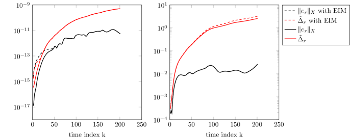
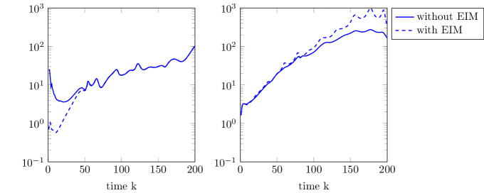
Refer to caption
Figure 17: Test case 3: Evolution with time of the error estimate Δ~rsubscript~Δ𝑟\tilde{\Delta}_{r} (dotted line) and the exact error 𝒆rXsubscriptnormsubscript𝒆𝑟𝑋\|\boldsymbol{e}_{r}\|_{X} (solid line), for MTD (left) and MTI (right), for 𝝃=0.035𝝃0.035\boldsymbol{\xi}=0.035 and r=15𝑟15r=15.
Refer to caption
Figure 18: Test case 3: Evolution with time of a statistical estimation of the expected effectivity index 𝔼(κ(t,𝝃))𝔼𝜅𝑡𝝃\mathbb{E}(\kappa(t,\boldsymbol{\xi})), for MTD (left) and MTI (right), for 𝝃=0.035𝝃0.035\boldsymbol{\xi}=0.035 and r=15𝑟15r=15.
Study of greedy algorithms

We finally study the behavior of the greedy algorithms used for the construction of the reduced space Xrsubscript𝑋𝑟X_{r}. Once again, we have plotted the evolution of the maximum of Δ~r(0,T)(𝝃)superscriptsubscript~Δ𝑟0𝑇𝝃\tilde{\Delta}_{r}^{(0,T)}(\boldsymbol{\xi}) over 𝚵trainsubscript𝚵𝑡𝑟𝑎𝑖𝑛\boldsymbol{\Xi}_{train} with the iteration r𝑟r and the number of calls to the full order problem with respect to the maximum of Δ~r(0,T)(𝝃)superscriptsubscript~Δ𝑟0𝑇𝝃\tilde{\Delta}_{r}^{(0,T)}(\boldsymbol{\xi}) onFigure 19. We observe the same behavior as for the test case 2. The maximum error during the greedy iterations decreases faster with T-greedy than with POD-greedy (T-greedy reaches a precision of order 106superscript10610^{-6} for the iteration 141414, while POD-greedy reaches a precision of 102superscript10210^{-2} for the iteration 494949). In terms of computational costs, the number of calls to the full order problem in the offline step is lower for T-greedy algorithm than for POD-greedy (e.g., for reaching a precision of order 102superscript10210^{-2}, T-greedy (resp. POD-greedy) algorithm requires 777 (resp. 11) calls to the full order problem). Contrary to the previous linear test case, the use of MTD with T-greedy algorithm clearly reduces the computational costs of both online and offline steps in comparison to a MTI combined with a POD-greedy construction of reduced spaces.
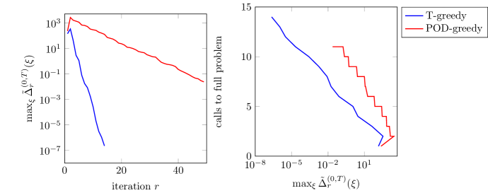
Refer to caption
Figure 19: Test case 3 : Evolution of the maximum of Δ~r(0,T)(𝝃)superscriptsubscript~Δ𝑟0𝑇𝝃\tilde{\Delta}_{r}^{(0,T)}(\boldsymbol{\xi}) over 𝚵trainsubscript𝚵𝑡𝑟𝑎𝑖𝑛\boldsymbol{\Xi}_{train} with the iteration r𝑟r (left), and number of calls to the full order problem with respect to the maximum of Δ~r(0,T)(𝝃)superscriptsubscript~Δ𝑟0𝑇𝝃\tilde{\Delta}_{r}^{(0,T)}(\boldsymbol{\xi}) over 𝚵trainsubscript𝚵𝑡𝑟𝑎𝑖𝑛\boldsymbol{\Xi}_{train} (right), for T-greedy (blue line) and POD-greedy (red line) algorithms.
CPU times

The dimension of reduced spaces is fixed to r=15𝑟15r=15 for both methods. As summarized in the table Table 5, once again for this problem, both offline and online cost are roughly of the same order for both MTI and MTD while MTD gives a finer reduced approximation which is by 8 orders of magnitude (see Figure 16) better than the one provided by MTI .

Offline (Basis) Offline (Reduction)
MTI 6137.26137.26137.2 9.229.229.22
MTD 6253.86253.86253.8 9.279.279.27
Table 5: Test case 1: Offline and online CPU-times for both MTD and MTI.

6 Conclusion

In this paper, we have presented a projection-based model order reduction approach for the solution of parameter-dependent dynamical systems. It relies on a Galerkin projection of the full order dynamical system on time-dependent reduced spaces. This generalizes classical model order reduction methods with time-independent reduced spaces. An a posteriori error estimate using the logarithmic Lipschitz constant associated to the flux has also been proposed and provides an efficient a posteriori error estimate. Using this error estimate, we have derived a greedy algorithm (called T-greedy algorithm) for the construction of a sequence of time-dependent reduced spaces. We have performed several numerical tests on both linear and nonlinear dynamical systems. The order reduction method with time-dependent spaces constructed with a T-greedy algorithm (MTD) has been compared to a method with time-independent spaces constructed with a POD-greedy algorithm (MTI). For the same online costs (time for evaluating the ROM), the error in the predictions of the ROM obtained by MTD may be several orders of magnitude lower than the error in the predictions of the ROM obtained by MTI. In other words, for a given precision of the ROM, the MTD approach yields a significant reduction of online computation costs. Here, the proposed T-greedy algorithm for the selection of parameters relies on an error indicator using a L2superscript𝐿2L^{2}-norm in time of an error estimate. This global error estimate could be improved by considering sharper local in time error estimates which could be obtained by improving the local Lipschitz constants used to derive our error bound [34]. Moreover, a goal-oriented variant of this algorithm could be introduced by considering norms taking into account a certain quantity of interest (e.g., the value of the solution at the final time) in order to improve the efficiency of the order reduction method for this approximation of this quantity of interest.

References

  • [1] M. Barrault, Y. Maday, N.C. Nguyen and A.T. Patera, An ”empirical interpolation” method: application to efficient reduced-basis discretization of partial differential equations. Comptes Rendus Mathématique, 339(9):667–672, 2004.
  • [2] U. Baur, P. Benner, B. Haasdonk, C. Himpe, I. Maiern and M.  Ohlberger, Comparison of methods for parametric model order reduction of instationary problems, preprint, 2015.
  • [3] M.  Bebendorf, Y. Maday and B. Stamm, Comparison of some Reduced Representation Approximations, Quarteroni, Alfio and Rozza, Gianluigi , Reduced Order Methods for Modeling and Computational Reduction, MS&A - Modeling, Simulation and Applications 9:67–100, 2014.
  • [4] P. Benner, S. Gugercin and K. Willcox, A Survey of Model Reduction Methods for Parametric Systems, preprint, 2013.
  • [5] P. Binev, A. Cohen, W. Dahmen, R. DeVore, G. Petrova and P. Wojtaszczyk, Convergence Rates for Greedy Algorithms in Reduced Basis Methods. SIAM Journal on Mathematical Analysis, 43(3):1457–1472, 2011.
  • [6] A.  Buffa, Y.  Maday, A.T. Patera, C. Prud’homme and G. Turinici, A priori convergence of the greedy algorithm for the parametrized reduced basis, ESAIM-Math. Model. Numer. Anal.,46(3):595–603,2012.
  • [7] T.T. Bui and K. Willcox and O. Ghattas, Model Reduction for Large-Scale Systems with High-Dimensional Parametric Input Space, SIAM Journal on Scientific Computing,6:3270–3288,2008.
  • [8] S. Chaturantabut and D.C. Sorensen, Nonlinear Model Reduction via Discrete Empirical Interpolation, SIAM Journal on Scientific Computing, 42(5):2737–2764, 2010.
  • [9] M. Cheng, T.Y. Hou and Z. Zhang and D.C. Sorensen, A dynamically bi-orthogonal method for time-dependent stochastic partial differential equations I: Derivation and algorithms, Journal of Computational Physics, 242(0):843-868, 2013.
  • [10] M. Cheng, T.Y. Hou and Z. Zhang and D.C. Sorensen, A dynamically bi-orthogonal method for time-dependent stochastic partial differential equations II: Adaptivity and generalizations , Journal of Computational Physics, 242(0):753 - 776,2013.
  • [11] R. DeVore, G. Petrova and P.  Wojtaszczyk Greedy algorithms for reduced bases in Banach spaces, Constructive Approximation, 37(3):455–466, 2013.
  • [12] M. Drohmann, B. Haasdonk and M. Ohlberger , Reduced Basis Approximation for Nonlinear Parametrized Evolution Equations based on Empirical Operator Interpolation , SIAM Journal on Scientific Computing, 34(2):A937–A969,2012.
  • [13] A posteriori error bounds for the empirical interpolation method, M NU ex A.M. Grepl and A.T. Patera, Comptes Rendus Mathématique, 348(9-10):575-579,2010.
  • [14] J.L. Eftang, D.J. Knezevic and A.T.  Patera , An hp certified reduced basis method for parametrized parabolic partial differential equations, Mathematical and Computer Modelling of Dynamical Systems, 17(4):395–422,2011.
  • [15] S. Glas, A. Mayerhofer, K. Urban, Two Ways to Treat Time in Reduced Basis Methods (preprint), 2016
  • [16] M.A.  Grepl and A.T. Patera, A posteriori error bounds for reduced-basis approximations of parametrized parabolic partial differential equations, ESAIM: Mathematical Modelling and Numerical Analysis, 39(01):157–181,2005.
  • [17] B.  Haasdonk M. Ohlberger, Reduced basis method for finite volume approximations of parametrized linear evolution equations, ESAIM: Mathematical Modelling and Numerical Analysis, 42(2);277–302, 2008.
  • [18] B.  Haasdonk M. Ohlberger, Efficient reduced models and a posteriori error estimation for parametrized dynamical systems by offline/online decomposition, Mathematical and Computer Modelling of Dynamical Systems, 17(2):145–161,2011
  • [19] B. Haasdonk , Convergence Rates of the POD-Greedy method , M2AN Math. Model. Numer. Anal., 47:859–873, 2015.
  • [20] B. Haasdonk, Reduced basis methods for parametrized PDEs - A tutorial introduction for stationary and instationary problems., Tech. Rep., 2014, Chapter to appear in P. Benner, A. Cohen, M. Ohlberger and K. Willcox : “Model reduction and approximation for complex systems”, Springer.
  • [21] A. Janon, M.  Nodet and C. Prieur, Certified reduced-basis solutions of viscous Burgers equation parametrized by initial and boundary values, ESAIM: M2AN, 47(2):317–348,2013.
  • [22] M. Karcher and M.A. Grepl, A Posteriori Error Estimation for Reduced Order Solutions of Parametrized Parabolic Optimal Control Problems, ESAIM: M2AN, 48(6):1615–1638, 2014.
  • [23] O. Koch and C. Lubich, Dynamical Low-Rank Approximation, SIAM Journal on Matrix Analysis and Applications, 29(2):434–454, 2007.
  • [24] E. Musharbash, F. Nobile and T. Zhou, On the dynamically orthogonal approximation of time-dependent random PDEs, SIAM Journal on Scientific Computing, 2015, 37(2):A776-A810, 2015
  • [25] A. Nouy. Generalized spectral decomposition method for solving stochastic finite element equations: invariant subspace problem and dedicated algorithms. Computer Methods in Applied Mechanics and Engineering, 197:4718–4736, 2008.
  • [26] A.  Nouy, Proper Generalized Decompositions and Separated Representations for the Numerical Solution of High Dimensional Stochastic Problems, Archives of Computational Methods in Engineering, 17(4):403–434, 2010.
  • [27] A. Nouy, Low-rank tensor methods for model order reduction, ArXiv e-prints, November 2015.
  • [28] N.C. Nguyen, G. Rozza and A.T. Patera, Reduced basis approximation and a posteriori error estimation for the time-dependent viscous Burgers’ equation, Calcolo, 46(3):157–185, 2009.
  • [29] A. Quarteroni, R. Sacco and F. Saleri, Numerical Mathematics, Texts in Applied Mathematics, Springer, 2012.
  • [30] T.P. Sapsis and P.F.J. Lermusiaux, Dynamically orthogonal field equations for continuous stochastic dynamical systems, Physica D: Nonlinear Phenomena, 238(23-24):2347–2360, 2009.
  • [31] K. Steih and K. Urban, Space-time Reduced Basis methods for time-periodic parametric partial differential equations., Ulm University, 2011.
  • [32] K. Urban and A.T. Patera, A new error bound for reduced basis approximation of parabolic partial differential equations, Comptes Rendus Mathématique, 350(3): 203–207, 2012.
  • [33] S. Volkwein, Model reduction using proper orthogonal decomposition., Lecture notes, 2008.
  • [34] D. Wirtz, D.C. Sorensen and B. Haasdonk , A-posteriori error estimation for DEIM reduced nonlinear dynamical systems , SIAM J. Sci. Comput., 36(2):A311–A338, 2014.
  • [35] M. Yano, A.T. Patera and K. Urban, A Space-Time Hp-Interpolation-Based Certified Reduced Basis Method for Burgers’ Equation, Models Methods Appl. Sci., 24(9):1903–1935, 2014.