Sequential Monte Carlo Smoothing with Parameter Estimation

Abstract

In this paper, we propose two new Bayesian smoothing methods for general state-space models with unknown parameters. The first approach is based on the particle learning and smoothing algorithm, but with an adjustment in the backward resampling weights. The second is a new method combining sequential parameter learning and smoothing algorithms for general state-space models. This method is straightforward but effective, and we find it is the best existing Sequential Monte Carlo algorithm to solve the joint Bayesian smoothing problem. We first illustrate the methods on three benchmark models using simulated data, and then apply them to a stochastic volatility model for daily S&P 500 index returns during the financial crisis.

Keywords: particle filtering; particle learning; particle smoothing; state-space models; stochastic volatility.

1 Introduction

State-space models are a powerful tool for handling nonlinear, non-Gaussian time series. This general class of models is widely used in many fields, including finance, ecology, biology and engineering. Over the last few decades, Sequential Monte Carlo (SMC) methods have become extremely popular for sequential state and parameter estimation in state-space models. These methods, however, have been largely ignored for Bayesian smoothing (i.e., retrospective analysis). Smoothing presents computational challenges because the target posterior distribution is often high-dimensional and intractable. In this paper, we propose two new SMC algorithms that overcome these challenges.

Markov chain Monte Carlo (MCMC) methods are the most common approach to Bayesian smoothing. Carlin, Polson and Stoffer (1992) introduced the first MCMC approach for nonnormal and nonlinear models. Carter and Kohn (1994) and Frühwirth-Schnatter (1994) proposed the forward-filtering, backward-sampling (FFBS) algorithm and de Jong and Shephard (1995) introduced the related simulation smoother for conditionally Gaussian models. The FFBS is an efficient block sampler that draws the states jointly given the parameters for linear, Gaussian state-space models. Shephard and Pitt (1997) and Gamerman (1998) provided block sampling algorithms for non-Gaussian and exponential family measurement models, respectively. Geweke and Tanizaki (2001) proposed Metropolis-within-Gibbs algorithms for nonlinear and non-Gaussian state-space models, and Stroud, Müller and Polson (2003) proposed a block sampling algorithm for nonlinear models with state-dependent variances. Niemi and West (2010) solved the nonlinear and non-normal case by sequential approximation of filtering and smoothing densities using normal mixtures.

Particle filtering is a sequential Monte Carlo method that has also been widely used for state estimation in state-space models and has been successful in many simulation studies and real data problems. The idea was first introduced by Gordon, Salmond and Smith (1993) with the name “bootstrap filter.” Then, Pitt and Shephard (1999) improved this by introducing the auxiliary particle filter. However, the problem of dealing with unknown parameters in Sequential Monte Carlo methods is not fully resolved. Kitagawa (1998) proposed including the parameters into the state vector and proposed a particle filter on the augmented state vector. On the other hand, Liu and West (2001) use a kernel smoothing density for the static parameters to avoid over-dispersion problems. This filter algorithm remains to be the most general method for sequential state and parameter estimation. Both Storvik (2002) and Fearnhead (2002) discussed generating samples of the parameters from the filtering distribution in situations where sufficient statistics for $\theta$ are available. In this case, the samples of parameters simulated at time $t$ do not depend on values simulated at previous times and the problem of impoverishment is mitigated. A comprehensive review of parameter estimation for state-space models was recently given by Kantas, Doucet, Singh, Maciejowski and Chopin (2015), in which both maximum likelihood methods and Bayesian methods were discussed.

In addition to the filtering problem, in which state estimation is conditional on the data available at time $t$, Sequential Monte Carlo methods can also be applied to state smoothing. In smoothing problems, we estimate the states conditional on all the observations. Kitagawa (1996) introduced the idea of smoothing by storing the state vector, in which the smoothing process is realized by resampling the filtered particles within the smoothing window. But as time evolves and the smoothing window width increases in size, the smoothing samples at the start of the time series will degenerate to a single path. Other smoothing algorithms include: the forward-backward smoother of Godsill, Doucet and West (2004), in which a backward recursion is included and the forward filter particles are reweighted; the two-filter smoother of Kitagawa (1996); the generalized two-filter smoother of Briers, Doucet and Maskell (2010); and the new $O(N)$ and $O(N^{2})$ smoothing algorithms of Fearnhead, Wyncoll and Tawn (2010).

All of the sequential Monte Carlo smoothing algorithms discussed above are based on the assumption that the fixed parameters are known. Research on particle smoothing with unknown parameters is limited. The particle learning and smoothing (PLS) algorithm of Carvalho, Johannes, Lopes and Polson (2010) is one of the most well-known methods in this area. In their smoothing algorithm, however, the dependency between states and the parameters is ignored, which results in a failure of their smoothing algorithm at the beginning of the time series. In this paper, we take the dependency of state and parameters into consideration and adjust the resampling weights in the backward pass. In addition, we propose a new smoothing algorithm, in which we apply a forward-backward smoother on each parameter drawn from the last filter step and get a corresponding smoother sample. This provides smoothed samples of the states while accounting for parameter uncertainty.

There are three main advantages of our approach relative to existing methods. First, our refiltering algorithm is the only Sequential Monte Carlo method to provide an “exact” solution to the Bayesian smoothing problem as the number of particles goes to infinity. Second, our smoothing algorithms can be easily parallelized, since communication between processors is minimal. Third, unlike MCMC approaches, marginal likelihood and Bayes’ factors can be accurately computed at each time (Carvalho et al., 2010), which is useful for sequential model comparison and model selection.

In addition, we find empirical evidence that the posterior dependence between states and parameters decreases as time $t$ goes to infinity. This suggests the possibility of new algorithms for on-line Bayesian state and parameter estimation that exploit this independence.

This article is organized as follows. In Section 2, we give a brief review for particle filtering and smoothing algorithms. Two new smoothing algorithms are proposed in Section 3. In Section 4, the two new smoothing algorithms and PLS are tested on three models: an AR(1) plus noise model with three unknown parameters, a nonlinear growth model with five unknown parameters and a chaotic model with three unknown parameters. Finally, in Section 5, a real data smoothing problem is presented by modeling daily S&P 500 index returns with a stochastic volatility model.

2 Filtering and Smoothing with SMC

Consider a general state-space model defined at discrete times $t=1,\ldots,T$:

$$\text{Initial}:\leavevmode\nobreak\ x_{0} \sim p(x_{0}|\theta),$$

$$\text{Evolution}:\leavevmode\nobreak\ x_{t} \sim p(x_{t}|x_{t-1},\theta),$$

$$\text{Observation}:\leavevmode\nobreak\ y_{t} \sim p(y_{t}|x_{t},\theta),$$

where $y_{t}$ is the observation, $x_{t}$ is the hidden state, and $\theta$ are the model parameters. The Bayesian model is completed with a prior distribution, $\theta\sim p(\theta)$. The state-space model is characterized by two properties: (1) the states $x_{t}$ follow a first-order Markov process; and (2) the observations are conditionally independent given the states.

In a Bayesian framework, the objective is to compute the joint posterior distribution of the states and parameters, $p(x_{t},\theta|y^{s})$, where $y^{s}=(y_{1},\ldots,y_{s})$ denotes the observations up to time $s$. When $s=t$, this is called the filtering problem; and when $s=T$, this is called the smoothing problem. In most models, the joint posterior distribution is unavailable in closed form, and we rely on Monte Carlo methods to sample from the filtering and smoothing distributions. The goal of this paper is to draw samples from the joint smoothing distribution $p(x^{T},\theta|y^{T})$.

Traditionally, Sequential Monte Carlo methods assume that $\theta$ is known and are designed to approximate $p(x_{t}|y^{t},\theta)$ with a set of weighted samples or particles. In comparison to MCMC methods, SMC avoids convergence problems and allows for efficient calculation of marginal likelihoods, which is useful in parameter estimation or model selection problems.

The subsections below give a brief review of sampling importance resampling (SIR) particle filters, particle filters with unknown parameters, and the particle learning and smoothing algorithm. Our new smoothing algorithms are formulated based on this previous work.

2.1 Particle Filtering

The particle filter was first introduced by Gordon, Salmond and Smith (1993) to conduct state estimation in nonlinear/non-Gaussian state-space models. Based on importance sampling, we simply propagate the particles $x_{t-1}^{(i)}$ forward through the system equation and resample the new particles $\tilde{x}_{t}^{(i)}$ with weights $\omega_{t}^{(i)}$ proportional to the likelihood $p(y_{t}|\tilde{x}_{t}^{(i)})$ to get filtered particles at time $t$: $x_{t}^{(i)}$. The filtering density $p(x_{t}|y^{t})$ can then be approximated by the empirical density of these particles.

$$\begin{split}p(x_{t}|y^{t})&\propto p(y_{t}|x_{t})\int p(x_{t}|x_{t-1})p(x_{t-1}|y^{t-1})dx_{t-1}\\ &\approx p(y_{t}|x_{t})\sum_{i=1}^{N}p(x_{t}|x_{t-1}^{(i)})\omega_{t}^{(i)}.\end{split}$$ (1)

2.2 Particle Filtering with Unknown Parameters

To deal with particle filtering with unknown parameters, Kitagawa (1998) introduced the idea of augmenting the state by the parameters as $z_{t}=(x_{t},\theta)^{\prime}$, then applying a bootstrap filter to the augmented state vector $z_{t}$. Moreover, Kitagawa and Sato (2001) proposed to add noise to the parameters in the transition density to avoid the collapse of samples as time progresses.

Liu and West (2001) proposed an improvement to Kitagawa’s method by drawing samples of the parameter from a smoothing kernel density of the form:

$$p(\theta_{t+1}|y^{t})\approx\sum_{j=1}^{N}w_{t}^{(j)}\mathcal{N}(\theta_{t+1}|m_{t}^{(j)},h^{2}V_{t}),$$

at each filter step $t$, in which $m_{t}^{(j)}=a\theta_{t}^{(j)}+(1-a)\bar{\theta_{t}}$, where $\bar{\theta}_{t}$ and $V_{t}$ are the sample mean and variance-covariance matrix of the posterior samples of $\theta_{t}$ at time $t$, and $a=\sqrt{1-h^{2}}$ is a smoothing parameter between 0 and 1. Notice that $a=1$ implies the evolution equation $\theta_{t+1}=\theta_{t}$, which corresponds to state augmentation with no evolution noise. With this method, we have $V(\theta_{t+1}|y^{t})=V(\theta_{t}|y^{t})$ and thus, no information is lost over time.

In situations where the posterior distribution of $\theta$ depends on sufficient statistics that are easy to update recursively, the methods from Storvik (2002) can be applied to draw samples from its filtered distribution. We include sufficient statistics for $\theta$ into the state vector and draw samples of $\theta$ based on sufficient statistics at each time point $t$ in the filtering process. By doing this, the impoverishment problem is mitigated, and the true value of $\theta$ can be learned gradually through a filter process. The approach is based on the decomposition:

$$p(x^{t},\theta|y^{t})\propto p(x^{t-1}|y^{t-1})p(\theta|s_{t-1})p(x_{t}|x_{t-1},\theta)p(y_{t}|x_{t},\theta)$$ (2)

in which $s_{t}$ are the sufficient statistics for $\theta$. The details are listed below:

Storvik’s SIR Filter

For each time $t=1,\ldots,T$:

1. Sample $\theta^{(i)}\sim p(\theta|s_{t-1}^{(i)})$ (for $i=1,\ldots,N$).

2. Propagate $x_{t}^{(i)}\sim p(x_{t}|x_{t-1}^{(i)},\theta^{(i)})$ (for $i=1,\ldots,N$).

3. Compute weights $\omega_{t}^{(i)}\propto p(y_{t}|x_{t}^{(i)},\theta^{(i)})$ (for $i=1,\ldots,N$).

4. Update sufficient statistics $s_{t}^{(i)}=S(x_{t}^{(i)},s_{t-1}^{(i)},y_{t})$ (for $i=1,\ldots,N$).

5. Resample $N$ times from $\{(x_{t}^{(i)},s_{t}^{(i)})\}_{i=1}^{N}$ with weights $\omega_{t}^{(i)}$, to obtain a sample from $p(x_{t},s_{t}|y^{t})$.

2.3 Particle Learning and Smoothing (PLS)

In particle smoothing with unknown parameters, we are interested in estimating the states and parameters conditional on the whole data $y^{T}$ and drawing samples $(x^{T(i)},\theta^{(i)})$ from the joint posterior $p(x^{T},\theta|y^{T})$, where $T$ denotes the number of time steps.

Carvalho et al. (2010) showed that a backward pass can be run after the filtering and learning algorithm, and the filtered particles could be resampled to obtain draws from the smoothing distribution. The idea is based on Bayes’ Rule and the decomposition of the joint posterior smoothing distribution as

$$p(x^{T},\theta|y^{T})=p(x_{T},\theta|y^{T})\prod_{t=1}^{T-1}p(x_{t}|x_{t+1},\theta,y^{t}),$$ (3)

where

$$p(x_{t}|x_{t+1},\theta,y^{t})\propto p(x_{t+1}|x_{t},\theta)p(x_{t}|\theta,y^{t}).$$ (4)

The steps of this algorithm are listed below.

PLS Algorithm

1. (Forward Filter) Run the particle learning algorithm to generate samples $\{(x_{t}^{(i)},\theta^{(i)})\}_{i=1}^{N}$ from $p(x_{t},\theta|y^{t})$ at each time $t=1,\ldots,T$.

2. (Backward Smoother) Select a pair $(x_{T}^{(i)},\theta^{(i)})$ from Step 1, and simulate backwards: For $t$ = $T-1,\ldots,1$, resample the particles $\{x_{t}^{(j)}\}_{j=1}^{N}$ from Step 1 with weights proportional to $\omega_{t}^{(j)}=p(x_{t+1}^{(i)}|x_{t}^{(j)},\theta^{(i)})$ to generate $x_{t}^{(i)}$.

According to these authors, this algorithm is an extension of Godsill, Doucet and West (2004) to state-space models with unknown parameters. However, this is not the case. Note that in the backward pass, we select a fixed $\theta^{(i)}$ first and evaluate the filter weights proportional to $p(x_{t+1}^{(i)}|x_{t}^{(j)},\theta^{(i)})$. Thus, correspondingly, we should use samples drawn from $p(x_{t}|\theta^{(i)},y^{t})$, i.e. the filter samples with respect to this fixed $\theta^{(i)}$. But this is not the case for PLS.

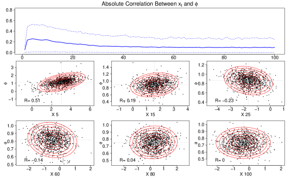
Moreover, the particles in the filter process are in fact coming from the marginal density $p(x_{t}|y^{t})$, not from the conditional density $p(x_{t}|\theta,y^{t})$. Reweighting particles using the transition density ignores the dependence between states and parameters, which causes inaccurate smoothing estimates when the dependency is strong. Figure 1 shows the dependency between the filtered samples of the states and parameters for the AR(1) plus noise model presented in Section 4. Correlations greater than 0.5 can be detected at the beginning of the time series. The simulation studies presented in Section 4 show that PLS gives poor smoothing estimates, particularly at early periods in the time series.

In the next section, we present two new smoothing algorithms. The first relies on a transformation of equation (4) and an adjustment of the weights in the backward pass to refine PLS. The second involves a separate forward-backward pass conditional on the sampled parameters.

Figure 1: AR(1) plus Noise Model. Top: means and 95% intervals for the posterior absolute correlation between state and AR coefficient $\phi$ at every time step $t$. Results are based on 500 simulated datasets. Middle and Bottom: posterior samples of $x_{t}$ and $\phi$ at selected time steps for one dataset. The contours represent the fitted normal densities used in the PLS_a algorithm.

3 Two New Smoothing Algorithms

3.1 PLS with Adjustment (PLS_a)

As stated earlier, the PLS algorithm assumes we have samples from the conditional distribution, $p(x_{t}|\theta,y^{t})$ in the filtering algorithm, when in fact we have samples from the joint, $p(x_{t},\theta|y^{t})$, and hence the marginal, $p(x_{t}|y^{t})$. Thus, the reweighting scheme in PLS does not give us samples from the target smoothing distribution. To provide a remedy for this, we consider the following rearrangement of equation (4):

$$\underbrace{p(x_{t}|x_{t+1},\theta,y^{t})}_{\text{smoother}}\propto\underbrace{p(x_{t+1}|x_{t},\theta)\;\dfrac{p(x_{t}|\theta,y^{t})}{p(x_{t}|y^{t})}}_{\text{weights}}\underbrace{p(x_{t}|y^{t})}_{\text{filter}}.$$ (5)

With samples from the filter, we use $\omega_{t}^{(j)}=p(x_{t+1}|x_{t}^{(j)},\theta)p(x_{t}^{(j)}|\theta,y^{t})/p(x_{t}^{(j)}|y^{t})$ as our resampling weights in the backward pass. Only in this way can we use the filtered particles in the smoothing algorithm. Note that, in most cases, we cannot compute these resampling weights exactly, since the joint filtering distribution $p(x_{t},\theta|y^{t})$ is generally not available in closed form. To fix this problem, we propose to use a multivariate normal approximation to $p(x_{t},\theta|y^{t})$ based on the filtered particles $\{(x_{t}^{(i)},\theta^{(i)})\}_{i=1}^{N}$, using appropriate transformations if necessary.

The algorithm proceeds exactly as in PLS, but with modified weights in the backward pass. The details of the particle learning and smoothing algorithm with adjustment (PLS_a) are presented below. Based on the simulation results in Section 4, we find that the adjustment of the weights matters: the adjusted version outperformed the original one significantly, especially in the beginning of the series, where the PLS usually has problems.

PLS_a Algorithm

1. (Forward Filter) Run a filtering and learning algorithm to obtain samples $\{(x_{t}^{(i)},\theta^{(i)})\}_{i=1}^{N}$ from $p(x_{t},\theta|y^{t})$ for $t=1,\ldots,T$. Use the filtered samples to construct a multivariate normal approximation at each time $t$:

   $$p(x_{t},\theta|y^{t})\approx\mathcal{N}\left(\begin{pmatrix}\mu_{t}^{x}\\ \mu_{t}^{\theta}\end{pmatrix},\begin{pmatrix}\Sigma_{t}^{x}&\Sigma_{t}^{x\theta}\\ \Sigma_{t}^{\theta x}&\Sigma_{t}^{\theta}\end{pmatrix}\right).$$

   This implies that the marginal and conditional distributions are also normal: $p(x_{t}|y^{t})\approx\mathcal{N}(\mu_{t}^{x},\Sigma_{t}^{x})$, and $p(x_{t}|\theta,y^{t})\approx\mathcal{N}(\mu_{t}^{x|\theta},\Sigma_{t}^{x|\theta}),$ where the conditional mean and covariance are given by the well-known formulas for multivariate normal distributions.

2. (Backward Smoother) Select a pair $(x_{T}^{(i)},\theta^{(i)})$ from Step 1, and simulate backwards: For $t$ = $T-1,\ldots,1$, resample the $\{x_{t}^{(j)}\}_{j=1}^{N}$ from Step 1 with weights proportional to

   $$\omega_{t}^{(j)}=p(x_{t+1}^{(i)}|x_{t}^{(j)},\theta^{(i)})\left(\frac{p(x_{t}^{(j)}|\theta^{(i)},y^{t})}{p(x_{t}^{(j)}|y^{t})}\right)\approx p(x_{t+1}^{(i)}|x_{t}^{(j)},\theta^{(i)})\left(\frac{\mathcal{N}(x_{t}^{(j)}|\mu_{t}^{x|\theta^{(i)}},\Sigma_{t}^{x|\theta})}{\mathcal{N}(x_{t}^{(j)}|\mu_{t}^{x},\Sigma_{t}^{x})}\right)$$

   to generate $x_{t}^{(i)}$.

3.2 Refiltering Smoothing Algorithm

In addition to the the PLS_a modification, we propose the following new smoothing algorithm. The idea is simple but proved to be efficient and accurate in simulation studies. The algorithm is based on the decomposition:

$$p(x^{T},\theta|y^{T})=p(x^{T}|y^{T},\theta)\;p(\theta|y^{T}).$$ (6)

We run Storvik’s forward filter, or more generally a filter method as in Liu and West (2001), to get samples of the parameter at the last time step, i.e. $\theta^{(i)}\sim p(\theta|y^{T})$. Then for each $\theta^{(i)}$, we apply a forward-backward smoothing algorithm as in Godsill et al. (2004) to get one state trajectory $x^{T(i)}$ from $p(x^{T}|y^{T},\theta^{(i)})$. Repeating this process for each $i$, we obtain states from the marginal smoothing density $p(x^{T}|y^{T})$.

Since the run time for the forward filter is negligible compared to the backward smoother, ($O(N)$ vs $O(N^{2})$, respectively), in simulation studies, we found that this algorithm almost has the same speed as PLS, but with significant improvement in accuracy. The algorithm is:

Refiltering Algorithm

1. (Forward Filter) Use Storvik, Particle Learning or Liu & West to run a forward filter and learning algorithm and generate $\theta^{(i)}\sim p(\theta|y^{T})$;

2. (Backward Smoother) For each $\theta^{(i)},i=1,\ldots,N_{0}$, run a forward-backward smoothing algorithm to get a sample $x^{T(i)}\sim p(x^{T}|y^{T},\theta^{(i)})$.

Note that this algorithm has a complexity of $O(TN^{2})$, the same as PLS. But we can make it an $O(TN)$ algorithm in two ways. The first one is that we can choose a small number of states $n_{0}\ll N$ for the forward-backward smoother in step 2. The second is to use a small number of parameter draws of size $N_{0}$ to use in step 2. The simulation study showed that both methods make the algorithm run much faster with only a minor loss of accuracy.

In the case where the model is linear and Gaussian: $x_{t}=G_{t}x_{t-1}+w_{t},\enspace w_{t}\sim\mathcal{N}(0,W)$; $y_{t}=F^{\prime}_{t}x_{t}+v_{t},\enspace v_{t}\sim\mathcal{N}(0,V)$; we can incorporate a forward filtering, backward sampling algorithm as in Carter and Kohn (1994) and Frühwirth-Schnatter (1994) into step 2 : we run a Kalman filter forward pass then generate a sample backwards based on equation $(3)$. Note $p(x_{t}|y^{t-1})\sim\mathcal{N}(a_{t},R_{t})$ is the prior and $p(x_{t}|y^{t})\sim\mathcal{N}(m_{t},C_{t})$ is the posterior of the state at each time point $t$, which depends on the parameters $\theta=(F_{t},G_{t},V,W)$.

Refiltering with FFBS

1. (Filter) Use Storvik, Particle Learning or Liu & West to run a forward filter and learning algorithm and generate $\theta^{(i)}\sim p(\theta|y^{T}),i=1,..,N$;

2. (Smoother) For each $\theta^{(i)},i=1,..,N_{0}$, run a Kalman filter and store prior and posterior moments $a_{t},R_{t},m_{t},C_{t}$. Sample $x_{T}^{(i)}\sim\mathcal{N}(m_{T},C_{T})$. For $t=T-1$ to 1, sample $x_{t}^{(i)}\sim p(x_{t}|x_{t+1}^{(i)},\theta^{(i)},y^{t})=\mathcal{N}(h_{t},H_{T})$, in which $h_{t}=m_{t}+B_{t}(x_{t+1}^{(i)}-a_{t+1})$, $H_{t}=C_{t}-B_{t}R_{t+1}B^{\prime}_{t}$ and $B_{t}=C_{t}G^{\prime}_{t+1}R^{-1}_{t+1}$. This provides a sample, $x^{T(i)}\sim p(x^{T}|y^{T},\theta^{(i)})$.

4 Examples

4.1 AR(1) Model with Three Unknown Parameters

Assume that the states $x_{t}$ follow an AR(1) process where the observations $y_{t}$ equal $x_{t}$ plus Gaussian noise:

$$x_{t}=\phi x_{t-1}+w_{t},\enspace w_{t}\sim\mathcal{N}(0,W),$$

$$y_{t}=x_{t}+v_{t},\enspace v_{t}\sim\mathcal{N}(0,V).$$

This benchmark model has been widely used in SMC and MCMC simulation studies (see, for example, Storvik, 2002; Polson, Stroud and Müller, 2008). In this model, FFBS can be easily implemented and a long chain MCMC with 150,000 iterations was set as a standard to compare with other smoothing algorithms. We generate $T=100$ observations with parameter values $V=W=1$, $\phi=0.75$ and $x_{0}=0$.

For the analysis, we assume conjugate priors for the parameters: $(\phi,W)\sim\mathcal{NIG}(b_{0},B_{0},n_{0},d_{0})$, and $V\sim\mathcal{IG}(\nu_{0},\delta_{0})$ where $\mathcal{IG}(a,b)$ denotes the inverse-gamma distribution with scale and shape parameters $a$ and $b$, and $\mathcal{NIG}$ denotes the normal-inverse gamma distribution where $B_{0}$ represents the inverse of the scale factor in the normal variance. We assume $n_{0}=\nu_{0}=d_{0}=\delta_{0}=2$ and $b_{0}=0.5,B_{0}=1$. The conjugate model for the parameters allows us to use Storvik’s algorithm, with the sufficient statistics $s_{t}=(b_{t},B_{t},n_{t},d_{t},\nu_{t},\delta_{t})$, and the updating recursions:

$$B_{t} =B_{t-1}+x_{t-1}^{2}, b_{t} =B_{t}^{-1}(B_{t-1}b_{t-1}+x_{t-1}x_{t}),$$

$$n_{t} =n_{t-1}+1/2, d_{t} =d_{t-1}+(b_{t-1}^{2}B_{t-1}+x_{t}^{2}-b_{t}^{2}B_{t})/2,$$

$$\nu_{t} =\nu_{t-1}+1/2, \delta_{t} =\delta_{t-1}+(y_{t}-x_{t})^{2}/2.$$

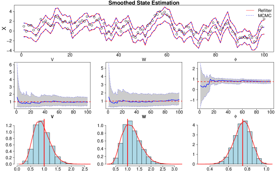
We first run Storvik’s filtering algorithm. Figure 2 shows the parameter learning plots and the posterior distribution at the last time period $T=100$. From the plot, we notice the true parameters values were learned properly and the samples of the parameters at the last time step are well concentrated around the true parameter values. Also the samples from the filter agree well with samples from a long MCMC. State smoothing by refiltering and the result of a long MCMC are also presented in Figure 2. We notice that the mean, $2.5^{th}$ and $97.5^{th}$ quantiles of the smoothing samples almost coincide for the two methods at each time step $t$.

Figure 2: AR(1) Plus Noise Model. Top: posterior mean and the $2.5^{th}$, $97.5^{th}$ quantiles based on the refiltering smoother (blue) and full MCMC (red). Middle: parameter learning in Storvik forward filter. Bottom: histograms of parameter samples at last filter step, superimposed with density estimation from long MCMC (red line). The true parameter values are indicated by horizontal and vertical red lines.

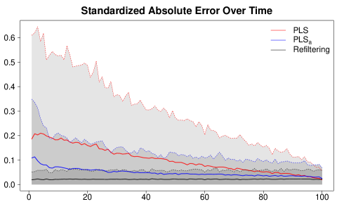
To show that PLS_a outperforms PLS using the same computation time, we ran 500 simulations for each of these two methods and compared the standardized absolute errors over time, i.e., $\hat{e}^{*}_{t}=|\hat{x_{t}}-\hat{x}^{true}_{t}|/\sigma(x_{t}|y^{T})$ for $t=1\dots T$, where $\hat{x}_{t}^{true}$ and $\sigma(x_{t}|y^{T})$ are the smoothed mean and standard deviation for $x_{t}$ computed from the long MCMC, and $\hat{x}_{t}$ is the smoothed mean from the other algorithms. The result is shown in Figure 3. From the plot, we can see the main difference between the two smoothing algorithms appears at the beginning of the series, in which the dependence of states and parameters is strong and therefore the adjustment matters. As time progresses, the dependency of states and parameters decreases, and the adjusted smoothing outcomes coincide with PLS. The results from the refiltering smoothing algorithm are also shown in the plot. For this model, refiltering substantially outperforms the other two methods, and its accuracy is consistent over time. Note that the number of particles for the three smoothing algorithms was adjusted to assure similar computation time.

Figure 3: AR(1) Plus Noise Model. Standardized absolute errors over time for three smoothing algorithms compared to a long MCMC. The results are based on 500 simulations. The long MCMC is treated as the truth. The solid lines are the means of standardized absolute errors at time $t$ among 500 simulations, while the dashed lines represent the $95^{th}$ quantile.

To compare the performance of all of the smoothing algorithms in this paper, we implement long and short MCMC runs, PLS, PLS_a, refiltering, $O(TN)$ refiltering, and refiltering with FFBS using 500 data simulations. All SMC based smoothing algorithms are run in parallel on 16 cores on a single node. Based on a similar run time, the mean standardized absolute errors over time (MAE* = $\sum_{t=1}^{T}|\hat{e}^{*}_{t}|/T$) are listed in Table 1. From the table, we see that the MAE* values for PLS_a are about half as large as for PLS. For all of the refiltering algorithms, the MAE* magnitude is only about one fifth of of that for PLS. Hence, both of the new smoothing algorithms outperform the PLS smoothing algorithm of Carvalho et al. (2010). The column labeled MAEP* represents the mean standardized absolute error between the posterior mean of the parameters at the last time step for a long MCMC versus the other algorithms. From the table, we see that the learning of parameters using the particle filter is almost as good as the learning from a short MCMC.

Table 1: Comparison of smoothing algorithms in AR(1) plus noise model. MAE* and MAEP* denote the standardized mean absolute error for the states and parameters, respectively. SMC smoothers are based on Storvik’s algorithm with $N=50,000$ particles.

Algorithm	$N(N_{0}/n_{0})$	Time	MAE*	MAEP*
MCMC	5000	17s	0.019	0.051
PLS	2300	22s	0.138	0.058
PLSa	1050	22s	0.060	0.058
Refiltering	1,500/1500	22s	0.026	0.058
Refiltering	10,000/150	22s	0.022	0.058
Refiltering	1,000/2500	23s	0.031	0.058
Refiltering/FFBS	44,000	21s	0.015	0.058

4.2 Nonstationary Growth Model with Five Unknown Parameters

Consider the nonstationary growth model:

$$x_{t} =\alpha x_{t-1}+\beta\frac{x_{t-1}}{1+x_{t-1}^{2}}+\gamma\cos(1.2(t-1))+w_{t},$$

$$y_{t} =x_{t}^{2}/20+v_{t},$$

in which $w_{t}\sim\mathcal{N}(0,W)$ and $v_{t}\sim\mathcal{N}(0,V)$. This benchmark nonlinear time series model has been used by Carlin et al. (1992) to test MCMC smoothing, by Gordon et al. (1993) to test the bootstrap filter, and by Briers et al. (2010) to test the Forward-Backward smoothing with known parameters. Here we test our smoothing methods on this model with unknown parameters.

We generate $T=100$ observations using parameter values $\alpha=0.5$, $\beta=25$ , $\gamma=8$, $V=5$ and $W=1$. We assume conjugate priors for the parameters similar to those given in Carlin et al. (1992), i.e. $((\alpha,\beta,\gamma)^{\prime},W)\sim\mathcal{NIG}(b_{0},B_{0},n_{0},d_{0})$, and $V\sim\mathcal{IG}(\nu_{0},\delta_{0})$, where $b_{0}=(0.5,25,8)^{\prime}$, $B_{0}=\text{diag}(1/0.25^{2},1/10^{2},1/4^{2})$, and $n_{0}=\nu_{0}=d_{0}=\delta_{0}=2$. The conjugate priors allow us to use Storvik’s algorithm for filtering and parameter learning. The updating recursions for the sufficient statistics are given by

$$B_{t} =B_{t-1}+F_{t}F_{t}^{\prime}, b_{t} =B_{t}^{-1}(B_{t-1}b_{t-1}+F_{t}x_{t}),$$

$$n_{t} =n_{t-1}+1/2, d_{t} =d_{t-1}+(b_{t-1}^{\prime}B_{t-1}b_{t-1}+x_{t}^{2}-b_{t}^{\prime}B_{t}b_{t})/2,$$

$$\nu_{t} =\nu_{t-1}+1/2, \delta_{t} =\delta_{t-1}+(y_{t}-x_{t}^{2}/20)^{2}/2,$$

where $F_{t}=(x_{t-1},x_{t-1}/(1+x_{t-1}^{2}),\cos(1.2(t-1))$. The parameter learning process and the posterior histograms of the parameters at time $T=100$ are plotted in Figure 4. In the figure, the 95% confidence bands narrow down quickly as time increases. In the histograms, the samples concentrate around the true parameter values. A total of $N=50,000$ particles were used for the forward pass.

Furthermore, we compare the refiltering smoothing algorithm using $N_{0}=5000$ and $n_{0}=1000$, with a long MCMC using $N=150,000$ iterations. The smoothing plot is also presented in Figure 4. The results from the two smoothing algorithms closely agree with each other.

Figure 4: Nonlinear Model. Top: refiltering smoothing compared with MCMC. Middle: parameter learning in Storvik forward filter. Bottom: histogram of parameter samples at last filter step, superimposed with density estimation from long MCMC (red line).

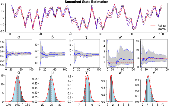
Table 2 gives a summary of the overall performance of the three smoothing algorithms compared to a long MCMC, using 500 simulated datasets. A decrease in the mean absolute error for the new methods relative to PLS is obvious. The plot of the standardized absolute errors over time of the three smoothing algorithms (not shown) illustrates the same patterns as for the AR(1) model: the main improvement of the two new smoothing algorithms over PLS is evident at the beginning of the time series.

Note that for this model, it is difficult to distinguish between the positive and negative sign of the states based on the data, thus it is difficult to assign initial values for the states for the MCMC algorithm based on observations. With a bad starting values for the states, the MCMC chain takes much longer to converge. In contrast, smoothing based on SMC does not suffer from the initialization problem.

Table 2: Comparison of smoothing algorithms for the nonlinear growth model. SMC smoothers are based on Storvik’s algorithm with $N=50,000$ (run time 96s).

Algorithm	$N(N_{0}/n_{0})$	Time	MAE*	MAEP*
MCMC	20000	228s	0.075	0.246
PLS	10000	200s	0.373	0.213
PLSa	5000	208s	0.189	0.213
Refiltering	5000/1000	231s	0.097	0.213

4.3 Chaotic Model with Three Unknown Parameters

Now let us consider data generated from the model:

$$N_{t} =rN_{t-1}e^{-N_{t-1}+z_{t}},\enspace z_{t}\sim\mathcal{N}(0,\sigma^{2}),$$

$$y_{t} \sim Pois(\phi N_{t}).$$

This model is widely used in the field of ecology (Fasiolo, Pya and Wood, 2016), where $N_{t}$ stands for the density of the population at generation $t$, and $r$ is the growth rate of the population. This model is characterized by its sensitivity to parameter variations: small increments in $r$ will lead to significant oscillations in the likelihood function. As a result, parameter estimation via maximum likelihood methods is challenging. Fasiolo, Pya and Wood (2016) described the pathological likelihood function for this model and compared the performance of information reduction approaches and state-space methods for this model. A time series of 100 observations is generated from this model with true parameter values $r=e^{3.8}$, $\sigma^{2}=0.3$ and $\phi=10$.

To estimate this model using our framework, we first make the transformations, $x_{t}=\log(N_{t})$ and $\mu=\log(r)$. Then the system and observation equations become

$$x_{t} =\mu+x_{t-1}-e^{x_{t-1}}+z_{t},$$

$$y_{t} \sim Pois(\phi e^{x_{t}}).$$

We assume diffuse conjugate priors for the parameters of the form, $\phi\sim\mathcal{G}(a_{0},b_{0});$ and $(\mu,\sigma^{2})\sim\mathcal{NIG}(m_{0},c_{0},n_{0},d_{0})$, where $\mathcal{G}$ denotes the gamma distribution, with $a_{0}=15,b_{0}=1,m_{0}=5,c_{0}=.1,n_{0}=2,d_{0}=2$. The sufficient statistics are $s_{t}=(a_{t},b_{t},m_{t},c_{t},n_{t},d_{t})$, and the updating recursions are

$$a_{t} =a_{t-1}+y_{t}, b_{t} =b_{t-1}+e^{x_{t}},$$

$$c_{t} =c_{t-1}+1, m_{t} =c_{t}^{-1}(c_{t-1}m_{t-1}+x_{t}-x_{t-1}+e^{x_{t-1}}),$$

$$n_{t} =n_{t-1}+1/2, d_{t} =d_{t-1}+\{c_{t-1}m_{t-1}^{2}+(x_{t}-x_{t-1}+e^{x_{t-1}})^{2}-c_{t}m_{t}^{2}\}/2.$$

The parameter learning process is summarized in Figure 5. A total of $N=50,000$ particles were used for the filtering. The true parameter values were learned quickly and the posterior samples of the parameters settle around the true values. Figure 5 also provides a comparison of refiltering with $N_{0}=5000$ and $n_{0}=1000$ to a long MCMC with 150,000 iterations for smoothing, which shows similar results for both methods.

Figure 5: Chaotic Model. Top: refilter smoothing compared with MCMC. Middle: parameter learning in Storvik forward filter process. Bottom: histogram of parameter samples at last filter step, superimposed with density estimation from long MCMC (red line).

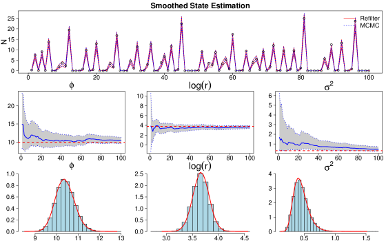
To allow a comparison of the three smoothing methods, 100 simulations were performed. We examined plots of the MAE* values over time (not shown), and Table 3 presents numerical summaries based on the simulations. From the plots, we find similar patterns for this example as in the previous two: PLS_a and refiltering dominate PLS early in the time series (up to about time $t=80$), and the three methods coincide afterwards. From Table 3, we notice a decrease in MAE* for the two new methods compared to PLS. We also find that smoothing method based on refiltering performs better compared to a short MCMC for this model.

Table 3: Comparison of smoothing algorithms for the chaotic model. SMC smoothers are based on Storvik’s algorithm with $N=50,000$ (run time 11s).

Algorithm	$N(N_{0}/n_{0})$	Time	MAE*	MAEP*
MCMC	30000	184s	0.097	0.166
PLS	10000	219s	0.190	0.206
PLSa	5000	180s	0.108	0.206
Refiltering	5000/1000	40s	0.089	0.206

4.4 Analysis of S&P 500 Returns

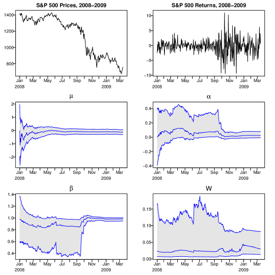
In this section, we analyze daily returns on the S&P 500 index from January 2008 to March 2009, during the financial crisis, and compare the PLS, PLS_a and refiltering smoothers with MCMC where daily returns $y_{t}$ follow a stochastic volatility model:

$$x_{t} =\alpha+\beta x_{t-1}+\omega_{t},\enspace\omega_{t}\sim\mathcal{N}(0,W),$$

$$y_{t} =\mu+\exp(x_{t}/2)v_{t},\enspace v_{t}\sim\mathcal{N}(0,1).$$

Here $y_{t}=\log(P_{t}/P_{t-1})$ are the daily returns, $P_{t}$ are the prices, $\mu$ is the expected return, and $x_{t}$ is the unobserved log-variance at time $t$, which is assumed to follow an AR(1) model with drift $\alpha$. The AR coefficient $\beta$ measures the autocorrelation present in the logged squared data. This model has been widely used to analyze financial time series with volatility clustering (see, for example, Jacquier, Polson and Rossi, 1994; Kim, Shephard and Chib, 1998).

We assume conjugate priors for the parameters $\theta=(\mu,\alpha,\beta,W)$. For the expected returns, $\mu\sim\mathcal{N}(a_{0},b_{0})$, and for the volatility parameters, we assume $((\alpha,\beta)^{\prime},W)\sim\mathcal{NIG}(m_{0},C_{0},n_{0},d_{0})$, where $a_{0}=0,b_{0}=1,m_{0}=(0,.9)^{\prime},C_{0}=\mbox{diag}(1,1),n_{0}=2,d_{0}=2$. The refiltering algorithm is implemented with $N=10,000$ and $n_{0}=1000$. The parameter learning and state smoothing estimates are compared to an MCMC with 15,000 iterations, using the single-state updating scheme of Jacquier et al. (1994).

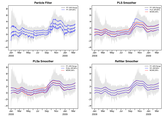
From the sequential learning plots in Figure 6, a significant change in the parameters is observed in September 2008, especially for $\alpha$ and $\beta$. The change corresponds to the collapse of Lehman Brothers, and an increase in the volatility of the index. Figure 7 shows the filtered and smoothed volatilities for each algorithm. These plots show clear evidence that PLS and MCMC do not match, especially from September-November 2008, when the volatility changes abruptly. PLS_a reduces this discrepancy somewhat, and among the three new smoothing algorithms, refiltering is by far the most accurate. Given that the run times for refiltering and MCMC are roughly the same, and the close match between the corresponding posterior distributions, we conclude that these two algorithms are comparable.

Figure 6: Stochastic Volatility Model. Top row: Daily prices and returns on the S&P 500 index from January 2008 to March 2009. Middle and bottom rows: filtered medians and 95% intervals for the parameters $\mu$, $\alpha$, $\beta$ and $W$. Based on Storvik’s algorithm with 50,000 particles.

Figure 7: Stochastic Volatility Model. Top left: filtered median and 95% posterior intervals for $x_{t}$ from Storvik’s algorithm. The other three panels show the smoothed median and 95% intervals for $x_{t}$ using MCMC and the PLS, PLS_a and refiltering algorithms. The gray bands in each plot are the 100% filtering intervals (i.e., range) from Storvik’s algorithm.

5 Conclusions

In this paper, we proposed two new SMC-based smoothing algorithms that simultaneously deal with parameter learning. The first is a modification of the PLS algorithm of Carvalho et al. (2010), that adds a correction term in the backward resampling weights. The second is a two-step algorithm, called refiltering, that includes a parameter learning step followed by a forward-backward algorithm for smoothing. Refiltering is well suited for parallel implementation, since the smoothing step requires essentially no communication between processors. We tested the new methods on four models: a benchmark AR(1) plus noise model, a nonlinear growth model, a chaotic model from ecology, and a stochastic volatility model from finance, and compared the estimates with the widely-used smoothing method known as PLS. For all examples, both new methods showed significant improvement over PLS, and refiltering was competitive with MCMC. Overall, our proposed methods are quite general, and may be applied to a wide class of state-space models for parameter and state estimation. In future work, we plan to apply the methods to other real data applications in finance and ecology.

Appendix A: Marginal Likelihood of the Model

The marginal likelihood is important in Bayesian model selection. As noted by Carvalho et al. (2010), the marginal likelihood can be computed trivially from the output of SMC-based Bayesian filtering and learning algorithms (e.g., Storvik, 2002; Carvalho et al., 2010). Define $\omega_{t}^{j}=p(y_{t}|x_{t}^{j},\theta^{j},\mathcal{M})$, where $(x_{t}^{j},\theta^{j})\sim p(x_{t},\theta|y^{t-1},\mathcal{M})$ for given model $\mathcal{M}$. Then, the log marginal likelihood for model $\mathcal{M}$ is estimated by

$$\log(f(y|\mathcal{M}))\approx\sum_{t=1}^{T}\log\left(\sum_{j=1}^{N}\omega_{t}^{j}\right)-T\log(N).$$

By comparison, many different MCMC-based estimates of the marginal likelihood have been proposed. One of the most commonly used and straightforward methods is the harmonic mean estimator (Newton and Raftery, 1994), which can be computed based on the joint distribution of the data:

$$\log(f(y|\mathcal{M}))\approx\log\left(\dfrac{1}{\frac{1}{N}\sum_{j=1}^{N}\frac{1}{p(y|\psi^{j},\mathcal{M})}}\right),$$

where $y=(y_{1},\ldots,y_{T})$ are the observations, $N$ is the total number of MCMC iterations, and $\psi^{j}=(x^{j},\theta^{j}),j=1,\ldots,N$ are the posterior draws of the states and parameters.

An important advantage of SMC over MCMC is that the estimation of marginal likelihood from SMC output is stable. As shown in Table 4, in our simulation studies, we find that the SMC-based marginal likelihood estimator converges quickly as $N$ increases, while for MCMC, the harmonic mean estimator fails to converge even for $N$ larger than 500K in all three models.

Table 4: Comparison of Log Likelihood

		AR(1) + Noise			Nonlinear Growth			Chaotic Model
$N$		Storvik	MCMC		Storvik	MCMC		Storvik	MCMC
1K		-176.44	-164.40		-212.91	-253.27		-286.34	-193.37
5K		-176.71	-171.74		-212.51	-169.92		-284.88	-200.35
10K		-176.71	-169.88		-211.66	-170.42		-284.96	-195.64
50K		-176.87	-169.86		-212.45	-170.91		-285.16	-199.54
100K		-176.91	-170.84		-212.10	-162.56		-284.98	-196.61
500K		-176.88	-173.56		-212.30	-164.06		-285.10	-197.99

References

- Briers et al. (2010) Briers, M., Doucet, A. and Maskell, S. (2010) Smoothing algorithms for state-space models. Annals of the Institute of Statistical Mathematics, 62, 61–89.
- Carlin et al. (1992) Carlin, B. P., Polson, N. G. and Stoffer, D. S. (1992) A Monte Carlo approach to nonnormal and nonlinear state-space modeling. Journal of the American Statistical Association, 87, 493–500.
- Carter and Kohn (1994) Carter, C. K. and Kohn, R. (1994) On Gibbs sampling for state space models. Biometrika, 81, 541–553.
- Carvalho et al. (2010) Carvalho, C. M., Johannes, M. S., Lopes, H. F. and Polson, N. G. (2010) Particle learning and smoothing. Statistical Science, 25, 88–106.
- Fasiolo et al. (2016) Fasiolo, M., Pya, N. and Wood, S. N. (2016) A comparison of inferential methods for highly non-linear state space models in ecology and epidemiology. Statistical Science, 31, 96–118.
- Fearnhead (2002) Fearnhead, P. (2002) Markov chain Monte Carlo, sufficient statistics, and particle filters. Journal of Computational and Graphical Statistics, 11, 848–862.
- Fearnhead et al. (2010) Fearnhead, P., Wyncoll, D. and Tawn, J. (2010) A sequential smoothing algorithm with linear computational cost. Biometrika, 97, 447–464.
- Frühwirth-Schnatter (1994) Frühwirth-Schnatter, S. (1994) Data augmentation and dynamic linear models. Journal of Time Series Analysis, 15, 183–202.
- Gamerman (1998) Gamerman, D. (1998) Markov chain Monte Carlo for dynamic generalized linear models. Biometrika, 85, 215–227.
- Geweke and Tanizaki (2001) Geweke, J. and Tanizaki, H. (2001) Bayesian estimation of state-space models using the Metropolis–Hastings algorithm within Gibbs sampling. Computational Statistics and Data Analysis, 37, 151 – 170.
- Godsill et al. (2004) Godsill, S. J., Doucet, A. and West, M. (2004) Monte Carlo smoothing for nonlinear time series. Journal of the American Statistical Association, 99, 156–168.
- Gordon et al. (1993) Gordon, N. J., Salmond, D. J. and Smith, A. F. M. (1993) Novel approach to nonlinear/non-Gaussian Bayesian state estimation. IEE Proceedings F, Radar and Signal Processing, 140, 107–113.
- Jacquier et al. (1994) Jacquier, E., Polson, N. G. and Rossi, P. E. (1994) Bayesian analysis of stochastic volatility models. Journal of Economic and Business Statistics, 12, 371–417.
- de Jong and Shephard (1995) de Jong, P. and Shephard, N. (1995) The simulation smoother for time series models. Biometrika, 82, 339–350.
- Kantas et al. (2015) Kantas, N., Doucet, A., Singh, S. S., Maciejowski, J. and Chopin, N. (2015) On particle methods for parameter estimation in state-space models. Statistical Science, 30, 328–351.
- Kim et al. (1998) Kim, S., Shephard, N. and Chib, S. (1998) Stochastic volatility: Likelihood inference and comparison with ARCH models. Review of Economic Studies, 65, 361–393.
- Kitagawa (1996) Kitagawa, G. (1996) Monte Carlo filter and smoother for non-Gaussian nonlinear state space models. Journal of Computational and Graphical Statistics, 5, 1–25.
- Kitagawa (1998) — (1998) A self-organizing state-space model. Journal of the American Statistical Association, 93, 1203–1215.
- Kitagawa and Sato (2001) Kitagawa, G. and Sato, S. (2001) Monte Carlo smoothing and self-organising state-space model. Statistics for Engineering and Information Science, 177–195. Springer:New York.
- Liu and West (2001) Liu, J. and West, M. (2001) Combined parameter and state estimation in simulation-based filtering. In Sequential Monte Carlo Methods in Practice (eds. A. Doucet, N. de Freitas and N. Gordon), Statistics for Engineering and Information Science, 197–223. Springer:New York.
- Newton and Raftery (1994) Newton, M. A. and Raftery, A. E. (1994) Approximate Bayesian inference with the weighted likelihood bootstrap (with discussion). Journal of the Royal Statistical Society, Series B (Statistical Methodology), 56, 3–48.
- Niemi and West (2010) Niemi, J. and West, M. (2010) Adaptive mixture modeling Metropolis methods for Bayesian analysis of nonlinear state-space models. Journal of Computational and Graphical Statistics, 19, 260–280.
- Pitt and Shephard (1999) Pitt, M. and Shephard, N. (1999) Filtering via simulation: Auxiliary particle filters. Journal of the American Statistical Association, 94, 590–599.
- Polson et al. (2008) Polson, N. G., Stroud, J. R. and Müller, P. (2008) Practical filtering with sequential parameter learning. Journal of the Royal Statistical Society, Series B (Statistical Methodology), 70, 413–428.
- Shephard and Pitt (1997) Shephard, N. and Pitt, M. K. (1997) Likelihood analysis of non-Gaussian measurement time series. Biometrika, 84, 653–667.
- Storvik (2002) Storvik, G. (2002) Particle filters for state-space models with the presence of unknown static parameters. IEEE Transactions on Signal Processing, 50, 281–289.
- Stroud et al. (2003) Stroud, J. R., Müller, P. and Polson, N. G. (2003) Nonlinear state-space models with state-dependent variances. Journal of the American Statistical Association, 98, 377–386.