Decentralized Consensus Algorithm with Delayed and Stochastic Gradients

Abstract

We analyze the convergence of decentralized consensus algorithm with delayed gradient information across the network. The nodes in the network privately hold parts of the objective function and collaboratively solve for the consensus optimal solution of the total objective while they can only communicate with their immediate neighbors. In real-world networks, it is often difficult and sometimes impossible to synchronize the nodes, and therefore they have to use stale gradient information during computations. We show that, as long as the random delays are bounded in expectation and a proper diminishing step size policy is employed, the iterates generated by decentralized gradient descent method converge to a consensual optimal solution. Convergence rates of both objective and consensus are derived. Numerical results on a number of synthetic problems and real-world seismic tomography datasets in decentralized sensor networks are presented to show the performance of the method.

Key words. Decentralized consensus, delayed gradient, stochastic gradient, decentralized networks.

AMS subject classifications. 65K05, 90C25, 65Y05.

1 Introduction

In this paper, we consider a decentralized consensus optimization problem arising from emerging technologies such as distributed machine learning [3, 10, 16, 19], sensor network [13, 30, 36], and smart grid [11, 21]. Let $\mathcal{G}=(\mathcal{V},\mathcal{E})$ be a network (undirected graph) where $\mathcal{V}=\{1,2,\dots,m\}$ is the node (also called agent, processor, or sensor) set and $\mathcal{E}\subset\mathcal{V}\times\mathcal{V}$ is the edge set. Two nodes $i$ and $j$ are called neighbors if $(i,j)\in\mathcal{E}$. The communications between neighbor nodes are bidirectional, meaning that $i$ and $j$ can communicate with each other as long as $(i,j)\in\mathcal{E}$.

In a decentralized sensor network $\mathcal{G}$, individual nodes can acquire, store, and process data about large-sized objects. Each node $i$ collects data and holds objective function $F_{i}(x;\xi_{i})$ privately where $\xi_{i}\in\Theta$ is random with fixed but unknown probability distribution in domain $\Theta$ to model environmental fluctuations such as noise in data acquisition and/or inaccurate estimation of objective function or its gradient. Here $x\in X$ is the unknown (e.g., the seismic image) to be solved, where the domain $X\subset\mathbb{R}^{n}$ is compact and convex. Furthermore, we assume that $F_{i}(\cdot;\xi_{i})$ is convex for all $\xi_{i}\in\Theta$ and $i\in\mathcal{V}$, and we define $f_{i}(x)=\operatorname{\mathbb{E}}_{\xi_{i}}[F_{i}(x;\xi_{i})]$ which is thus convex with respect to $x\in X$. The goal of decentralized consensus optimization is to solve the minimization problem

$$\mathop{\rm minimize}_{x\in X}f(x),\quad\mbox{where}\ f(x)\mathrel{\mathop{\mathchar 58\relax}}=\sum_{i=1}^{m}f_{i}(x)$$ (1)

with the restrictions that $F_{i}(x;\xi_{i})$, and hence $f_{i}(x)$, are accessible by node $i$ only, and that nodes $i$ and $j$ can communicate only if $(i,j)\in\mathcal{E}$ during the entire computation.

There are a number of practical issues that need to be taken into consideration in solving the real-world decentralized consensus optimization problem (1):

• The partial objective $F_{i}$ (and $f_{i}$) is held privately by node $i$, and transferring $F_{i}$ to a data fusion center is either infeasible or cost-ineffective due to data privacy, the large size of $F_{i}$, and/or limited bandwidth and communication power overhead of sensors. Therefore, the nodes can only communicate their own estimates of $x\in\mathbb{R}^{n}$ with their neighbors in each iteration of a decentralized consensus algorithm.

• Since it is often difficult and sometimes impossible for the nodes to be fully synchronized, they may not have access to the most up-to-date (stochastic) gradient information during computations. In this case, the node $i$ has to use out-of-date (stochastic) gradient $\nabla F_{i}(x_{i}(t-\tau_{i}(t));\xi_{i}(t-\tau_{i}(t)))$ where $x_{i}(t)$ is the estimate of $x$ obtained by node $i$ at iteration $t$, and $\tau_{i}(t)$ is the level of (possibly random) delay of the gradient information at $t$.

• The estimates $\{x_{i}(t)\}$ by the nodes should tend to be consensual as $t$ increases, and the consensual value is a solution of problem (1). In this case, there is a guarantee of retrieving a good estimate of $x$ from any surviving node in the network even if some nodes are sabotaged, lost, or run out of power during the computation process.

In this paper, we analyze a decentralized consensus algorithm which takes all the factors above into consideration in solving (1). We provide comprehensive convergence analysis of the algorithm, including the decay rates of objective function and disagreements between nodes, in terms of iteration number, level of delays, and network structure etc.

1.1 Related work

Distributed computing on networks is an emerging technology with extensive applications in modern machine learning [10, 16, 19], sensor networks [13, 30, 49, 50], and big data analysis [4, 31]. There are two types of scenarios in distributed computing: centralized and decentralized. In the centralized scenario, computations are carried out locally by worker (slave) nodes while computations of certain global variables must eventually be processed by designated master node or at a center of shared memory during each (outer) iteration. A major effort in this scenario has been devoted to update the global variable more effectively using an asynchronous setting in, for example, distributed centralized alternating direction method of multipliers (ADMM) [7, 5, 20, 42, 47]. In the decentralized scenario considered in this paper, the nodes privately hold parts of objective functions and can only communicate with neighbor nodes during computations. In many real-world applications, decentralized computing is particularly useful when a master-worker network setting is either infeasible or not economical, or the data acquisition and computation have to be carried out by individual nodes which then need to collaboratively solve the optimization problem. Decentralized networks are also more robust to node failure and can better address privacy concerns. For more discussions about motivations and advantages of decentralized computing, see, e.g., [15, 27, 29, 34, 38, 40] and references therein.

Decentralized consensus algorithms take the data distribution and communication restriction into consideration, so that they can be implemented at individual nodes in the network. In the ideal synchronous case of decentralized consensus where all the nodes are coordinated to finish computation and then start to exchange information with neighbors in each iteration, a number of developments have been made. A class of methods is to rewrite the consensus constraints for minimization problem (1) by introducing auxiliary variables between neighbor nodes (i.e., edges), and apply ADMM (possibly with linearization or preconditioning techniques) to derive an implementable decentralized consensus algorithm [6, 12, 14, 23, 35, 46]. Most of these methods require each node to solve a local optimization problem every iteration before communication, and reach a convergence rate of $O(1/T)$ in terms of outer iteration (communication) number $T$ for general convex objective functions $\{f_{i}\}$. First-order methods based on decentralized gradient descent require less computational cost at individual nodes such that between two communications they only perform one step of a gradient descent-type update at the weighted average of previous iterates obtained from neighbors. In particular, Nesterov’s optimal gradient scheme is employed in decentralized gradient descent with diminishing step sizes to achieve rate of $O(1/T)$ in [15], where an alternative gradient method that requires excessive communications in each inner iteration is also developed and can reach a theoretical convergence rate of $O(\log T/T^{2})$, despite that it seems to work less efficiently in terms of communications than the former in practice. A correction technique is developed for decentralized gradient descent with convergence rate as $O(1/T)$ with constant step size in [34], which results in a saddle-point algorithm as pointed out in [24]. In [50], the authors combine Nesterov’s gradient scheme and a multiplier-type auxiliary variable to obtain a fast optimality convergence rate of $O(1/T^{2})$. Other first-order decentralized methods have also been developed recently, such dual averaging [8]. Additional constraints for primal variables in decentralized consensus optimization (1) are considered in [45].

In real-world decentralized computing, it is often difficult and sometimes impossible to coordinate all the nodes in the network such that their computation and communication are perfectly synchronized. One practical approach for such asynchronous consensus is using a broadcast scenario where in each (outer) iteration, one node in the network is assumed to wake up at random and broadcasts its value to neighbors (but does not hear them back). A number of algorithms for broadcast consensus are developed, for instance, in [2, 13, 25, 26]. In particular, [26] develops a consensus optimization algorithm for (1) in the setting where every iteration one node in the network broadcasts its value to the neighbors, but there are no delays in (sub)gradients during their updates. Another important issue in the asynchronous setting is that nodes may have to use out-of-date (stale) gradient information during updates [27, 43]. This delayed scenario in gradient descent is considered in a distributed but not decentralized setting in [1, 18, 37, 48]. In addition, analysis of stochastic gradient in distributed computing is also carried out in [1, 33]. In [9], linear convergence rate of optimality is derived for strongly convex objective functions with delays. Extending [1], a fixed delay at all nodes is considered in dual averaging [17] and gradient descent [41] in a decentralized setting, but they did not consider more practical and useful random delays, and there are no convergence rates on node consensus provided in these papers. In [43], both random delays in communications and gradients are considered, however, no convergence rate is established in such setting.

1.2 Contributions

The contribution of this paper is in three phases.

First, we consider a general decentralized consensus algorithm with randomly delayed and stochastic gradient (Section 2). In this case, the nodes do not need to be synchronized and they may only have access to stale gradient information. This renders stochastic gradients with random delays at different nodes in their gradient updates, which is suitable for many real-world decentralized computing applications.

Second, we provide a comprehensive convergence analysis of the proposed algorithm (Section 3). More precisely, we derive convergence rates for both the objective function (optimality) and disagreement (feasibility constraint of consensus), and show their dependency on the characteristics of the problem, such as Lipschitz constants of (stochastic) gradients and spectral gaps of the underlying network.

Third, we conduct a number of numerical experiments on synthetic and real datasets to validate the performance of the proposed algorithm (Section 4). In particular, we examine the convergence on synthetic decentralized least squares, robust least squares, and logistic regression problems. We also present the numerical results on the reconstruction of several seismic images in decentralized wireless sensor networks.

1.3 Notations and assumptions

In this paper, all vectors are column vectors unless otherwise noted. We denote by $x_{i}(t)\in\mathbb{R}^{n}$ the estimate of node $i$ at iteration $t$, and $x(t)=(x_{1}(t),\dots,x_{m}(t))^{\top}\in\mathbb{R}^{m\times n}$. We denote $\|x\|\equiv\|x\|_{2}$ if $x$ is a vector and $\|x\|\equiv\|x\|_{F}$ if $x$ is a matrix, which should be clear by the context. For any two vectors of same dimension, $\langle x,y\rangle$ denotes their inner product, and $\langle x,y\rangle_{Q}\mathrel{\mathop{\mathchar 58\relax}}=\langle x,Qy\rangle$ for symmetric positive semidefinite matrix $Q$. For notation simplicity, we use $\langle x,y\rangle=\sum_{i=1}^{m}\langle x_{i},y_{i}\rangle$ where $x_{i}$ and $y_{i}$ are the $i$-th row of the $m\times n$ matrices $x$ and $y$ respectively. Such matrix inner product is also generalized to $\langle x,y\rangle_{Q}$ for matrices $x$ and $y$. In this paper, we set the domain $X\mathrel{\mathop{\mathchar 58\relax}}=\{x\in\mathbb{R}^{n}\mathrel{\mathop{\mathchar 58\relax}}\|x\|_{\infty}\leq R\}$ for some $R>0$, which can be thought of as the maximum pixel intensity in reconstructed images for instance. We further denote $\mathcal{X}\mathrel{\mathop{\mathchar 58\relax}}=X^{m}\subset\mathbb{R}^{m\times n}$.

For each node $i$, we define $f_{i}(x)\mathrel{\mathop{\mathchar 58\relax}}=\operatorname{\mathbb{E}}_{\xi_{i}}[F_{i}(x;\xi_{i})]$ as the expectation of objective function, and $g_{i}(t)\mathrel{\mathop{\mathchar 58\relax}}=\nabla F_{i}(x(t);\xi_{i}(t))$ (here the gradient $\nabla$ is taken with respect to $x$) is the stochastic gradient at $x_{i}(t)$ at node $i$. We let $\tau_{i}(t)$ be the delay of gradient at node $i$ in iteration $t$, and $\tau(t)=(\tau_{1}(t),\dots,\tau_{m}(t))^{\top}$. We write $f(x(t))$ in short for $\sum_{i=1}^{m}f_{i}(x_{i}(t))\in\mathbb{R}$, $x(t-\tau(t))$ for $(x_{1}(t-\tau_{1}(t)),\dots,x_{m}(t-\tau_{m}(t)))^{\top}\in\mathbb{R}^{m\times n}$, and $g(t-\tau(t))$ for $(g_{1}(t-\tau_{1}(t)),\dots,g_{m}(t-\tau_{m}(t)))^{\top}\in\mathbb{R}^{m\times n}$. We assume $f_{i}$ is continuously differentiable, $\nabla f_{i}$ has Lipschitz constant $L_{i}$, and denote $L\mathrel{\mathop{\mathchar 58\relax}}=\max_{1\leq i\leq m}L_{i}$.

Let $x^{*}\in\mathbb{R}^{n}$ be a solution of (1), we denote $\mathbf{1}(x^{*})^{\top}$ simply by $x^{*}$ in this paper which is clear by the context, for instance $f(x^{*})=f(\mathbf{1}(x^{*})^{\top})=\sum_{i=1}^{m}f_{i}(x^{*})$. Furthermore, we let $y(T)\mathrel{\mathop{\mathchar 58\relax}}=(1/T)\sum_{t=1}^{T}x(t+1)$ be the running average of $\{x(t+1)\mathrel{\mathop{\mathchar 58\relax}}1\leq t\leq T\}$, and $z(T)\mathrel{\mathop{\mathchar 58\relax}}=(1/m)\sum_{i=1}^{m}y(T)$ be the consensus average of $y(T)$. We denote $J=(1/m)\mathbf{1}\mathbf{1}^{\top}$, then $z(T)=Jy(T)$. Note that for all $T$, $z(T)$ is always consensual but $x(T),y(T)$ may not be.

An important ingredient in decentralized gradient descent is the mixing matrix $W=[w_{ij}]$ in (2). For the algorithm to be implementable in practice, $w_{ij}>0$ if and only if $(i,j)\in\mathcal{E}$. In this paper, we assume that $W$ is symmetric and $\sum_{j=1}^{m}w_{ij}=1$ for all $i$, hence $W$ is doubly stochastic, namely $W\mathbf{1}=\mathbf{1}$ and $\mathbf{1}^{\top}W=\mathbf{1}^{\top}$ where $\mathbf{1}=(1,\dots,1)^{\top}\in\mathbb{R}^{m}$. With the assumption that the network $\mathcal{G}$ is simple and connected, we know $\|W\|_{2}=1$ and eigenvalue $1$ of $W$ has multiplicity $1$ by the Perron-Frobenius theorem [22]. As a consequence, $Wx=x$ if and only if $x$ is consensual, i.e., $x=c\mathbf{1}$ for some $c\in\mathbb{R}$. We further assume $W\succeq 0$ (otherwise use $\frac{1}{2}(I+W)\succeq 0$ since stochastic matrix $W$ has spectral radius 1). Given a network $\mathcal{G}$, there are different ways to design the mixing matrix $W$. For some optimal choices of $W$, see, e.g., [32, 44].

Now we make several assumptions that are necessary in our convergence analysis.

1. The network $\mathcal{G}=(\mathcal{V},\mathcal{E})$ is undirected, simple, and connected.

2. For all $i$ and $x$, the stochastic gradient is unbiased, i.e., $\operatorname{\mathbb{E}}_{\xi_{i}}[\nabla F_{i}(x;\xi_{i})]=\nabla f_{i}(x)$, and $\operatorname{\mathbb{E}}_{\xi_{i}}[\|\nabla F_{i}(x;\xi_{i})-\nabla f_{i}(x)\|^{2}]\leq\sigma^{2}$ for some $\sigma>0$.

3. The delays $\tau_{i}(t)$ may follow different distributions at different nodes, but their second moments are assumed to be uniformly bounded, i.e., there exists $B>0$ such that $\operatorname{\mathbb{E}}[\tau_{i}(t)^{2}]\leq B^{2}$ for all $i=1,\dots,m$ and iteration $t$.

Since the domain $X$ is compact and $\nabla f_{i}$ are all Lipschitz continuous, we know $\|\nabla f_{i}\|$ is uniformly bounded. Furthermore, $\operatorname{\mathbb{E}}[\|\nabla F_{i}(\cdot,\xi_{i})\|]\leq\operatorname{\mathbb{E}}[\|\nabla F_{i}(\cdot,\xi_{i})-\nabla f_{i}(\cdot)\|]+\|\nabla f_{i}(\cdot)\|\leq\sigma+\|\nabla f_{i}(\cdot)\|$, we know $\operatorname{\mathbb{E}}[\|\nabla F_{i}(\cdot,\xi_{i})\|]$ is also uniformly bounded. Therefore, we denote by $G>0$ the uniform bound such that $\|\nabla f_{i}\|,\operatorname{\mathbb{E}}[\|\nabla F_{i}(\cdot,\xi_{i})\|]\leq G$ for all $i$. We also assume that the random delay $\tau_{i}(t)$ and error of inexact gradient $\epsilon_{i}(t)\mathrel{\mathop{\mathchar 58\relax}}=g_{i}(t)-\nabla f_{i}(x(t))$ are independent.

2 Algorithm

Taking the delayed stochastic gradient and the constraint that nodes can only communicate with immediate neighbors, we propose the following decentralized delayed stochastic gradient descent method for solving (1). Starting from an initial guess $\{x_{i}(0)\mathrel{\mathop{\mathchar 58\relax}}i=1,\dots,m\}$, each node $i$ performs the following updates iteratively:

$$x_{i}(t+1)=\Pi_{X}\mathinner{\biggl{[}\sum_{j=1}^{m}w_{ij}x_{j}(t)-\alpha(t)g_{i}(t-\tau_{i}(t))\biggr{]}}.$$ (2)

Namely, in each iteration $t$, the nodes exchange their most recent $x_{i}(t)$ with their neighbors. Then each node takes weighted average of the received local copies using weights $w_{ij}$ and performs a gradient descent type update using a stochastic gradient $g_{i}(t-\tau_{i}(t))$ with delay $\tau_{i}(t)$ and step size $\alpha(t)$, and projects the result onto $X$. In addition, each node $i$ tracks its own running average $y_{i}(t)=(1/t)\cdot\sum_{s=1}^{t}x_{i}(s+1)$ by simply updating $y_{i}(t)=(1-1/t)\cdot y_{i}(t-1)+(1/t)\cdot x_{i}(t+1)$ in iteration $t$.

Following the matrix notation in Section 1.3, the iteration (2) can be written as

$$x(t+1)=\operatorname{\Pi}_{\mathcal{X}}[Wx(t)-\alpha(t)g(t-\tau(t))].$$ (3)

Here the projection $\operatorname{\Pi}_{\mathcal{X}}$ is accomplished by each node projecting to $X$ due to the definition of $X$ in Section 1.3, which does not require any coordination between nodes. Note that the update (3) is also equivalent to

$$x(t+1)=\mathop{\rm argmin}_{x\in\mathcal{X}}\left\{\langle g(t-\tau(t)),x\rangle+\frac{1}{2\alpha(t)}\|x-Wx(t)\|^{2}\right\}.$$ (4)

In this paper, we may refer to the proposed decentralized delayed stochastic gradient descent algorithm by any of (2), (3), and (4) since they are equivalent.

3 Convergence Analysis

In this section, we provide a comprehensive convergence analysis of the proposed algorithm (4) by employing a proper step size policy. In particular, we derive convergence rates for both of the disagreement (Theorem 1) and objective function value (Theorem 3).

Lemma 1.

For any $x\in\mathbb{R}^{m\times n}$, its projection onto $\mathcal{X}$ yields nonincreasing disagreement. That is

$$\|(I-J)\operatorname{\Pi}_{\mathcal{X}}(x)\|\leq\|(I-J)x\|.$$ (5)

Proof.

See Appendix A. ∎

Lemma 2.

Let $c_{1}\geq 0$ and $c_{2}>0$, and define $\alpha(t)=1/(c_{1}+c_{2}\sqrt{t})$. Then for any $\lambda\in(0,1)$ there is

$$\sum_{s=0}^{t-1}\alpha(s)\lambda^{t-s-1}\leq\frac{\sqrt{\pi}\lambda^{-2}}{c_{2}\sqrt{t}\log(\lambda^{-1})}=O\left(\frac{1}{\sqrt{t}}\right)$$ (6)

for all $t=1,2,\dots.$

Proof.

See Appendix B. ∎

Now we are ready to prove the convergence rate of disagreement in $x(t)$ and $y(t)$. In particular, we show that $(\sum_{i=1}^{m}\|x_{i}(t)-\bar{x}(t)\|^{2})^{1/2}$ decays at the rate of $O(1/\sqrt{t})$, where $\bar{x}(t)=(1/m)\sum_{i=1}^{m}x_{i}(t)$. The same convergence rate holds for the disagreement of running average $y(t)$. More specifically, these convergence rates are given by the bounds in the following theorem.

Theorem 1.

Let $\{x(t)\}$ be the iterates generated by Algorithm (4) with $\alpha(t)=[2(L+\eta\sqrt{t})]^{-1}$ for some $\eta>0$, and $\lambda=\|W-J\|$. Then $\lambda$ is the second largest eigenvalue of $W$ and hence $\lambda\in(0,1)$. Moreover, the disagreement of $x(t)$ is bounded by

$$\operatorname{\mathbb{E}}[\|(I-J)x(t)\|]\leq\sqrt{m}G\sum_{s=0}^{t-1}\alpha(s)\lambda^{t-s-1}\leq\frac{\sqrt{\pi m}G\lambda^{-2}}{\eta\sqrt{t}\log(\lambda^{-1})}=O\left(\frac{1}{\sqrt{t}}\right),$$ (7)

and the disagreement of running average $y(T)=(1/m)\sum_{t=1}^{T}x(t+1)$ is bounded by

$$\operatorname{\mathbb{E}}[\|(I-J)y(T)\|]\leq\frac{2\sqrt{\pi m}G\lambda^{-2}}{\eta\sqrt{T}\log(\lambda^{-1})}=O\left(\frac{1}{\sqrt{T}}\right).$$ (8)

Proof.

We first prove the bound on disagreement between $\{x_{i}(t)\mathrel{\mathop{\mathchar 58\relax}}1\leq i\leq m\}$, i.e., (7), by induction. It is trivial to show that this bound holds for $t=1$. Assuming (7) holds for $t$, we have

$$\operatorname{\mathbb{E}}[\|(I-J)x(t+1)\|]= \ \operatorname{\mathbb{E}}[\|(I-J)\operatorname{\Pi}_{\mathcal{X}}(Wx(t)-\alpha(t)g(t-\tau(t)))\|]$$

$$\leq \ \operatorname{\mathbb{E}}[\|(I-J)(Wx(t)-\alpha(t)g(t-\tau(t)))\|]$$ (9)

$$\leq \ \operatorname{\mathbb{E}}[\|(I-J)Wx(t)\|]+\alpha(t)\operatorname{\mathbb{E}}[\|(I-J)g(t-\tau(t))\|]$$

$$\leq \ \operatorname{\mathbb{E}}[\|(I-J)Wx(t)\|]+\alpha(t)\sqrt{m}G$$

where we used Lemma 1 in the first inequality, and $\|I-J\|\leq 1$ and $\operatorname{\mathbb{E}}[\|g_{i}(t-\tau_{i}(t))\|]\leq G$ in the last inequality. Noting that $J^{2}=J$ and $JW=WJ=J$, we have

$$(W-J)(I-J)=(I-J)W.$$

Therefore, we obtain

$$\operatorname{\mathbb{E}}[\|(I-J)x(t+1)\|]\leq \operatorname{\mathbb{E}}[\|(I-J)Wx(t)\|]+\alpha(t)\sqrt{m}G$$

$$= \operatorname{\mathbb{E}}[\|(W-J)(I-J)x(t)\|]+\alpha(t)\sqrt{m}G$$

$$\leq \operatorname{\mathbb{E}}[\|(W-J)\|\|(I-J)x(t)\|]+\alpha(t)\sqrt{m}G$$ (10)

$$\leq \lambda\sqrt{m}G\sum_{s=0}^{t-1}\alpha(s)\lambda^{t-s-1}+\alpha(t)\sqrt{m}G$$

$$= \sqrt{m}G\sum_{s=0}^{t}\alpha(s)\lambda^{t-s}$$

where we used the induction assumption for $t$ in the last inequality. Applying Lemma 2 to the bound yields the second inequality in (7), which shows that $\operatorname{\mathbb{E}}[\|(I-J)x(t)\|]$ decays at rate $O(1/\sqrt{t})$.

By convexity of $\|\cdot\|$ and definition of $y(T)$, we obtain that

$$\operatorname{\mathbb{E}}[\|(I-J)y(T)\|]\leq\frac{1}{T}\sum_{t=1}^{T}\operatorname{\mathbb{E}}[\|(I-J)x(t+1)\|]\leq\frac{2\sqrt{\pi m}G\lambda^{-2}}{\eta\sqrt{T}\log(\lambda^{-1})}$$ (11)

by applying (7) and using $\sum_{t=1}^{T}\frac{1}{\sqrt{t}}\leq 2\sqrt{T}$. Therefore the disagreement $\operatorname{\mathbb{E}}[\|(I-J)y(T)\|]$ also decays at rate of $O(1/\sqrt{T})$. ∎

The convergence rate of disagreement also yields an estimate of differences between consecutive iterates $x(t)$ and $x(t+1)$, which is given by the following corollary.

Corollary 1.

Let $\{x(t)\}$ be the iterates generated by Algorithm (4) with the settings of $\alpha(t)$, $\lambda$, and $\eta$ same as in Theorem 1. Then there is

$$\operatorname{\mathbb{E}}[\|x(t+1)-x(t)\|]\leq\frac{C}{\sqrt{t}},$$ (12)

where $C\mathrel{\mathop{\mathchar 58\relax}}=\frac{\sqrt{m}G}{\eta}\mathinner{\bigl{[}\frac{\sqrt{\pi}\lambda^{-2}}{\log(\lambda^{-1})}+\frac{1}{2}\bigr{]}}$ is a constant independent of $t$.

Proof.

See Appendix C. ∎

From the estimate of difference between consecutive iterates, we can also bound the expected difference between $x(t)$ and $x(t-\tau(t))$ as follows.

Corollary 2.

Let $\{x(t)\}$ be the iterates generated by Algorithm (4) with the settings of $\alpha(t)$, $\lambda$, and $\eta$ same as in Theorem 1. Then there is

$$\operatorname{\mathbb{E}}[\|x(t)-x(t-\tau(t))\|]\leq C\mathinner{\left(\frac{\sqrt{2m}B}{\sqrt{t}}+\frac{4mB^{2}}{t}\right)}=O\left(\frac{1}{\sqrt{t}}\right).$$ (13)

where $C$ is the constant defined in Corollary 1. In particular, if $t\geq 8mB^{2}$, there is $\operatorname{\mathbb{E}}[\|x(t)-x(t-\tau(t))\|]\leq\frac{2\sqrt{2m}CB}{\sqrt{t}}$.

Proof.

See Appendix D. ∎

Without loss of generality and for sake of notation simplicity, we assume iteration number $t>8mB^{2}$ and $\operatorname{\mathbb{E}}[\|x(t)-x(t-\tau(t))\|]\leq\frac{2\sqrt{2m}CB}{\sqrt{t}}$ in the remaining derivations. The decay rate $O(1/\sqrt{t})$ of $\operatorname{\mathbb{E}}[\|x(t)-x(t-\tau(t))\|]$ is useful to estimate the convergence rate of objective function value later.

Lemma 3.

Let $\{x(t)\}$ be the iterates generated by Algorithm (3), then the following inequality holds for all $T\geq 1$:

$$\qquad\sum_{t=1}^{T}\operatorname{\mathbb{E}}\left\langle\nabla f(x(t))-\nabla f(x(t-\tau(t))),x(t+1)-x^{*}\right\rangle\leq 8\sqrt{2nLT}mRCB$$ (14)

where $C$ is the constant defined in Corollary 1.

Proof.

See Appendix E. ∎

Now we are ready to prove the convergence rate of objective function value. We first present the estimate of this rate for running averages $y(t)$ in the following theorem.

Theorem 2.

Let $\{x(t)\}$ be the iterates generated by Algorithm (3) with $\alpha(t)=[2(L+\eta\sqrt{t})]^{-1}$ for some $\eta>0$, then

$$\operatorname{\mathbb{E}}[f(y(T))]-f(x^{*})\leq\frac{L\mathcal{D}_{\mathcal{X}}^{2}}{T}+\frac{K}{\sqrt{T}}=O\left(\frac{1}{\sqrt{T}}\right)$$ (15)

where $y(T)=(1/T)\sum_{t=1}^{T}x(t+1)$ is the running average of $\{x(t)\}$, $\mathcal{D}_{\mathcal{X}}=2\sqrt{mn}R$ is the diameter of $\mathcal{X}$, and $K\mathrel{\mathop{\mathchar 58\relax}}=\eta\mathcal{D}_{\mathcal{X}}^{2}+4\sqrt{2mL}\mathcal{D}_{\mathcal{X}}CB+(4m\sigma^{2}/\eta)$.

Proof.

See Appendix F. ∎

We have shown that the running average $y(T)$ makes the objective function decay as in (15). However, since each node $i$ obtains its own $y_{i}(T)$ which may not be consensual (and the left hand side of (15) could be negative), we need to look at their consensus average $z(T)=(1/m)\sum_{i=1}^{m}y_{i}(T)$ and the convergence rate of its objective function value. This is given in the following theorem.

Theorem 3.

Let $x(t)$ be generated by Algorithm (2) with $\alpha(t)=[2(L+\eta\sqrt{t})]^{-1}$ for some $\eta>0$. Let $y(T)=(1/T)\sum_{t=1}^{T}x(t+1)$ be the running average of $x(t)$ and $z(T)=Jy(T)=(1/m)\sum_{i=1}^{m}y_{i}(T)$ be the consensus average of $y(T)$, then

$$0\leq\operatorname{\mathbb{E}}[f(z(T))]-f(x^{*})\leq\frac{L\mathcal{D}_{\mathcal{X}}^{2}+2\sqrt{m}LC^{2}}{T}+\frac{K+2\sqrt{m}CG}{\sqrt{T}}=O\left(\frac{1}{\sqrt{T}}\right)$$ (16)

where $C$ is defined as in Corollary 1, and $\mathcal{D}_{\mathcal{X}}$ and $K$ are defined as in Theorem 2.

Proof.

We first bound the difference between the function values at the running average $y(T)$ and the consensus average $z(T)=Jy(T)$:

$$\quad\,f(y(T))-f(z(T))=\sum_{i=1}^{m}(f_{i}(y_{i}(T))-f_{i}(z(T)))$$

$$\leq\sum_{i=1}^{m}\langle\nabla f_{i}(z(T)),y_{i}(T)-z(T)\rangle+\frac{L_{i}}{2}\|y_{i}(T)-z(T)\|^{2}$$ (17)

$$\leq\sqrt{m}G\|(I-J)y(T)\|+\frac{L}{2}\|(I-J)y(T)\|^{2}\leq\frac{2\sqrt{m}CG}{\sqrt{T}}+\frac{2C^{2}L}{T},$$

where we used convexity of $f_{i}$ and Lipschitz continuity of $\nabla f_{i}$ in the first inequality, $\|\nabla f_{i}\|\leq G$ and convexity of $\|\cdot\|^{2}$ in the second inequality, and Theorem 1 to get the last inequality. Therefore, combining (3) and (15) from Theorem 2, we obtain the bound in (16). Note that $z(T)$ is consensus, so $f(z(T))\geq f(x^{*})$ since $x^{*}$ is a consensus optimal solution of (1). This completes the proof. ∎

In summary, we have showed that the running average $y_{i}(T)$, which can be easily updated by each node $i$, yields convergence in optimality and consensus feasibility. More precisely, Theorem 1 implies that $\|y_{i}(T)-z(T)\|$ converges to $0$ at rate $O(1/\sqrt{T})$ for all nodes $i$ where $z(T)=(1/m)\sum_{i=1}^{m}y_{i}(T)$ is their consensus average, and Theorem 3 implies that $f(z(T))$ converges to $f(x^{*})$ at rate of $O(1/\sqrt{T})$. It is known that $O(1/\sqrt{T})$ is the optimal rate for stochastic gradient algorithms in centralized setting, and hence these two Theorems suggest an encouraging fact that such rate can be retained even if the problem becomes much more complicated, i.e., the gradients are stochastic and delayed, and the computation is carried out in decentralized setting. To retain convergence in this complex setting, we employed a diminishing step size policy as commonly used in stochastic optimization. Such step size policy results in a convergence rate of $O(1/\sqrt{T})$ even without delays and randomness in gradients. Furthermore, due to errors and uncertainties in delayed and stochastic gradients, the iterates may be directed further apart from solution during computations. As a consequence, the constant in the estimated convergence rate appears to depend on the bound of set $X$ rather than the distance between initial guess and solution set as in the setting with non-delayed and non-stochastic gradients.

4 Numerical Experiments

In this section, we test algorithm (2) on decentralized consensus optimization problem (1) with delayed stochastic gradients using a number of synthetic and real datasets. The structure of network $\mathcal{G}=(\mathcal{V},\mathcal{E})$ and objective function in (1) are explained for each dataset, followed by performance evaluation shown in plots of objective function $f(z(T))$ and disagreement $\sum_{i=1}^{m}\|y_{i}(T)-z(T)\|^{2}$ versus the iteration number $T$, where $y_{i}(T)=(1/T)\sum_{t=1}^{T}x_{i}(t+1)$ is the running average of $x_{i}(t)$ in algorithm (2) at each node $i$, and $z(T)=(1/m)\sum_{i=1}^{m}y_{i}(T)$ is the consensus average at iteration $T$.

4.1 Test on synthetic data

We first test on three different types of objective functions using synthetic datasets. In particular, we apply algorithm (2) to decentralized least squares, decentralized robust least squares, and decentralized logistic regression problems with different delay and stochastic error combinations. Then we compare the performance of the algorithm with and without delays and stochastic errors in gradients. The performance of the algorithm on different network size $m$ and time comparison with synchronous algorithm are also presented.

In the first set of tests on three different objective functions, we simulate a network of regular $5\times 5$ 2-dimensional (2D) lattice of size $m=25$. We set dimension of unknown $x$ to $n=10$ and generate an $\hat{x}\in\mathbb{R}^{n}$ using MATLAB built-in function rand, and set the $\ell_{\infty}$ radius of $X$ to $R=1$. For each node $i$, we generate matrices $A_{i}\in\mathbb{R}^{p_{i}\times n}$ with $p_{i}=5$ using randn, and normalize each column into unit $\ell_{2}$ ball in $\mathbb{R}^{p_{i}}$ for $i=1,\dots,m$. Then we simulate $b_{i}=A_{i}\hat{x}+\epsilon_{i}$ where $\epsilon_{i}$ is generated by randn with mean $0$ and standard deviation $0.001$. For decentralized least squares problem, we set the objective function to $f_{i}(x)=(1/2)\|A_{i}x-b_{i}\|^{2}$ at node $i$. Therefore the Lipschitz constant of $\nabla f_{i}$ is $L_{i}=\|A_{i}^{\top}A_{i}\|_{2}$, and we further set $L=\max_{1\leq i\leq m}\{L_{i}\}$. The initial guess $x_{i}(0)$ is set to $0$ for all $i$. For each iteration $t$, the delay $\tau_{i}(t)$ at each node $i$ is uniformly drawn from integers $1$ to $B$ with $B=5$, $10$ and $20$. For given $t$, the stochastic gradient is simulated by setting $\nabla F_{i}(x_{i}(t);\xi_{i}(t))=A_{i}^{\top}(A_{i}x_{i}(t)-b_{i})+\xi_{i}(t)$ where $\xi_{i}(t)$ is generated by randn with mean $0$ and standard deviation $\sigma$ set to $0.01$ and $0.05$. We run our algorithm using step size $\alpha(t)=1/(2L+2\eta\sqrt{t})$ with $\eta=0.01$. The objective function $f(z(T))-f^{*}$ and disagreement $\sum_{i=1}^{m}\|y_{i}(T)-z(T)\|^{2}$ versus the iteration number $T$ are plotted in the top row of Figure 1, where the reference optimal objective $f^{*}=\min_{x\in X}\sum_{i=1}^{m}f_{i}(x)$ is computed using centralized Nesterov’s accelerated gradient method [28, 39]. In the two plots, we observe that both $f(z(T))-f^{*}$ and disagreement $\sum_{i=1}^{m}\|y_{i}(T)-z(T)\|^{2}$ decays to 0 as justified by our theoretical analysis in Section 3. In general, we observe that delays with larger bound $B$ and/or larger standard deviation $\sigma$ in stochastic gradient yield slower convergence, as expected.

We also tested on two different objective functions: robust least squares and logistic regression. In robust least squares, we apply (2) to the decentralized optimization problem (1) where the objective function is set to

$$f_{i}(x)\mathrel{\mathop{\mathchar 58\relax}}=\sum_{j=1}^{p_{i}}h_{i}^{j}(x),\ \mbox{where }h_{i}^{j}(x)=\begin{cases}\frac{1}{2}|(a_{i}^{j})^{\top}x-b_{i}^{j}|^{2}&\mbox{if }|(a_{i}^{j})^{\top}x-b_{i}^{j}|\leq\delta\\ \delta(|(a_{i}^{j})^{\top}x-b_{i}^{j}|-\frac{\delta}{2})&\mbox{if }|(a_{i}^{j})^{\top}x-b_{i}^{j}|>\delta\end{cases}$$ (18)

where $(a_{i}^{j})^{\top}\in\mathbb{R}^{n}$ is the $j$-th row of matrix $A_{i}\in\mathbb{R}^{p_{i}\times n}$, and $b_{i}^{j}\in\mathbb{R}$ is the $j$-th component of $b_{i}\in\mathbb{R}^{p_{i}}$ at each node $i$. In this test, we simulate network $\mathcal{G}=(\mathcal{V},\mathcal{E})$ and set $A_{i}$, $b_{i}$, $m$, $n$, $R$, $x_{i}(0)$ the same way as in the decentralized least squares test above, and set the parameter of the Huber norm in the robust least squares $\delta=0.05$. The stochastic gradient is given by $\nabla F_{i}(x;\xi_{i}(t))=\sum_{j=1}^{p_{i}}\nabla h_{i}^{j}(x)+\xi_{i}(t)$ where $\xi_{i}(t)$ is generated as before with $\sigma$ set to $0.01$ and $0.05$. Lipschitz constants $L_{i}$ and $L$ are determined as in the previous test. The settings of $\eta$ and $\tau_{i}(t)$ remain the same as well. The objective function $f(z(T))-f^{*}$ and disagreement $\sum_{i=1}^{m}\|y_{i}(T)-z(T)\|^{2}$ are plotted in the middle row of Figure 1. In these two plots, we observe similar convergence behavior as in the test on the decentralized least squares problem above. For the decentralized logistic regression, we generate $\hat{x}$, $\epsilon_{i}$ and $A_{i}$ the same way as before, and set $b_{i}=\text{sign}(A_{i}\hat{x}+\epsilon_{i})\in\{\pm 1\}^{p_{i}}$ ($\text{sign}(0)\mathrel{\mathop{\mathchar 58\relax}}=1$). Now the objective function $f_{i}$ at node $i$ is set to

$$f_{i}(x)=\sum_{j=1}^{p_{i}}\left(\log[1+\exp((a_{i}^{j})^{\top}x)]-b_{i}^{j}(a_{i}^{j})^{\top}x\right),$$ (19)

where $(a_{i}^{j})^{\top}\in\mathbb{R}^{n}$ is the $j$-th row of matrix $A_{i}\in\mathbb{R}^{p_{i}\times n}$, and $b_{i}^{j}\in\mathbb{R}$ is the $j$-th component of $b_{i}\in\mathbb{R}^{p_{i}}$. Then we perform (2) to solve this problem in the network $\mathcal{G}$ above. Since $\nabla^{2}f_{i}(x)=\sum_{j}[\exp((a_{i}^{j})^{\top}x)/(1+\exp((a_{i}^{j})^{\top}x))^{2}]\cdot a_{i}^{j}(a_{i}^{j})^{\top}\leq(1/4)\cdot\sum_{j}a_{i}^{j}(a_{i}^{j})^{\top}=(1/4)\cdot A_{i}^{\top}A_{i}$, there is $\|\nabla f_{i}(x)-\nabla f_{i}(x^{\prime})\|\leq(1/4)\cdot\|A_{i}^{\top}A_{i}\|\|x-x^{\prime}\|$ for all $x,x^{\prime}\in\mathbb{R}^{n}$. Therefore we set $L_{i}=\|A_{i}^{\top}A_{i}\|_{2}/4$. The settings of the delay $\tau_{i}(t)$, $\eta$, and initial value $x_{i}(0)$ remain the same as before. The stochastic error level $\sigma$ is set to $0.1$ and $0.5$. The objective function $f(z(T))-f^{*}$ and disagreement $\sum_{i=1}^{m}\|y_{i}(T)-z(T)\|^{2}$ are plotted in the bottom row of Figure 1, where similar convergence behavior as in the previous tests can be observed.

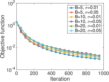
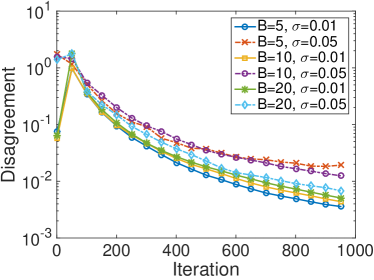
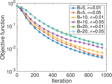
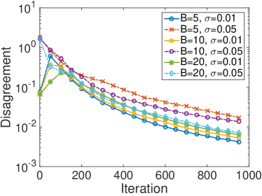
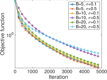
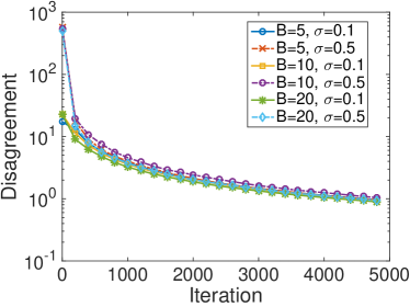
Figure 1: Test on synthetic decentralized least-squares (top), robust least-squares (middle), and logistic regression (bottom) for different levels of delay $B$ and standard deviation in stochastic gradient $\sigma$. Left: objective function $f(z(T))-f^{*}$ versus iteration number $T$, where $f^{*}=f(x^{*})$ is the optimal value. Right: disagreement $\sum_{i=1}^{m}\|y_{i}(T)-z(T)\|^{2}$ versus iteration number $T$.

We also compared the performance of decentralized gradient descent method with and without delay and stochasticity in the gradients. In this test, we synthesized networks and data in the same way as in the decentralized least squares test above. In addition, we plotted the result of $\tau_{i}(t)=0$ for all $i=1,\dots,m$ and $\sigma=0$ is for comparison. These results are shown in the top row of Figure 2, The objective function value (top left) and disagreement (top right) both decay sightly faster when there are no delay and stochastic error as shown in Figure 2, which is within expectations. We further tested the performance when the network size varies. In this experiment, we used four 2D lattice networks, with sizes $m=5^{2},10^{2},15^{2},20^{2}$. The size of $x$ and $A_{i}$ at each node are the same as before. The objective function value (middle left) and disagreement (middle right) both decays, while it appears that network with smaller size decays faster, as shown in Figure 2. To demonstrate effectiveness of asynchronous consensus, we applied EXTRA [34], a state-of-the-arts synchronous decentralized consensus optimization method, to the same data generated in decentralized least squares problem with network size $m=100$ and $\sigma=0$ (no stochastic error in gradients). We draw computing times of these 100 nodes as independent random variables between $[.001,.500]$ms every gradient evaluation. The synchronous algorithm EXTRA needs to wait for the slowest node to finish computation and then start a new iteration, whereas in the asynchronous algorithm (2) the nodes communicate with neighbors every 0.01ms using updates obtained by delayed gradients . We plotted the objective function $f(z(T))-f^{*}$ and disagreement $\sum_{i=1}^{m}\|y_{i}(T)-z(T)\|^{2}$ versus running time in the bottom row of Figure 2, which show that the asynchronous updates can be more time efficient by not waiting for slowest node in each iteration.

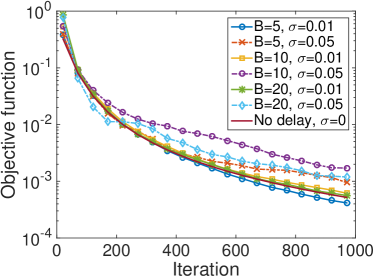
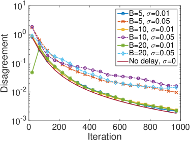
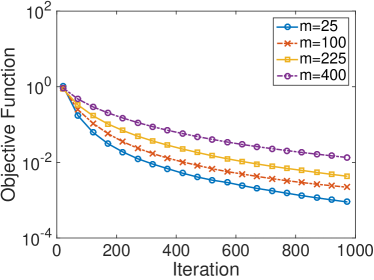
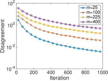
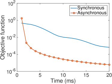
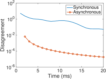
Figure 2: Test on synthetic decentralized least-squares with and without delay/stochasticity (top) and varying network size (bottom). Left: objective function $f(z(T))$ versus iteration number $T$. Right: disagreement $\sum_{i=1}^{m}\|y_{i}(T)-z(T)\|^{2}$ versus iteration number $T$.

4.2 Test on real data

We apply algorithm (2) to seismic tomography where the data is collected and then processed by the nodes (sensors) in a wireless sensor network. In brief, underground seismic activities (such as earthquakes) generate acoustic waves (we use P-wave here) which travel through the materials and are detected by the sensors placed on the ground. An explanatory picture of seismic tomography using a sensor network is shown in Figure 3. After data preprocessing, sensor $i$ obtains a matrix $A_{i}\in\mathbb{R}^{p_{i}\times n}$ and a vector $b_{i}\in\mathbb{R}^{p_{i}}$, and hence an objective $f_{i}(x)=(1/2)\|A_{i}x-b_{i}\|^{2}$ for $i=1,\dots,m$. Here $(A_{i})_{kl}$, the $(k,l)$-th entry of matrix $A_{i}$, is the distance that the wave generated by $k$-th seismic activity travels through pixel $l$, for $k=1,\dots,p_{i}$ ($p_{i}$ is the total number of seismic activities) and $l=1,\dots,n$ ($n$ is the total number of pixels in the image), and $(b_{i})_{k}$, the $k$-th component of $b_{i}$, is the total time that the wave travels from the source of $k$-th seismic activity to the sensor $i$. Then $x_{l}$, the $l$-th component of $x\in\mathbb{R}^{n}$, represents the unknown “slowness” (reciprocal of the velocity of the traveling wave) at that location (pixel) $l$. The sensors then collaboratively solve for the image $x$ that minimizes the sum of their objective functions, under the constraint that only neighbor nodes may communicate during the computation process, since wireless signal transmission can only occur within a limited geographical range. Once $x$ is reconstructed from $\min_{x}f(x)=\sum_{i=1}^{m}f_{i}(x)$, the material (e.g., rock, sand, oil, or magma) at each pixel $l$ can be identified by the value of $x_{l}$.

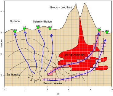
Figure 3: Seismic tomography of an active volcano using wireless sensor network. When there is a seismic activity (e.g., an earthquake) happens underground, its acoustic waves (blue solid curves with arrows) travel to the ground surface and are detected by the sensors (green triangles). Then the sensors communicate wirelessly to reconstruct the entire image, where each square (tan, pink or red) represents a pixel of the image $x\in\mathbb{R}^{n}$.

The first dataset consists of a simple and connected network $G$ with $m=32$ nodes where each node has $3$ neighbors, and $A_{i}\in\mathbb{R}^{p_{i}\times n}$ and $b_{i}\in\mathbb{R}^{p_{i}}$ where the number of seismic events is $p_{i}=512$ and the size of a 2D image $x$ to be reconstructed is $n=64^{2}=4096$. Since the matrix by stacking all $A_{i}$ is still underdetermined, we employ an objective function with Tikhonov regularization as $f_{i}(x)=(1/2)(\|A_{i}x-b_{i}\|^{2}+\mu\|x\|^{2})$ at each node $i$ where $\mu$ is set to $0.1$. Note that more adaptive regularizers of $x$, such as $\ell_{1}$ and total variation (TV) which result in a nonsmooth objective function, will be explored in future research. We apply algorithm (3) with bound $B$ of delays set to $5$, $10$, and $20$ and standard deviation $\sigma$ of stochastic gradient to $0.5$ and $0.05$. We run our algorithm using step size $\alpha(t)=1/(2L+2\eta\sqrt{t})$ with $\eta$ that minimizes the constant of $1/\sqrt{T}$ term in Theorem 3. The objective function $f(z(T))$ and disagreement $\sum_{i=1}^{m}\|y_{i}(T)-z(T)\|^{2}$ versus the iteration number $T$ are plotted in the top row of Figure 4, where convergence of both quantities can be observed.

The second seismic dataset contains a connected network $G$ of size $m=50$ where each node has $3$ neighbors, and matrices $A_{i}\in\mathbb{R}^{p_{i}\times n}$ and $b_{i}\in\mathbb{R}^{p_{i}}$ where $p_{i}=800$ and the size of 3D image $x$ to be reconstructed is $n=32^{3}=32768$. We use the same objective function with Tikhonov regularization as before with $\mu=0.01$. Other parameters are set the same as in the previous test on a 2D seismic image. The settings for $B$ and $\sigma$ remain the same. The objective function $f(z(T))$ and disagreement $\sum_{i=1}^{m}\|y_{i}(T)-z(T)\|^{2}$ versus the iteration number $T$ are plotted in the middle row of Figure 4, where similar convergence behavior can be observed.

The last seismic dataset consists of a connected network $G$ of size $m=10$ where the average node degree is $5$, and matrices $A_{i}\in\mathbb{R}^{p_{i}\times n}$ and $b_{i}\in\mathbb{R}^{p_{i}}$ where $p_{i}=1,816$ and the size of 3D image $x$ to be reconstructed is $n=160\times 200\times 24=768,000$. In this test, we employ objective $f_{i}(x)=(1/2)(\|A_{i}x-b_{i}\|^{2}+\mu\|Dx\|^{2})$ where $\mu=0.1$ and $D$ is the discrete gradient operator. Other parameters are set the same as in the previous two seismic datasets. The bound $B$ of delay is set to $4$, $8$, and $16$, and standard deviation of stochastic gradient $\sigma$ is set to 1e-4 and 5e-4. The objective function $f(z(T))$ and disagreement $\sum_{i=1}^{m}\|y_{i}(T)-z(T)\|^{2}$ versus the iteration number $T$ are plotted in the last row of Figure 4. The reconstructed image is displayed in the right panel of Figure 5. By comparing with the solution obtained by centralized LSQR solver (left), we can see the image is faithfully reconstructed on a decentralized network with delayed stochastic gradients.

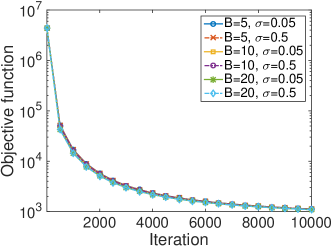
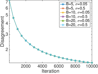
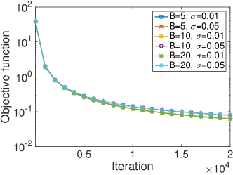
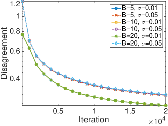
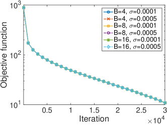
Figure 4: Tests on real seismic image reconstruction problems with $2D$ image with $n=64^{2}$ (top), $3D$ image with $n=32^{3}$ (middle), and $3D$ image with $n=160\times 200\times 24$ (bottom) for different levels of delay $B$ and standard deviation in stochastic gradient $\sigma$. Left: objective function $f(z(T))$ versus iteration number $T$. Optimal value indicates $f^{*}\mathrel{\mathop{\mathchar 58\relax}}=f(x^{*})$. Right: disagreement $\sum_{i=1}^{m}\|y_{i}(T)-z(T)\|^{2}$ versus iteration number $T$.

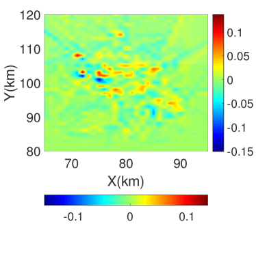
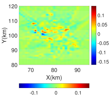
Figure 5: Cross section of a reconstructed 3D seismic image generated by a centralized LSQR solver (left) and decentralized algorithm with delayed stochastic gradient (2) with $B=4$ and $\sigma=10^{-4}$ (right).

5 Concluding Remarks

In this paper, we analyzed the convergence of decentralized delayed stochastic gradient descent method as in (2) for solving the consensus optimization (1). The algorithm takes into consideration that the nodes in the network privately hold parts of the objective function and collaboratively solve for the consensus optimal solution of the total objective while they can only communicate with their immediate neighbors, as well as the delays of gradient information in real-world networks where the nodes cannot be fully synchronized. We show that, as long as the random delays are bounded in expectation and a proper diminishing step size policy is employed, the iterates generated by the decentralized gradient decent method converge to a consensus solution. Convergence rates of both objective and consensus were derived. Numerical results on a number of synthetic and real data were also presented for validation.

Appendix A Proof of Lemma 1

Proof.

It suffices to show that for any fixed $R>0$ and $X=\{x\in\mathbb{R}^{m}\mathrel{\mathop{\mathchar 58\relax}}\|x\|_{\infty}\leq R\}$, there is

$$\|(I-J)\operatorname{\Pi}_{X}(x)\|\leq\|(I-J)x\|$$ (20)

for all $x\in\mathbb{R}^{m}$. Note that for $x=(x_{1},x_{2},\dots,x_{m})^{\top}\in\mathbb{R}^{m}$, there is

$$\|(I-J)x\|^{2}=\sum_{i=1}^{m}(x_{i}-\overline{x})^{2}$$

where $\overline{x}\mathrel{\mathop{\mathchar 58\relax}}=(1/m)\sum_{i=1}^{m}x_{i}$. We only need to show that if all $\{x_{i}\mathrel{\mathop{\mathchar 58\relax}}x_{i}<-R\}$ are projected to $-R$ then $\|(I-J)x\|^{2}$ will reduce. Without loss of generality, suppose $x_{1},\dots,x_{\ell}<-R$ and $x_{\ell+1},\dots,x_{m}\geq-R$, and let denote the means of these two groups by

$$\mu_{1}\mathrel{\mathop{\mathchar 58\relax}}=\frac{1}{\ell}\sum_{i=1}^{\ell}x_{i}<-R\quad\mbox{ and }\quad\mu_{2}\mathrel{\mathop{\mathchar 58\relax}}=\frac{1}{m-\ell}\sum_{i=\ell+1}^{m}x_{i}\geq-R.$$ (21)

Then we have $\overline{x}=(\ell\mu_{1}+(m-\ell)\mu_{2})/m$, and

$$\quad\|(I-J)x\|^{2}$$

$$=\sum_{i=1}^{m}(x_{i}-\overline{x})^{2}=\sum_{i=1}^{m}(x_{i}-\frac{\ell\mu_{1}+(m-\ell)\mu_{2}}{m})^{2}$$

$$=\sum_{i=1}^{\ell}(x_{i}-\frac{\ell\mu_{1}+(m-\ell)\mu_{2}}{m})^{2}+\sum_{i=\ell+1}^{m}(x_{i}-\frac{\ell\mu_{1}+(m-\ell)\mu_{2}}{m})^{2}$$

$$=\sum_{i=1}^{\ell}\left((x_{i}-\mu_{1})+\frac{m-\ell}{m}(\mu_{1}-\mu_{2})\right)^{2}+\sum_{i=\ell+1}^{m}\left((x_{i}-\mu_{2})+\frac{\ell}{m}(\mu_{2}-\mu_{1})\right)^{2}$$ (22)

$$=\sum_{i=1}^{\ell}(x_{i}-\mu_{1})^{2}+2\frac{m-\ell}{m}(\mu_{1}-\mu_{2})\sum_{i=1}^{\ell}(x_{i}-\mu_{1})+\ell\left(\frac{m-\ell}{m}\right)^{2}(\mu_{1}-\mu_{2})^{2}$$

$$\ +\sum_{i=\ell+1}^{m}(x_{i}-\mu_{2})^{2}+2\frac{\ell}{m}(\mu_{2}-\mu_{1})\sum_{i=\ell+1}^{m}(x_{i}-\mu_{2})+(m-\ell)\left(\frac{\ell}{m}\right)^{2}(\mu_{2}-\mu_{1})^{2}$$

After $x_{1},\cdots,x_{\ell}$ are projected to $-R$ (and $x_{\ell+1},\dots,x_{m}$ remain unchanged), their mean is updated from $\mu_{1}$ to $-R$ for all $i=1,\dots,\ell$, and $\mu_{2}-\mu_{1}(\geq 0)$ reduces to $\mu_{2}+R(\geq 0)$. Therefore, the first, third, and sixth terms in the right hand side of (22) are decreased, the second and fifth terms remain zero, and the fourth term remains unchanged. Thus $\|(I-J)x\|$ reduces after projection to $[-R,\infty)^{m}$. A similar argument implies that projecting $\{x_{i}\mathrel{\mathop{\mathchar 58\relax}}x_{i}>R\}$ to $R$ will further reduce $\|(I-J)x\|^{2}$. Therefore projecting $x$ to $X$, i.e., projecting to $[-R,\infty)^{m}$ and then $(-\infty,R]^{m}$, reduces $\|(I-J)x\|^{2}$. ∎

Appendix B Proof of Lemma 2

Proof.

First, we note that

$$\sum_{s=0}^{t-1}\alpha(s)\lambda^{t-1-s}=\alpha(0)\lambda^{t-1}+\alpha(1)\lambda^{t-2}+\sum_{s=2}^{t-1}\alpha(s)\lambda^{t-1-s}$$ (23)

which means that the rate is upper bounded by the last sum on the right side above since the first two tend to $0$ at a linear rate $\lambda\in(0,1)$.

Note that for all $w\in[s-1,s]$ we have $\frac{1}{\sqrt{s}}\leq\frac{1}{\sqrt{w}}$ and $\lambda^{-s}\leq\lambda^{-(w+1)}$ since $\lambda\in(0,1)$, and therefore

$$\alpha(s)\lambda^{t-1-s}=\frac{\lambda^{t-1-s}}{c_{1}+c_{2}\sqrt{s}}\leq\frac{\lambda^{t-1}\lambda^{-s}}{c_{2}\sqrt{s}}\leq\frac{\lambda^{t-1}\lambda^{-(w+1)}}{c_{2}\sqrt{w}}=\frac{\lambda^{t-2-w}}{c_{2}\sqrt{w}}.$$ (24)

This inequality allows us to bound the last term on right hand side of (23) by

$$\sum_{s=2}^{t-1}\alpha(s)\lambda^{t-1-s}\leq\sum_{s=2}^{t-1}\int_{s-1}^{s}\frac{\lambda^{t-2-w}}{c_{2}\sqrt{w}}dw=\int_{1}^{t-1}\frac{\lambda^{t-2-w}}{c_{2}\sqrt{w}}dw=\frac{2\lambda^{t-2}}{c_{2}}I_{t},$$ (25)

where $I_{t}$ is defined by

$$I_{t}\mathrel{\mathop{\mathchar 58\relax}}=\frac{1}{2}\int_{1}^{t-1}\frac{\lambda^{-w}}{\sqrt{w}}dw.$$ (26)

By changing of variable $w=u^{2}$, we obtain $I_{t}=\int_{1}^{\sqrt{t-1}}\lambda^{-u^{2}}du$. Now we have that

$$I_{t}^{2} =\int_{1}^{\sqrt{t-1}}\int_{1}^{\sqrt{t-1}}\lambda^{-(u^{2}+v^{2})}\ dudv=\int_{1}^{\sqrt{t-1}}\int_{1}^{\sqrt{t-1}}e^{-(u^{2}+v^{2})\log\lambda}\ dudv$$

$$\leq\int_{0}^{\sqrt{t}}\int_{0}^{\sqrt{t}}e^{-(u^{2}+v^{2})\log\lambda}\ dudv=2\int_{0}^{\pi/4}\int_{0}^{\sqrt{t}/\cos\theta}e^{-\rho^{2}\log\lambda}\rho\ d\rho d\theta$$ (27)

$$=-\frac{1}{\log\lambda}\int_{0}^{\pi/4}(e^{-t\log\lambda/\cos^{2}(\theta)}-1)\ d\theta<-\frac{1}{\log\lambda}\int_{0}^{\pi/4}e^{-t\log\lambda/\cos^{2}(\theta)}\ d\theta$$

where the third equality comes from changing to a polar system with the substitutions $u=\rho\cos\theta$ and $v=\rho\sin\theta$. Note that $\cos^{-2}(\theta)-(1+4\theta/\pi)\leq 0$ for all $\theta\in[0,\pi/4]$ since $\cos^{-2}(\theta)-1-4\theta/\pi$ is convex with respect to $\theta$ and vanishes at $\theta=0$ and $\theta=\pi/4$. Therefore

$$I_{t}^{2}\leq-\frac{1}{\log\lambda}\int_{0}^{\pi/4}e^{-t\log\lambda(1+4\theta/\pi)}d\theta\leq\frac{\pi\lambda^{-2t}}{4t(\log\lambda)^{2}}.$$ (28)

Hence the sum in (25) is bounded by

$$\sum_{s=2}^{t-1}\alpha(s)\lambda^{t-1-s}\leq\frac{2\lambda^{t-2}}{c_{2}}I_{t}\leq\frac{2\lambda^{t-2}}{c_{2}}\frac{\sqrt{\pi}\lambda^{-t}}{2\sqrt{t}\log(\lambda^{-1})}=\frac{\sqrt{\pi}\lambda^{-2}}{c_{2}\sqrt{t}\log(\lambda^{-1})}$$ (29)

which completes the proof. ∎

Appendix C Proof of Corollary 1

Proof.

According to the update (4) or equivalently (3), we have

$$\operatorname{\mathbb{E}}[\|x(t+1)-x(t)\|] =\operatorname{\mathbb{E}}[\|\operatorname{\Pi}_{\mathcal{X}}[Wx(t)-\alpha(t)g(t-\tau(t))]-x(t)\|]$$

$$\leq\operatorname{\mathbb{E}}[\|(I-W)x(t)+\alpha(t)g(t-\tau(t)))\|]$$ (30)

$$\leq\operatorname{\mathbb{E}}[\|(I-W)x(t)\|]+\alpha(t)\operatorname{\mathbb{E}}[\|g(t-\tau(t)))\|]$$

where we used the facts that $x(t)\in\mathcal{X}$ and that projection $\operatorname{\Pi}_{\mathcal{X}}$ is non-expansive in the first inequality. Note that $WJ=J$ and hence $I-W=(I-W)(I-J)$, we have

$$\operatorname{\mathbb{E}}[\|(I-W)x(t)\|]=\operatorname{\mathbb{E}}[\|(I-W)(I-J)x(t)\|]\leq\operatorname{\mathbb{E}}[\|(I-J)x(t)\|]\leq\frac{\sqrt{\pi m}G\lambda^{-2}}{\eta\sqrt{t}\log(\lambda^{-1})}$$

where we used the fact that $\|I-W\|\leq 1$ in the first inequality and applied Theorem 1 to obtain the second inequality.

Furthermore, we have by the definition of $\alpha(t)$ that

$$\|\alpha(t)g(t-\tau(t))\|\leq\sqrt{m}\alpha(t)G=\frac{\sqrt{m}G}{2(L+\eta\sqrt{t})}\leq\frac{\sqrt{m}G}{2\eta\sqrt{t}}.$$ (31)

Applying the two inequalities above to (C) yields (12). ∎

Appendix D Proof of Corollary 2

Proof.

We first define $\bar{\tau}(t)\mathrel{\mathop{\mathchar 58\relax}}=\max\{\tau_{i}(t)\mathrel{\mathop{\mathchar 58\relax}}1\leq i\leq m\}$. Then there is $\operatorname{\mathbb{E}}[|\bar{\tau}(t)|^{2}]\leq\operatorname{\mathbb{E}}[\sum_{i=1}^{m}|\tau_{i}(t)|^{2}]\leq mB^{2}$. Without loss of generality, we assume that $0\leq\bar{\tau}(t)\leq t-2$ for every given $t$, i.e., we consider the convergence rate when every node has successfully computed their own gradient at least twice. Then we obtain that

$$\quad\,\operatorname{\mathbb{E}}[\|x(t)-x(t-\tau(t))\|]$$

$$\leq\operatorname{\mathbb{E}}\mathinner{\biggl{[}\sum_{s=1}^{\bar{\tau}(t)}\|x(t-s+1)-x(t-s)\|\biggr{]}}\leq C\operatorname{\mathbb{E}}\mathinner{\biggl{[}\sum_{s=1}^{\bar{\tau}(t)}\frac{1}{\sqrt{t-s}}\biggr{]}}$$

$$=C\operatorname{\mathbb{E}}\mathinner{\biggl{[}\sum_{s=t-\bar{\tau}(t)}^{t-1}\frac{1}{\sqrt{s}}\biggr{]}}\leq C\operatorname{\mathbb{E}}\mathinner{\biggl{[}\int_{t-\bar{\tau}(t)-1}^{t-1}\frac{1}{\sqrt{s}}ds\biggr{]}}$$ (32)

$$=2C\operatorname{\mathbb{E}}\mathinner{\left[\sqrt{t-1}-\sqrt{t-\bar{\tau}(t)-1}\right]}\leq 2C\operatorname{\mathbb{E}}\mathinner{\biggl{[}\frac{\bar{\tau}(t)}{\sqrt{t-1}+\sqrt{t-\bar{\tau}(t)-1}}\biggr{]}}$$

$$\leq C\operatorname{\mathbb{E}}\mathinner{\biggl{[}\frac{\bar{\tau}(t)}{\sqrt{t-\bar{\tau}(t)-1}}\biggr{]}}$$

where we used triangle inequality to obtain the first inequality, applied Corollary 1 to obtain the second inequality, and used the fact that $\bar{\tau}(t)\geq 0$ to obtain the last inequality above. Note that there is

$$\operatorname{\mathbb{E}}\mathinner{\left[\frac{\bar{\tau}(t)}{\sqrt{t-\bar{\tau}(t)-1}}\right]} =\sum_{s=0}^{\lfloor t/2\rfloor-1}\frac{s}{\sqrt{t-s-1}}\operatorname{\mathrm{P}}(\bar{\tau}(t)=s)+\sum_{s=\lfloor t/2\rfloor}^{t-2}\frac{s}{\sqrt{t-s-1}}\operatorname{\mathrm{P}}(\bar{\tau}(t)=s)$$

$$\leq\frac{\sqrt{2}}{\sqrt{t}}\sum_{s<t/2}s\operatorname{\mathrm{P}}(\bar{\tau}(t)=s)+(t-2)\sum_{s\geq t/2}\operatorname{\mathrm{P}}(\bar{\tau}(t)=s)$$ (33)

$$\leq\frac{\sqrt{2m}B}{\sqrt{t}}+\frac{4mB^{2}(t-2)}{t^{2}}\leq\frac{\sqrt{2m}B}{\sqrt{t}}+\frac{4mB^{2}}{t}=O\mathinner{\left(\frac{1}{\sqrt{t}}\right)}$$

where we used the fact that $\sqrt{t-s-1}\geq\sqrt{t/2}$ if $0\leq s\leq\lfloor t/2\rfloor-1$ and $s/\sqrt{t-s-1}\leq t-2$ if $\lfloor t/2\rfloor\leq s\leq t-2$ to obtain the first inequality, and $\sum_{s<t/2}s\operatorname{\mathrm{P}}(\bar{\tau}(t)=s)\leq\operatorname{\mathbb{E}}[\bar{\tau}(t)]\leq\sqrt{\operatorname{\mathbb{E}}[\bar{\tau}(t)^{2}]}=\sqrt{m}B$ and $\sum_{s\geq t/2}\operatorname{\mathrm{P}}(\bar{\tau}(t)=s)=\operatorname{\mathrm{P}}(\bar{\tau}(t)\geq t/2)\leq(4/t^{2})\operatorname{\mathbb{E}}[\bar{\tau}(t)^{2}]\leq 4mB^{2}/t^{2}$ (by Chebyshev’s inequality) in the second inequality. In particular, it is easy to verify that, when $t\geq 8mB^{2}$, there is $\sqrt{2m}B/\sqrt{t}\geq 4mB^{2}/t$ and hence $\operatorname{\mathbb{E}}\mathinner{\Bigl{[}\frac{\bar{\tau}(t)}{\sqrt{t-\bar{\tau}(t)-1}}\Bigr{]}}\leq\frac{2\sqrt{2m}B}{\sqrt{t}}$. Combining (32) and (33) completes the proof. ∎

Appendix E Proof of Lemma 3

Proof.

By Cauchy-Schwarz inequality, we have that

$$\quad\,\sum_{t=1}^{T}\langle\nabla f(x(t))-\nabla f(x(t-\tau(t))),x(t+1)-x^{*}\rangle$$

$$\leq\sum_{t=1}^{T}\|\nabla f(x(t))-\nabla f(x(t-\tau(t))\|\|x(t+1)-x^{*}\|$$

Note that $\|x(t+1)-x^{*}\|^{2}=\sum_{i=1}^{m}\|x_{i}(t+1)-x^{*}\|^{2}\leq mn(2R)^{2}$ due to the bound of $X=\{x\in\mathbb{R}^{n}\mathrel{\mathop{\mathchar 58\relax}}\|x\|_{\infty}\leq R\}$, and $\|\nabla f(x(t))-\nabla f(x(t-\tau(t))\|^{2}=\sum_{i=1}^{m}\|\nabla f_{i}(x_{i}(t))-\nabla f_{i}(x_{i}(t-\tau(t))\|^{2}\leq\sum_{i=1}^{m}L_{i}\|x_{i}(t)-x_{i}(t-\tau(t))\|^{2}\leq L\|x(t)-x(t-\tau(t))\|^{2}\leq 2\sqrt{2m}CB/\sqrt{t}$ due to Corollary 2. Therefore, we obtain

$$\sum_{t=1}^{T}\langle\nabla f(x(t))-\nabla f(x(t-\tau(t))),x(t+1)-x^{*}\rangle\leq 8\sqrt{2nLT}mRCB$$

by using the fact that $\sum_{t=1}^{T}1/\sqrt{t}\leq 2\sqrt{T}$. This completes the proof. ∎

Appendix F Proof of Theorem 2

Proof.

We first note that there is

$$\qquad f(x(t+1))-f(x^{*})=\sum_{i=1}^{m}\left(f_{i}(x_{i}(t+1))-f_{i}(x^{*})\right)$$

$$=\ \sum_{i=1}^{m}\left[f_{i}(x_{i}(t+1))-f_{i}(x_{i}(t))+f_{i}(x_{i}(t))-f_{i}(x^{*})\right]$$

$$\leq\ \sum_{i=1}^{m}\left[\left\langle\nabla f_{i}(x_{i}(t)),x_{i}(t+1)-x_{i}(t)\right\rangle+\frac{L_{i}}{2}\|x_{i}(t+1)-x_{i}(t)\|^{2}\right.$$ (34)

$$\qquad\qquad\left.+\left\langle\nabla f_{i}(x_{i}(t)),x_{i}(t)-x^{*}\right\rangle\right]$$

$$\leq\ \sum_{i=1}^{m}\left[\left\langle\nabla f_{i}(x_{i}(t)),x_{i}(t+1)-x^{*}\right\rangle+\frac{L_{i}}{2}\|x_{i}(t+1)-x_{i}(t)\|^{2}\right]$$

$$\leq\ \left\langle\nabla f(x(t)),x(t+1)-x^{*}\right\rangle+\frac{L}{2}\|x(t+1)-x(t)\|^{2}$$

$$\leq\ \left\langle g(t-\tau(t)),x(t+1)-x^{*}\right\rangle+\left\langle\nabla f(x(t))-g(t-\tau(t)),x(t+1)-x^{*}\right\rangle$$

$$\qquad\qquad+\frac{L}{2}\|x(t+1)-x(t)\|^{2}$$

where we used the $L_{i}$-Lipschitz continuity of $\nabla f_{i}$ and convexity of $f_{i}$ to obtain the first inequality. Note that $x(t+1)$ is obtained by (4) as

$$x(t+1)= \mathop{\rm argmin}_{x\in\mathcal{X}}\left\{\langle g(t-\tau(t)),x\rangle+\frac{1}{2\alpha(t)}\|x-Wx(t)\|^{2}\right\}$$ (35)

$$= \mathop{\rm argmin}_{x\in\mathcal{X}}\left\{\left\langle g(t-\tau(t))+\frac{1}{\alpha(t)}(I-W)x(t),x\right\rangle+\frac{1}{2\alpha(t)}\|x-x(t)\|^{2}\right\}$$

Therefore, the optimality of $x(t+1)$ in (4) and strong convexity of the objective function in (4) imply that

$$\left\langle g(t-\tau(t)),x(t+1)-x^{*}\right\rangle$$

$$\leq -\frac{1}{\alpha(t)}\left\langle(I-W)x(t),x(t+1)-x^{*}\right\rangle$$ (36)

$$+\frac{1}{2\alpha(t)}\left[\|x^{*}-x(t)\|^{2}-\|x(t+1)-x(t)\|^{2}-\|x^{*}-x(t+1)\|^{2}\right].$$

Furthermore, we note that $\mathbf{1}\in\mathrm{Null}(I-W)$ and $x^{*}$ is consensual, hence we have

$$\ -\frac{1}{\alpha(t)}\langle(I-W)x(t),x(t+1)-x^{*}\rangle$$

$$= \ -\frac{1}{\alpha(t)}\langle(I-W)(x(t)-x^{*}),x(t+1)-x^{*}\rangle$$

$$= \ \frac{1}{2\alpha(t)}\left(\|x(t)-x(t+1)\|_{I-W}^{2}-\|x(t)-x^{*}\|_{I-W}^{2}-\|x(t+1)-x^{*}\|_{I-W}^{2}\right)$$ (37)

$$\leq \ \frac{1}{4\alpha(t)}\|x(t)-x(t+1)\|_{I-W}^{2}$$

where we have used the fact that

$$\|x(t)-x(t+1)\|_{I-W}^{2}\leq 2(\|x(t)-x^{*}\|_{I-W}^{2}+\|x(t+1)-x^{*}\|_{I-W}^{2})$$

to obtain the inequality above. We also have that

$$\|x(t)-x(t+1)\|_{I-W}^{2}\leq\|x(t)-x(t+1)\|^{2}$$

with which we can further bound (F) as

$$-\frac{1}{\alpha(t)}\langle(I-W)x(t),x(t+1)-x^{*}\rangle\leq\frac{1}{4\alpha(t)}\|x(t)-x(t+1)\|^{2}.$$

Now applying the inequality above and (F) to (F), and taking sum of $t$ from $1$ to $T$, we get

$$\sum_{t=1}^{T}f(x(t+1))-Tf(x^{*}) \leq\ \sum_{t=1}^{T}\frac{1}{2\alpha(t)}\left(\|x(t)-x^{*}\|^{2}-\|x(t+1)-x^{*}\|^{2}\right)$$

$$\quad+\sum_{t=1}^{T}\left(\frac{L}{2}-\frac{1}{4\alpha(t)}\right)\|x(t)-x(t+1)\|^{2}$$ (38)

$$\quad+\sum_{t=1}^{T}\left\langle\nabla f(x(t))-g(t-\tau(t)),x(t+1)-x^{*}\right\rangle.$$

Note that the running average $y(T)=(1/T)\sum_{t=1}^{T}x(t+1)$ satisfies $f(y(T))\leq(1/T)\sum_{t=1}^{T}f(x(t+1))$ due to the convexity of all $f_{i}$. Therefore, together with (F) and the definition of $\alpha(t)$, we have

$$\ T[f(y(T))-f(x^{*})]$$

$$\leq \ \sum_{t=1}^{T}\left[\frac{1}{2\alpha(t)}\left(\|x(t)-x^{*}\|^{2}-\|x(t+1)-x^{*}\|^{2}\right)-\frac{\eta\sqrt{t}}{2}\|x(t)-x(t+1)\|^{2}\right]$$ (39)

$$\ +\sum_{t=1}^{T}\left\langle\nabla f(x(t))-g(x(t-\tau(t))),x(t+1)-x^{*}\right\rangle.$$

Now, by taking expectation on both sides of (F), we obtain

$$T\operatorname{\mathbb{E}}[f(y(T))-f(x^{*})]\leq \ \sum_{t=1}^{T}\left[\frac{1}{2\alpha(t)}\left(e(t)-e(t+1)\right)-\frac{\eta\sqrt{t}}{2}\operatorname{\mathbb{E}}[\|x(t)-x(t+1)\|^{2}]\right]$$

$$+8\sqrt{2nLT}mRCB$$ (40)

$$+\sum_{t=1}^{T}\operatorname{\mathbb{E}}\left\langle\nabla f(x(t-\tau(t)))-g(t-\tau(t)),x(t+1)-x^{*}\right\rangle$$

where we denoted $e(t)\mathrel{\mathop{\mathchar 58\relax}}=\operatorname{\mathbb{E}}[\|x(t)-x^{*}\|^{2}]$ for notation simplicity.

Now we work on the last sum of inner products on the right side of (F). First we observe that

$$\ \operatorname{\mathbb{E}}\left\langle\nabla f(x(t-\tau(t)))-g(t-\tau(t)),x(t+1)-x^{*}\right\rangle$$

$$= \ \operatorname{\mathbb{E}}\left\langle\nabla f(x(t-\tau(t)))-g(t-\tau(t)),x(t-\tau(t))-x^{*}\right\rangle$$ (41)

$$\qquad+\operatorname{\mathbb{E}}\left\langle\nabla f(x(t-\tau(t)))-g(t-\tau(t)),x(t+1)-x(t-\tau(t))\right\rangle.$$

Note that $g_{i}(t-\tau_{i}(t))$ is the stochastic gradient of node $i$ evaluated at iteration $t-\tau_{i}(t)$, and the stochastic error $g_{i}(t-\tau_{i}(t))-\nabla f_{i}(x_{i}(t-\tau_{i}(t)))$ is independent of $x_{i}(t-\tau_{i}(t))$. Therefore, we have

$$\quad\,\operatorname{\mathbb{E}}\left\langle\nabla f(x(t-\tau(t)))-g(t-\tau(t)),x(t-\tau(t))-x^{*}\right\rangle$$ (42)

$$=\sum_{i=1}^{m}\operatorname{\mathbb{E}}\left\langle\nabla f_{i}(x_{i}(t-\tau_{i}(t)))-g_{i}(t-\tau_{i}(t)),x_{i}(t-\tau_{i}(t))-x^{*}\right\rangle=0,$$

since the stochastic gradients are unbiased. Furthermore, by Young’s inequality, we have

$$\ \operatorname{\mathbb{E}}\left\langle\nabla f(x(t-\tau(t)))-g(t-\tau(t)),x(t+1)-x(t-\tau(t))\right\rangle$$

$$\leq \ \frac{2}{\eta\sqrt{t}}\operatorname{\mathbb{E}}[\|\nabla f(x(t-\tau(t)))-g(t-\tau(t))\|^{2}]+\frac{\eta\sqrt{t}}{2}\operatorname{\mathbb{E}}[\|x(t+1)-x(t)\|^{2}]$$ (43)

$$\leq \ \frac{2m\sigma^{2}}{\eta\sqrt{t}}+\frac{\eta\sqrt{t}}{2}\operatorname{\mathbb{E}}[\|x(t+1)-x(t)\|^{2}]$$

where we used the fact that $\operatorname{\mathbb{E}}[\|\nabla f(x(t-\tau(t)))-g(t-\tau(t))\|^{2}]\leq m\sigma^{2}$ for all $t$. Now applying (F), (42) and (F) in (F), we have

$$\qquad T\operatorname{\mathbb{E}}\left[f(y(T))-f(x^{*})\right]$$

$$\ \leq\sum_{t=1}^{T}\frac{1}{2\alpha(t)}\left(e(t)-e(t+1)\right)+8\sqrt{2nLT}mRCB+\sum_{t=1}^{T}\frac{2m\sigma^{2}}{\eta\sqrt{t}}$$ (44)

$$\ \leq\frac{e(1)}{2\alpha(1)}+\sum_{t=2}^{T}\frac{e(t)}{2}\left(\frac{1}{\alpha(t)}-\frac{1}{\alpha(t-1)}\right)+8\sqrt{2nLT}mRCB+\sum_{t=1}^{T}\frac{2m\sigma^{2}}{\eta\sqrt{t}}$$

where we note that $\alpha(t)$ is nonincreasing, and hence $\frac{1}{\alpha(t)}-\frac{1}{\alpha(t-1)}\geq 0$ and

$$\sum_{t=2}^{T}\frac{e(t)}{2}\left(\frac{1}{\alpha(t)}-\frac{1}{\alpha(t-1)}\right)\leq\frac{\mathcal{D}_{\mathcal{X}}^{2}}{2}\sum_{t=2}^{T}\left(\frac{1}{\alpha(t)}-\frac{1}{\alpha(t-1)}\right)=\frac{\mathcal{D}_{\mathcal{X}}^{2}}{2}\mathinner{\left(\frac{1}{\alpha(T)}-\frac{1}{\alpha(1)}\right)}$$

where we used the fact that $e(t)=\operatorname{\mathbb{E}}[\|x(t)-x^{*}\|^{2}]\leq\mathcal{D}_{\mathcal{X}}^{2}\mathrel{\mathop{\mathchar 58\relax}}=4mnR^{2}$ for all $t$. Plugging this into (F), dividing both sides by $T$, and using the fact that $\sum_{t=1}^{T}1/\sqrt{t}\leq 2\sqrt{T}$, we obtain (15). This completes the proof. ∎

References

- [1] A. Agarwal and J. C. Duchi. Distributed delayed stochastic optimization. In Advances in Neural Information Processing Systems, pages 873–881, 2011.
- [2] T. C. Aysal, M. E. Yildiz, A. D. Sarwate, and A. Scaglione. Broadcast gossip algorithms for consensus. Signal Processing, IEEE Transactions on, 57(7):2748–2761, 2009.
- [3] S. Boyd, N. Parikh, E. Chu, B. Peleato, and J. Eckstein. Distributed optimization and statistical learning via the alternating direction method of multipliers. Foundations and Trends® in Machine Learning, 3(1):1–122, 2011.
- [4] V. Cevher, S. Becker, and M. Schmidt. Convex optimization for big data: Scalable, randomized, and parallel algorithms for big data analytics. Signal Processing Magazine, IEEE, 31(5):32–43, 2014.
- [5] T.-H. Chang, M. Hong, W.-C. Liao, and X. Wang. Asynchronous distributed admm for large-scale optimization part i: Algorithm and linear convergence analysis. IEEE Transactions on Signal Processing, 64(12):3118–3130, 2016.
- [6] T.-H. Chang, M. Hong, and X. Wang. Multi-agent distributed optimization via inexact consensus admm. Signal Processing, IEEE Transactions on, 63(2):482–497, 2015.
- [7] T.-H. Chang, W.-C. Liao, M. Hong, and X. Wang. Asynchronous distributed admm for large-scale optimization part ii: Linear convergence analysis and numerical performance. IEEE Transactions on Signal Processing, 64(12):3131–3144, 2016.
- [8] J. C. Duchi, A. Agarwal, and M. J. Wainwright. Dual averaging for distributed optimization: convergence analysis and network scaling. Automatic control, IEEE Transactions on, 57(3):592–606, 2012.
- [9] H. R. Feyzmahdavian, A. Aytekin, and M. Johansson. A delayed proximal gradient method with linear convergence rate. In Machine Learning for Signal Processing (MLSP), 2014 IEEE International Workshop on, pages 1–6. IEEE, 2014.
- [10] P. A. Forero, A. Cano, and G. B. Giannakis. Consensus-based distributed support vector machines. The Journal of Machine Learning Research, 11:1663–1707, 2010.
- [11] L. Gan, U. Topcu, and S. H. Low. Optimal decentralized protocol for electric vehicle charging. Power Systems, IEEE Transactions on, 28(2):940–951, 2013.
- [12] F. Iutzeler, P. Bianchi, P. Ciblat, and W. Hachem. Explicit convergence rate of a distributed alternating direction method of multipliers. IEEE Transactions on Automatic Control, 61(4):892–904, 2016.
- [13] F. Iutzeler, P. Ciblat, W. Hachem, and J. Jakubowicz. New broadcast based distributed averaging algorithm over wireless sensor networks. In Acoustics, Speech and Signal Processing (ICASSP), 2012 IEEE International Conference on, pages 3117–3120. IEEE, 2012.
- [14] D. Jakovetic, J. M. Moura, and J. Xavier. Linear convergence rate of a class of distributed augmented lagrangian algorithms. Automatic Control, IEEE Transactions on, 60(4):922–936, 2015.
- [15] D. Jakovetic, J. Xavier, and J. M. Moura. Fast distributed gradient methods. Automatic Control, IEEE Transactions on, 59(5):1131–1146, 2014.
- [16] T. Kraska, A. Talwalkar, J. C. Duchi, R. Griffith, M. J. Franklin, and M. I. Jordan. Mlbase: A distributed machine-learning system. In CIDR, volume 1, pages 2–1, 2013.
- [17] J. Li, G. Chen, Z. Dong, and Z. Wu. Distributed mirror descent method for multi-agent optimization with delay. Neurocomputing, 2015.
- [18] M. Li, D. G. Andersen, and A. Smola. Distributed delayed proximal gradient methods. In NIPS Workshop on Optimization for Machine Learning, 2013.
- [19] M. Li, D. G. Andersen, A. J. Smola, and K. Yu. Communication efficient distributed machine learning with the parameter server. In Advances in Neural Information Processing Systems, pages 19–27, 2014.
- [20] J. Liu, S. J. Wright, C. Ré, V. Bittorf, and S. Sridhar. An asynchronous parallel stochastic coordinate descent algorithm. The Journal of Machine Learning Research, 16(1):285–322, 2015.
- [21] C.-H. Lo and N. Ansari. Decentralized controls and communications for autonomous distribution networks in smart grid. Smart Grid, IEEE Transactions on, 4(1):66–77, 2013.
- [22] L. Lovász. Random walks on graphs: A survey. Combinatorics, Paul Erdős is eighty, 2(1):1–46, 1993.
- [23] A. Makhdoumi and A. Ozdaglar. Convergence rate of distributed admm over networks. IEEE Transactions on Automatic Control, 2017.
- [24] A. Mokhtari and A. Ribeiro. Decentralized double stochastic averaging gradient. In Signals, Systems and Computers, 2015 49th Asilomar Conference on, pages 406–410. IEEE, 2015.
- [25] A. Nedic and A. Olshevsky. Distributed optimization over time-varying directed graphs. Automatic Control, IEEE Transactions on, 60(3):601–615, 2015.
- [26] A. Nedić and A. Olshevsky. Stochastic gradient-push for strongly convex functions on time-varying directed graphs. IEEE Transactions on Automatic Control, 61(12):3936–3947, 2016.
- [27] A. Nedic and A. Ozdaglar. Distributed subgradient methods for multi-agent optimization. Automatic Control, IEEE Transactions on, 54(1):48–61, 2009.
- [28] Y. Nesterov. A method for unconstrained convex minimization problem with the rate of convergence o (1/k2). Technical Report 3, Doklady AN SSSR, 1983.
- [29] R. Olfati-Saber and R. M. Murray. Consensus problems in networks of agents with switching topology and time-delays. Automatic Control, IEEE Transactions on, 49(9):1520–1533, 2004.
- [30] M. Rabbat and R. Nowak. Distributed optimization in sensor networks. In Proceedings of the 3rd international symposium on Information processing in sensor networks, pages 20–27. ACM, 2004.
- [31] A. Sayed. Adaptation, learning, and optimization over networks. Foundations and Trends® in Machine Learning, 7(4-5):311–801, 2014.
- [32] A. H. Sayed, S.-Y. Tu, and J. Chen. Online learning and adaptation over networks: More information is not necessarily better. In Information Theory and Applications Workshop (ITA), 2013, pages 1–8. IEEE, 2013.
- [33] O. Shamir and N. Srebro. Distributed stochastic optimization and learning. In Communication, Control, and Computing (Allerton), 2014 52nd Annual Allerton Conference on, pages 850–857. IEEE, 2014.
- [34] W. Shi, Q. Ling, G. Wu, and W. Yin. Extra: An exact first-order algorithm for decentralized consensus optimization. SIAM Journal on Optimization, 25(2):944–966, 2015.
- [35] W. Shi, Q. Ling, K. Yuan, G. Wu, and W. Yin. On the linear convergence of the admm in decentralized consensus optimization. Signal Processing, IEEE Transactions on, 62(7):1750–1761, 2014.
- [36] W.-Z. Song, R. Huang, M. Xu, A. Ma, B. Shirazi, and R. LaHusen. Air-dropped sensor network for real-time high-fidelity volcano monitoring. In Proceedings of the 7th international conference on Mobile systems, applications, and services, pages 305–318. ACM, 2009.
- [37] S. Sra, A. W. Yu, M. Li, and A. J. Smola. Adadelay: Delay adaptive distributed stochastic convex optimization. In Proceedings of the 19th International Conference on Artificial Intelligence and Statistics, volume 51, pages 957–965, 2016.
- [38] Y.-P. Tian and C.-L. Liu. Consensus of multi-agent systems with diverse input and communication delays. Automatic Control, IEEE Transactions on, 53(9):2122–2128, 2008.
- [39] P. Tseng. On accelerated proximal gradient methods for convex-concave optimization. submitted to SIAM Journal on Optimization, 2008.
- [40] J. N. Tsitsiklis. Problems in decentralized decision making and computation. Technical report, DTIC Document, 1984.
- [41] H. Wang, X. Liao, T. Huang, and C. Li. Cooperative distributed optimization in multiagent networks with delays. Systems, Man, and Cybernetics: Systems, IEEE Transactions on, 45(2):363–369, 2015.
- [42] E. Wei and A. Ozdaglar. On the o(1/k) convergence of asynchronous distributed alternating direction method of multipliers. In Global Conference on Signal and Information Processing (GlobalSIP), 2013 IEEE, pages 551–554. IEEE, 2013.
- [43] T. Wu, K. Yuan, Q. Ling, W. Yin, and A. H. Sayed. Decentralized consensus optimization with asynchrony and delays. In Proceedings of IEEE Asilomar Conference on Signals, Systems, and Computers, 2016.
- [44] L. Xiao and S. Boyd. Fast linear iterations for distributed averaging. Systems & Control Letters, 53(1):65–78, 2004.
- [45] D. Yuan, D. W. Ho, and S. Xu. Regularized primal-dual subgradient method for distributed constrained optimization. IEEE Transactions on Cybernetics, 2015.
- [46] K. Yuan, Q. Ling, and W. Yin. On the convergence of decentralized gradient descent. SIAM Journal on Optimization, 26(3):1835–1854, 2016.
- [47] R. Zhang and J. Kwok. Asynchronous distributed admm for consensus optimization. In Proceedings of the 31st International Conference on Machine Learning (ICML-14), pages 1701–1709, 2014.
- [48] W. Zhang, S. Gupta, X. Lian, and J. Liu. Staleness-aware async-sgd for distributed deep learning. In Proceedings of the 25th International Joint Conference on Artificial Intelligence, pages 2350–2356, 2016.
- [49] L. Zhao, W.-Z. Song, L. Shi, and X. Ye. Decentralised seismic tomography computing in cyber-physical sensor systems. Cyber-Physical Systems, pages 1–22, 2015.
- [50] L. Zhao, W.-Z. Song, and X. Ye. Fast decentralized gradient descent method and applications to in-situ seismic tomography. In Big Data (Big Data), 2015 IEEE International Conference on, pages 908–917. IEEE, 2015.