Quantum Rotor Theory of Systems of Spin-2 Bosons
Abstract
We consider quantum phases of tightly-confined spin-2 bosons in an external field under the presence of rotationally-invariant interactions. Generalizing previous treatments, we show how this system can be mapped onto a quantum rotor model. Within the rotor framework, low-energy excitations about fragmented states, which cannot be accessed within standard Bogoliubov theory, can be obtained. In the spatially extended system in the thermodynamic limit there exists a mean-field ground state degeneracy between a family of nematic states for appropriate interaction parameters. It has been established that quantum fluctuations lift this degeneracy through the mechanism of order-by-disorder and select either a uniaxial or square-biaxial ground state. On the other hand, in the full quantum treatment of the analogous single-spatial mode problem with finite particle number it is known that, due to symmetry restoring fluctuations, there is a unique ground state across the entire nematic region of the phase diagram. Within the established rotor framework we investigate the possible quantum phases under the presence of a quadratic Zeeman field, a problem which has previously received little attention. By investigating wave function overlaps we do not find any signatures of the order-by-disorder phenomenon which is present in the continuum case. Motivated by this we consider an alternative external potential which breaks less symmetry than the quadratic Zeeman field. For this case we do find the phenomenon of order-by-disorder in the fully quantum system. This is established within the rotor framework and with exact diagonalization.
pacs:
03.75.Hh, 05.30.Jp, 03.75.Kk, 03.75.MnI Introduction
Ultracold spinor atoms provide simple and experimentally well-controlled many-body systems with internal degrees of freedom. The simplest case is that of a spin-1 gas. The atomic spin-1 species and have been the subject of numerous experiments (see for example the reviews in Stamper-Kurn and Ueda (2013); Kawaguchi and Ueda (2012) and references therein), prompting detailed theoretical investigation of the exact spectra for tightly confined spin-1 atoms Law et al. (1998); Ho and Yip (2000); Koashi and Ueda (2000); Mueller et al. (2006); Barnett et al. (2010, 2011); Lamacraft (2010) as well as their mean-field properties in the thermodynamic limit Ho (1998); Ohmi and Machida (1998). The higher spin-2 hyperfine multiplet of was found to be stable and amenable to experimental manipulation Chang et al. (2004); Kuwamoto et al. (2004); Schmaljohann et al. (2004); Burke et al. (1997), prompting the development of a number of spin-2 exact and mean-field theoretical results Ciobanu et al. (2000); Koashi and Ueda (2000); Ueda and Koashi (2002); Song et al. (2007); Turner et al. (2007). In particular, Gross-Pitaevskii mean field theory has been used to describe spin-2 condensates under linear and quadratic Zeeman fields Saito and Ueda (2005); Uchino et al. (2010). Exact quantum results have also been found for spin-2 systems under tight spatial confinement under no external fields, which can be simply extended to results with a linear Zeeman field by a gauge transformation Ueda and Koashi (2002); Koashi and Ueda (2000). The case of the quantum states of tightly confined bosons under the presence of a quadratic Zeeman field, however, has remained less well understood.
Spinor condensates also provide a convenient platform with which to study the phenomenon of order-by-disorder Villain et al. (1980); Henley (1987, 1989), or the selection of a particular mean-field ground state from a set of accidentally degenerate ones due to fluctuations. This subject has traditionally been of importance in elucidating the ground-state structure of frustrated magnetic systems but has also been investigated as a relevant mechanism in several cold-atom systems Wessel and Troyer (2005); Song et al. (2007); Turner et al. (2007); Wu (2008); Zhao and Liu (2008); Barnett et al. (2012); You et al. (2012); Zheng et al. (2013); Sun and Vekua (2014); Payrits and Barnett (2014). These offer the possibility of experimentally realizing a phenomenon whose observation is still contentious in magnetic systems Ross et al. (2014); Petit et al. (2014). In spin-2 systems, order by disorder has been predicted to determine the ground state in the absence of a quadratic Zeeman field for species with scattering lengths within a certain range, termed the nematic region. Furthermore, the mechanism has been predicted to introduce a first-order phase transition between two parts of the nematic region in which fluctuations select different members of the accidentally degenerate family Song et al. (2007); Turner et al. (2007).
One of the goals of the present article is to present analytical results for tightly confined spin-2 atoms in the presence of a quadratic Zeeman field. The results are obtained by utilizing an exact mapping of the interacting many-body system Hamiltonian to a 5-dimensional quantum rotor Hamiltonian, i.e., that of a single particle moving on the 4-sphere. Similar mappings have previously been employed to study the double-well problem Anglin et al. (2001), dipolar condensates Armaitis et al. (2013) and particularly the analogous tightly bound spin-1 problem Barnett et al. (2010, 2011); Jing et al. (2011); Buchmann et al. (2013).
One of the main perceived advantages of the rotor methodology is that it allows one to treat excitations about fragmented states Penrose and Onsager (1956); Nozières, P. and Saint James, D. (1982). Applying the Penrose-Onsager criterion for Bose-Einstein condensation, fragmented condensates are defined as those whose reduced single-particle density matrix has more than one extensive eigenvalue. When there are exactly two such eigenvalues, one may envision the state as a condensate of particle pairs. One encounters such a case in the spin-2 problem in the presence of a large negative quadratic Zeeman field. Such a state cannot be approximated by a coherent state, invalidating the use of Bogoliubov theory, typically the first line of attack in calculating excitation spectra about non-fragmented condensates. The rotor mapping, on the other hand, suffers no pathologies in the fragmented case and provides simple analytical expressions for the excitation spectra.
Previous results by Koashi and Ueda Koashi and Ueda (2000); Ueda and Koashi (2002) indicate that the exact quantum results in the absence of a quadratic Zeeman field do not mirror the continuous accidental degeneracy of the mean-field analysis. Rather, the ground state is non-degenerate and the same across the entire nematic region and no traces of the order-by-disorder induced phase transition are manifest. One may hope that the signature of the transition could nevertheless be observed in the magnetic response to the quadratic Zeeman field, which serves to classically orient the nematic order parameter. In the present article we find through an evaluation of the wave function overlaps obtained through the rotor mapping, that such a signature is nevertheless not present.
Motivated by this, we have applied the rotor mapping to the analysis of an alternative potential that does not fully break the mean-field degeneracy, noting that a large class of quadratic potentials can be experimentally obtained with external microwave fields. Using the rotor framework we show that including quantum corrections select a unique ground state. Furthermore, this selection is explicitly demonstrated through an exact diagonalization numerical approach involving a modest number of atoms. Importantly, we find that the overlap of the obtained ground states with any mean-field state tends to zero with increasing particle number, a stark departure from the standard mean-field states obtained in the continuum. On the other hand, the ordering is apparent in the spin-component occupation numbers, which can be readily experimentally probed.
This article is organized as follows. In Sec. II we first describe the continuum Hamiltonian for a spin-2 cold Bose gas. Mean field results and a phase diagram dependening on the Zeeman field and the differences in distinct total-spin scattering lengths, considered tunable, are presented. From thereon we focus on the nematic region of the phase diagram. In Sec. III we next consider the single mode approximation, relevant to a tight trap in which spatial degrees of freedom are taken to be completely frozen out, yielding an effectively zero-dimensional Hamiltonian. Exact results on this Hamiltonian in the absence of a quadratic Zeeman field are summarized in Subsec. III.2. In the following subsection we briefly outline the exact-diagonalization method used to obtain numerical results in the present work. In Sec. IV the spin-2 rotor mapping is introduced. Though having a real spectrum, the Hamiltonian thus obtained is in general non-Hermitian. The Hermitianizing transform is generally difficult to find, but feasible in special cases. Subsec. IV.3 considers such a case when one of the Hamiltonian parameters is zero. Section V considers general parameter configurations in the presence of a large quadratic Zeeman field. Large positive and negative values are considered in separate subsections. In both cases a simple approximate Hermitianizing transform may be found, leading to effective harmonic oscillator Hamiltonians. In subsection V.3 we further present analytical expressions for overlaps with the relevant mean-field states for both cases and compare them to numerics.
Finally, in Sec. VI we discuss the disparity in qualitative nematic-region behaviour arising from the mean-field and full quantum treatments in the presence of a quadratic Zeeman term. The latter contains no visible traces of order-by-disorder that is manifest in the former. Motivated by this, we introduce an alternative external potential which does not break the mean-field degeneracy. We show that beyond-mean-field corrections in this system select unique ground states, and therefore interpret the phenomenon as order by disorder. We derive analytical expressions for certain aspects of this state and numerically assess them.
II Background
II.1 Spinor Hamiltonian
We begin by describing the Hamiltonian governing the underlying physical system, a collection of cold interacting spin-2 bosons in a scalar trapping potential 111By a scalar potential we mean one that couples to all magnetic sublevels approximately equally, such as the potential of an optical trap and unlike that of a magnetic trap. and a magnetic field, manifesting itself through a linear and a quadratic Zeeman term. The full first-quantized Hamiltonian is
| (1) |
Here is the total particle number, the atomic mass, the external potential and , and the -th particle’s momentum, position and -component of spin operators, respectively. and are the linear and quadratic Zeeman coefficients, respectively.
As detailed in many standard resources, such as Pethick and Smith (2008), the interparticle potential between the -th and -th particles is short-range and dominated by the s-wave component, i.e., it depends predominantly on the distance between the atoms. It is well approximated by a delta function with a prefactor proportional to the scattering length. There are three different scattering lengths for the three distinct values of the total spin of a pair of particles allowed by interchange symmetry, that is, 0, 2 and 4. The potential of a pair of particles can thus be written as Stamper-Kurn and Ueda (2013); Kawaguchi and Ueda (2012)
| (2) |
where is the projection operator onto the spin singlet state of the pair, and are the -th particle’s position and spin operator, respectively. Employing units with , used hereafter, the constants may be expressed in terms of scattering lengths as
| (3) | ||||
Second-quantizing Hamiltonian (1) above yields:
| (4a) | |||||
| (4b) | |||||
| (4c) | |||||
| (4d) | |||||
where are the annihilation operators for bosons in the magnetic sublevel at . stands for the -th component of the total spin density operator whereas is the -th spin-2 matrix. The positional dependence of creation/annihilation operators and densities has been suppressed above for brevity. Except for the definition of , repeating indices imply the Einstein summation convention. The colon delimiters represent normal ordering. Note that and are the second-quantized forms of the kinetic/potential and linear/quadratic Zeeman terms of the single particle part in Hamiltonian (1) whereas is the second-quantized form of the two-particle interaction in Eq. (2). It is also worth noting that the operator may be loosely interpreted as an annihilation operator for a spin-singlet pair of bosons Koashi and Ueda (2000); Ueda and Koashi (2002).
II.2 Mean-field phase diagram at
In determining ground states in the thermodynamic limit we may invoke Gross-Pitaevskii mean field theory which consists of replacing field operators with their expectation values, . In the continuum, i.e., zero external potential, we may Fourier transform the operators to and for the ground states further consider only the zero momentum, components. This reduces classifying the various phases to describing the five-component order parameter where is the total particle number, up to rotational and phase symmetries. These order parameters are shown in Fig. 1 with respect to . Also shown are the Majorana representations of the order parameters, which show the rotational symmetries of the states Barnett et al. (2006); Stamper-Kurn and Ueda (2013).
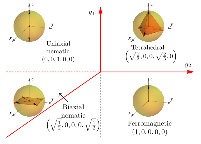
In the nematic region, where , there is an additional continuous accidental degeneracy of states with rectangular Majorana representations. A general nematic state’s order parameter can be written, up to the aforementioned symmetries, as
| (5) |
where parametrizes the degeneracy. The two states shown in Fig. 1 are representatives of higher symmetry, obtained by setting , which are referred to as uni(bi)-axial states. While all states are degenerate at the mean-field level, fluctuations lift the degeneracy through the phenomenon of order-by-disorder, selecting the uni(bi)-axial state for Song et al. (2007); Turner et al. (2007). This leads to the dotted phase boundary in Fig. 1.
Mean-field behavior in the thermodynamic limit has also been extensively investigated at non-zero in Uchino et al. (2010) leading to a number of new phases, where some of the phase boundaries with respect to and had to be numerically determined. While the ground states were invariant to changes in that remained within the same phase 222The term inert is sometimes used to describe such states Stamper-Kurn and Ueda (2013)., ground states in some of the new phases vary continuously with the parameters. Lastly and perhaps most importantly, the nematic accidental degeneracy in is lifted for any .
III Single mode approximation and exact diagonalization
III.1 Single mode Hamiltonian
In the remainder of the text we consider a tightly bound many-body system with a fixed number of particles . This implies we can write from Eq. (4) as where is the unit-normalized lowest spatial mode of the system and is the annihilation operator for a boson in this lowest spatial mode with magnetic number , since the tightness of the confining potential energetically prohibits spatially excited states. This is traditionally called the single mode approximation or SMA Law et al. (1998). For convenience we also define the vector of operators . Substituting the as above and integrating out the spatial components of the Hamiltonian Eq. (4) yields
| (6) |
plus constants. Here where and are defined in Eq. (3). The uppercase operators are obtained from their calligraphic density counterparts in Eq. (4) by letting , e.g., where still represents the -th spin matrix.
The Hamiltonians (4) and (6) evidently conserve total particle number and, as noted above, we consider it fixed at . This allows us to drop terms arising from the spatial integrals of and of Eq. (4) and to simplify the contribution of to . Hamiltonian (6) further commutes with and can thus be simultaneously diagonalized. In the remainder of this text we consider fixed eigenspaces, most often the nullspace, allowing us to drop the linear Zeeman term as in Eq. (6).
III.2 Known aspects of the quantum phase diagram
At zero quadratic Zeeman field , the exact spectrum of the tightly confined system is known Ueda and Koashi (2002). Potentially degenerate eigenlevels can be labelled by the set where is the eigenvalue of and is such that the eigenvalue of equals . can be interpreted as the number of spin-singlet pairs and as the number of bosons not in the singlet state. As mentioned above, this analogy is only a loose one, as and do not obey Bosonic commutation relations. However, the commutation relations of these and a third operator, which the authors of Ueda and Koashi (2002) denote by , can be seen to be those of the Lie algebra , closely related to that of , the spin algebra. This allows for an elegant derivation of the joint and eigenstates in analogy with the raising and lowering operator approach to the spin algebra. Technically, and are defined such that the eigenvalue of equals and . In terms of the above quantum numbers, the energies are given by
| (7) |
The easily obtained ground states show interesting parallels with the mean-field phase diagram. In the ferromagnetic region, the ground state is zero and is maximized, while in the tetrahedral region the ground state and are both zero.
The nematic-region ground state is, however, less easily reconciled with its mean-field counterparts, as the ground state is non-degenerate and unique across the entire nematic region. It consists only of singlet pairs and potentially a singlet trio, maximizing and minimizing .
On the other hand, the case where is much less well-understood analytically as or are no longer good quantum numbers. We shall focus on this regime in the following. Analytical results are obtained via the rotor mapping and contrasted with the numerical results obtained through exact diagonalization, which we briefly describe next.
III.3 Exact diagonalization
Due to the effective spatial 0-dimensionality of our tightly bound system our problem is that of diagonalizing a five-mode many-body Hamiltonian. Further fixing and , the relevant Fock bases may be enumerated by three independent occupation numbers. The sizes of the bases hence scale as with particle number making it quite feasible to diagonalize Hamiltonian (6), or at least find the ground state and its energy, at fixed values of , , and with regular desktop hardware in timescales on the order of hours for up to about 300 particles.
Denoting Fock states by
| (8) |
one way of enumerating the entire Fock basis for fixed and is by considering and as independent variables and letting and . The ranges of the independent variables are cumbersome to state but can easily be found programmatically. What remains is expressing the terms of Hamiltonian (6) with respect to this basis and diagonalizing the resulting sparse matrices, which can be accomplished with standard numerical packages.
IV The rotor mapping
Here we present the primary calculational tool allowing the derivation of analytical results of the present text, the rotor mapping. This has been introduced for spin-1 in Barnett et al. (2010) and expanded upon in Barnett et al. (2011). The latter reference also includes a brief discussion of the mapping for spin-2 systems in the absence of external fields. In this section we review the key points of the mapping in general and extend it to include an external potential for the spin-2 case. In subsection IV.1 we first comment on the natural basis of the spin-2 representation for use with the mapping and state the form of the spin matrices in it. In subsection IV.2 we briefly review the main steps of the mapping and derive the rotor Hamiltonian for our system. We comment on its properties in different regions of the parameter space, particularly Hermiticity. Subsection IV.3 outlines the process of exactly Hermitianizing the Hamiltonian in the special case when , demonstrating the equivalence of two Hermitian Hamiltonians, the many-body Hamiltonian (6) and that of a single particle on the 4-sphere in a specific potential. This subsection also introduces some of the methods employed in later sections to make approximate low-energy Hamiltonians Hermitian.
IV.1 Cartesian basis
While the canonical spin-2 matrices are complex and Hermitian, there exists a basis in which they are completely imaginary and antisymmetric. This allows one to map the original spin operators onto linear combinations of generalized angular momentum operators, significantly simplifying the analysis. The underlying reason for this is that bosonic representations of the spin group can also be thought of as representations of the real group of rotations .
There is a simple heuristic method of finding such a basis, based on transforming from standard complex spherical harmonics to real ones. We state results in terms of annihilation operators rather than the underlying single-particle basis. Using the phase convention , one arrives at the Cartesian annihilation operators:
| (9) |
Gathering these into we may neatly express parts of Hamiltonian (6) in terms of the -operators. The singlet operator becomes simply . The spin and quadratic Zeeman operators become and , where the are the pure imaginary antisymmetric spin matrices expressed in the new single-particle basis.
To state their forms concisely, let us introduce a family of simple antisymmetric matrices. Let be the 5-by-5 matrix with in the -th row and -th column, in the -th row and -th column, and elsewhere. That is, . The are then:
| (10) |
For convenience also denote .
IV.2 The rotor Hamiltonian
Next we construct the overcomplete basis 333It is evident that the basis is not orthogonal. Showing completeness is relatively straightforward but tedious.
| (11) |
where is a norm-1 5-component real vector, i.e., belonging to the 4-sphere .
It turns out that the elements of basis (11) are exactly the spatial rotations of nematic mean-field states, characterized by the order parameter in Eq. (5). More precisely, each distinct mean-field state with an order parameter of the form (where ranges over all rotations, is the matrix corresponding to in the 5-dimensional representation, and are the 5-component order parameters of Eq. (5)), can be expressed in the form of Eq. (11) with belonging to exactly one pair of diametrically opposite points on the 4-sphere.
Due to the overcompleteness of the basis, any state can be expressed as . For any particle-conserving Hamiltonian it is also possible to find an operator , interpreted as a new Hamiltonian acting on , such that is exact. The mapping consists of letting
| (12) |
as has been derived in Barnett et al. (2010). The operator acts as the gradient on functions defined on the 4-sphere and yields a vector field, lying in the tangent space to the sphere at each point. If we think of a function on as a restriction of a function on a broader subset of , the action can be expressed as .
Using the rule in Eq. (12), the norm property and the intuitive identity , we find that where is the 5-dimensional generalization of angular momentum. This in turn implies . We also find . Putting this all together and dropping constant terms yields
| (13) | |||||
Recall that . To discuss individual parts of the Hamiltonian we will also refer to the operator multiplying as .
When , the resulting Hamiltonian is Hermitian, with the ground state uniformly delocalized about the 4-sphere, which corresponds, loosely speaking, to a condensate of singlet pairs in accord with previous results Koashi and Ueda (2000); Ueda and Koashi (2002). It is interesting to comment on this result in light of the recent publication by Jen and Yip Jen and Yip (2015) who pointed out that even though naïve averaging of nematic states over rotations in all of SO produces the correct groundstates for confined antiferromagnetic spin-1 bosons, extending this to spin-2 does not work, as the singlet is no longer unique in this case. The rotor mapping demonstrates that the correct state can in fact be obtained by averaging over the associated 4-sphere.
In the general case, the obtained Hamiltonian is not Hermitian. When or when a similarity transform may be enacted which renders the transformed Hamiltonian Hermitian and which depends only on the position operators . This is the topic of the next sections. A Hermitianizing similarity transform has also been identified for the general case, but it is rather different from the one considered in this article, as it is a complicated function of the Laplacian operator. It is not at present clear whether that approach leads to similar calculational simplifications as obtained in this article and its investigation is deferred to a future publication.
For completeness, and since we shall not be using the result further, we derive in the following brief subsection the form of the Hermitianized Hamiltonian for the special case .
IV.3 Hermitianizing transform at
In this special case the Hamiltonian of Eq. (13) simplifies considerably as , arguably the most complicated term, is not present. We assume the correct similarity transform is of the form where is a function of only the position operators. We seek such that is Hermitian. The term Eq. (13) is invariant under this transformation. The Laplacian transforms as and the final non-Hermitian term of Eq. (13) picks up a Hermitian term. Gathering the evidently non-Hermitian terms and demanding that their sum be zero yields the condition
| (14) |
While one could make progress by formally solving a differential equation for on the 4-sphere derived from the above, we avoid the tedious aspects of doing so by positing that for some matrix . Inserting the ansatz into condition (14) and recalling that , we see that indeed satisfies the condition. By defining and this may be put into simple terms as . After expanding out in the remaining terms added by the transformation, the final Hamiltonian is found to be
| (15) |
V Large limits
V.1 Large positive regime
For large positive the dominant term in Hamiltonian (6) is minimized for the state , suggesting 444This state minimizes the term among all states with particles, without regard to fixing . The state obviously has , as does the limiting state (V.2) in the negative regime, suggesting the nullspace as a particularly natural choice. We consider to be fixed at 0 for the remainder of Sec. V. that the low-lying exact eigenstates are tightly localized about the poles. As shown in Barnett et al. (2011) the wave function has to have parity , so we may restrict our attention to the region about one of the poles and infer the wave function’s behaviour about the other by symmetry. We choose to expand about the pole, motivating the reparameterization
| (16) |
We take the indices of to run from to to avoid excessive arithmetic in subscripts. Next assume that low-lying states are of the form
| (17) |
where is a generic (multi)index label, is some diagonal matrix and are some residual functions of sub-exponential growth such as Hermite polynomials. The overall factor of was extracted for later convenience. The diagonal elements of can be interpreted as inverse squared oscillator lengths for the -th direction, i.e. . Our assumption of tight localization amounts to the condition , which has to be checked for consistency at the end of the calculation. Since 555Due to wave function parity such expectation values may be much less or even vanish, but the stated quantity is the upper limit on their order of magnitude., this allows us to simplify the Hamiltonian (13) by keeping only the lowest terms multiplied by each of , , and .
The goal now is to express Hamiltonian (13) in terms of and . The former follows from the coordinate definitions in Eq. (16) while the latter follows from computing where is a unit vector and is the gradient operator expressed in terms of the new coordinate system. This leads to
| (18) |
Carrying out the necessary index algebra and truncating at the lowest order terms yields the simple expressions
| (19) |
where is with the first row and column omitted. Putting this all together and letting , we obtain an approximate Hamiltonian where
| (20) |
where we do not sum over any repeated indices. The various constants in this Hamiltonian are as follows
| (21) | ||||||
where and are introduced for the purpose of later notation. This allows us to treat each direction individually. Following reasoning analogous to that of Sec. IV.3 and applying the similarity transform with we obtain a Hermitian sum of four independent harmonic oscillator Hamiltonians, i.e., a Hamiltonian of the same form as Eq. (20) but with new constants , and .
This allows us to simply read off mode energies and oscillator lengths. They are
| (22) |
where are the oscillator lengths of the Hermitianized Hamiltonian whereas are those of the original non-Hermitian Hamiltonian. The solutions are indeed of the form assumed in Eq. (17). Referring to Eq. (21) allows us to verify that and the consistency of our approach when .
The obtained mode energies agree very well with the numerically obtained spectrum. As an illustration, the largest relative discrepancy among the lowest analytically and numerically obtained energies at is percent. The accuracy of the oscillator lengths, and the wave function in general, is discussed in Sec. V.3.
It is interesting to note that the four modes agree exactly with the continuum Bogoliubov mode energies at zero momentum, minus the density mode. Stamper-Kurn and Ueda (2013) We believe this to be a nontrivial result as the number of particles does not neccessarily have to be large. Nevertheless, the limiting state about which we are expanding is of the mean-field form.
The rotor framework is also capable of describing excitations about fragmented states. This will be demonstrated in the following subsection. As stated previously, such excitations are outside the reach of conventional Bogoliubov analysis.
V.2 Large negative regime
For large negative values of , i.e., when , the dominant term in Hamiltonian (6) is minimized for the state
Note that line one of the above equation clearly demonstrates that we are working with a fragmented state, with two macroscopically occupied single-particle states for large . As mentioned before, the rotor mapping is of particular utility here.
An appropriate reparameterization in this case is
| (24) |
where we have reused the label from the case for three of the coordinates and introduced the angular variable as the fourth. Further reusing notation from the previous subsection, we assume low-energy states can be written as
| (25) |
in analogy with Eq. (17) for large positive . Here is of subexponential growth in and periodic in and . We again assume the are small, allowing us to keep only the lowest terms multiplied by each of , and . Additionally, we assume that the wave function is not localized in the direction, so that is of order 1, in the sense that its matrix elements with low-lying states are at most of order 1.
Again let and define , where we note that does not contain . The gradient components are found to be
| (26) |
Expressing components of Hamiltonian (13) in terms of and their partial derivatives and truncating higher order terms yields
| (27) |
where is with the last two columns and rows omitted. This leads to with of the same form as in Eq. (20) and the relevant constants defined as:
| (28) |
with as in Eq. (21). The rest of the calculation proceeds as in the previous section, again leading to Eq. (22) for , evaluated with the above constants, and a validation of our assumptions of localized states.
Again, the mode energies are in excellent agreement with the numerics, with the largest relative discrepancy among the first lowest energies at equal to percent.
V.3 Wave function overlaps
Besides facilitating the analytical derivation of excitation energies, the rotor mapping also yields insightful information on the wave functions themselves. The associated 4-sphere often provides a more intuitive picture of the wave function than the original second-quantized operator picture.
In this section we investigate the overlap of the ground state wave functions with arbitrary values of with wave functions in the limit of large . The ground state wave functions will be computed in two ways. In the first approach, we use the rotor mapping while with the second approach we use exact diagonalization for modest numbers of total particles. We label the wave functions with the limiting large- values as
which are appropriate for large positive and large negative , respectively. The first state has a clear correspondence to the mean-field uniaxial nematic state oriented along the -axis (c.f. Fig. 1). The second fragmented state can be viewed as an equal-weight superposition of all square biaxial nematic states lying in the plane, as is evident from Eq. (V.2). One may also view as the component of any of these mean-field ground states. For large positive or negative , one expects a large overlap of the ground state with or , respectively. On the other hand, for moderate , one may ask if any relic of the order-by-disorder phenomenon present in the continuum case, as shown in Fig. 1, remains.
The simplest expressions for the overlaps may be obtained in the regime where and is not much smaller than either or . We restrict our attention to this case in the following. This is slightly more restrictive than the condition of the previous section, namely . For the case when , but is not large compared to unity, the analysis is complicated by the interplay between asymptotic series convergence and the applicability of extending Gaussian integration limits to infinity.
We define the overlap of two possibly unnormalized states and as . States are completely determined by their wave function in the overcomplete basis and we follow the convention of labelling states of the original Hamiltonian by the same label as their rotor wave functions. That is
| (29) |
We label the ground states as obtained through the rotor mapping by . The sign in the subscript indicates whether we expanded Hamiltonian (13) about the large positive- or large negative- limiting state. We label the numerically obtained ground states by .
While the overcompleteness of the basis did not manifest itself significantly in calculating the spectrum, it does affect calculations involving the eigenfunctions. As is simple to verify from the definition of states, . In the thermodynamic limit, one can express this inner product in terms of delta functions on the four-sphere. However, for finite , overlaps must be computed by means of double integrals over the 4-sphere:
| (30) |
V.3.1 The case of positive
Here we reuse the coordinates of Sec. V.1 as defined in Eq. (16). We integrate over only half of the 4-sphere, as this is less cluttered by trivial (anti)symmetrizations. The relevant wave functions in the rotor picture (29) are and . The latter is of the form of Eq. (17) with equal to 1, i.e., , with and as expressed in Eq. (22), evaluated with the values given by Eq. (21).
In the new coordinates we have and the dot product between vectors on the four sphere is expressed as . Assuming tight localization about , the main contribution to the integral will come from that region and we may extend the boundary of integration from to . The denominator of the new integration measure varies relatively slowly, so we may set it to its value at .
Due to the simplicity of , a straightforward calculation gives
| (31) | |||||
| (32) | |||||
On the third line we approximated , permissible on account of tight localization.
Evaluation of involves the approximation (valid due to the localized wave functions) where we introduced new integration variables . With these variables and the above approximation, the integrand becomes , leading to
Combining the results of the previous paragraph and Eq. (32), we find that the total overlap can be expressed as a product of contributions from individual -directions and that the -th direction contributes a factor of . This prompts us to define
| (33) |
where the rightmost expression was derived by expanding in terms of as in Eq. (22) and letting . The are defined in Eq. (21) and are summarized here for convenience:
| (34) |
Since each direction contributes a factor of , the total overlap is
| (35) |
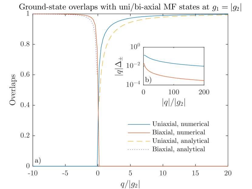
The overlap is plotted in the main panel of Fig. 2 for particles and . For comparison, we have used exact diagonalization to determine the the wave function and the overlaps for the same parameter ranges. As is expected, for large positive both the analytical and numerical overlap expressions approach unity for large . To show that the two agree in more than just this obvious large- limit, we consider their asymptotic expansions. Let and . Define . In the inset of Fig. 2 we show that tends to zero with increasing , implying that our analytical expressions agree with the numerics to at least the first order in the asymptotic expansion.
V.3.2 The case of negative
For this subsection, we reuse the and coordinates of Sec. (V.2) defined in Eq. (24). The limiting large and negative rotor wave function is . The finite- ground-state as obtained in section V.2 is , with the matrix as defined underneath Eq. (25) and the variables as defined in Eq. (22), evaluated at values from Eq. (28).
In the new coordinates, one has , with the last approximation being permissible on account of localization, as in the positive case. As before we may extend the integration boundaries to infinity. The range of integration in is from to . The dot product between vectors on the four sphere is . Since the considered wave functions do not depend on the coordinate, we may simplify integration over by a change of variables. Defining and, say, allows us to immediately perform the now trivial integral to obtain
| (36) |
where are any wave functions that do not depend on the variable, such as or . Using this expression and approximations analogous to those of Eq. (32) the simpler integrals are found to be:
| (37) | |||||
| (38) | |||||
To calculate , consider again the factor of Eq. (36). Due to the large exponent , the significant contributions to the integral will come from regions of maximum , that is for or . In both regions, we may expand to quadratic order and extend integration boundaries to infinity, yielding a Gaussian integral in where or . Also expanding the square roots and keeping lowest order terms in and yields
| (39) |
where as in the positive- case. The label equals 1 for the region and 2 for the region. The integrals over are equal in both cases, and twice the integral is in fact approximately equal to of Eq. (38), as can be verified by applying the same approximate treatment of integration over to . This leads to .
Combining the above results and expressing everything in terms of , defined in Eq. (33) and evaluated at
| (40) |
summarized after Eq. (28), ultimately yields
| (41) |
The main panel of Fig. 2 again demonstrates that both numerical and analytical overlaps tend to 1 with increasing while the inset shows that the convergence agrees to at least the first order in the asymptotic expansion.
VI Order-by-Disorder
One of the most salient features seen in Fig. 2 is the absence of the order-by-disorder phenomenon which is present for the continuum case Song et al. (2007); Turner et al. (2007). We note that while the analytical expressions for the overlaps are valid only for larger than either or , the numerically computed overlaps for modest particle number are valid for all . For the case of , one might expect a tendency towards the uniaxial nematic state for small , but this is not exhibited in Fig. 2. Instead, for small , symmetry restoring fluctuations drive the system towards the singlet state which is the true ground state for and finite particle number. Varying only affects how quickly the ground state approaches the respective limiting states. This effect is completely smooth in the whole nematic region: the smaller is, the faster the ground states approach the limiting mean-field states with increasing , without any qualitative change in behavior at .
The lack of the order-by-disorder selection at the quantum / single-mode level can be accounted for by the fact that the quadratic Zeeman potential breaks too much symmetry. Motivated by this, we consider an alternative external potential. Specifically, we consider a potential that replaces
| (42) |
in Hamiltonian (6). Such a potential could be realized with microwave fields. We note that within mean field theory, all nematic states of the form (5) are degenerate under this external potential. Considering the rotor mapping rule in Eq. (12) one can see this propagates through the mapping by changing the last line of Hamiltonian (13) to
| (43) |
In the following we will perform an analysis on this model following the rotor mapping of the previous Sections. In the Appendix, an analysis of the analogous continuum problem is discussed.
VI.1 Rotor treatment
The results of this section are similar to the large- limit in that, for sufficiently large and depending on the sign of , the rotor wave function is localized either about the pole or around the 4-5 equator of the 4-sphere. However, the localization width scales differently with than in the quadratic Zeeman case, leading to important qualitative differences. Localization at the pole (equator) also occurs at negative (positive) , which is in fact the opposite of the effect in the continuum in the absence of an external potential.
For the calculations of this section we introduce a third, more general coordinate system:
| (44) |
This can be put into a more compact form by using rotation matrices. In particular let be the matrix which rotates in the plane by angle . Then the current coordinate system can be written as . Note that . Recalling that each point of the 4-sphere is associated with a spatial rotation of a mean-field nematic state, the coordinate is seen to correspond exactly to the parameterizing the accidentally degenerate family of nematic states in Eq. (5), while and determine their spatial orientations.
As usual we consider the -nullspace, meaning that our wave functions will be independent of . By further observing factors of in Hamiltonian (13) expanded in coordinates (44) we can infer that low-lying wave functions are again localized on the scale of order in the variables. Assuming that is localized about some and denoting , we may also infer that low-lying states are localized in on a scale of order , subject to some consistency criteria. This allows us to separate the Hamiltonian into two parts, of order and of orders between to , and we discard terms of higher order in . For compact notation introduce matrices with . Denote and . Let and . Then we may write
| (45) | |||||
The last line is of a non-negligible order only when the distance between and or is of the order of or less.
Noting that does not depend on , we may tackle the above with degenerate perturbation theory. First we note that may be brought to Hermitian form by applying the similarity transformation where
| (46) |
The transformed Hamiltonian has the ground state energy
| (47) |
and ground state eigenfunction
| (48) |
where . We can then project into this low-energy subspace to obtain an effective Hamiltonian as
Now observe the following expectation value:
| (49) |
where is an arbitrary matrix. Observe that this case covers the coefficients of both the linear and quadratic terms in , Eq. (45), by choosing to be and , respectively. At this point note that should the expectation value of the linear term be of its natural order, order , completing the square in would yield another term of order 1, invalidating its placement into which is supposed to be of higher order in . Note also that the coefficient of the linear term is exactly the derivative of the zeroth-order energy from Eq. (47) with respect to . The above problem is avoided if we expand about a local extremum of , eliminating the linear term. For to be bounded from below, the extremum must be a minimum. Note that we do not get any apparent order inconsistencies if we expand about an a distance of order away from the local minimum, but the analysis is vastly simplified when the linear term is exactly zero, particularly for the last line of Eq. (45) when close to , so we focus on expansions about zeroth-order energy minima from now on.
For large enough , these occur only at and . In both of these cases, is proportional to , so both and are isotropic in . As is easy to verify, this makes the expectation values of the last line of Eq. (45) zero, eliminating those terms from . Additionally which, combined with isotropy in , leads to as well. Finally noting and and evaluating the coefficient of the quadratic term via Eq. (49), we obtain
where the upper sign corresponds to the expansion about and the lower sign about . This immediately implies the ground-state is localized about the pole, , for negative , and the 4-5 equator, , for positive . In the latter case, we may discard the term to obtain a 1-dimensional harmonic oscillator Hamiltonian. Letting , we may write the effective mode energy and oscillator length as and . In the former case, when , we may approximate , yielding a two-dimensional isotropic harmonic oscillator Hamiltonian with the angular momentum term absent. This may be solved by reintroducing the angular momentum term and then restricting to isotropic, zero-angular-momentum states. Denoting , the effective spectrum equals where and , and the oscillator length, or scale of localization in , equals .
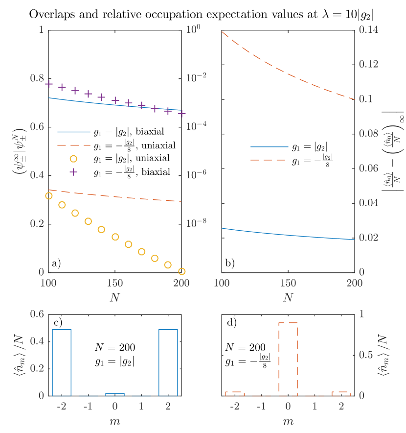
In both cases, states are seen to be localized in the direction on the scale of . It may be verified by integration over the 4-sphere, akin to the treatment in Sec. V.3, that this causes the overlaps with any mean-field state, i.e. a state of the form of Eq. (11), to tend to zero with increasing . While computationally accessible particle numbers are hardly in the large- regime, the numerical results in Fig. 3 support our analytical conclusions or, for the larger datasets, indicate the correct trend with respect to . Also shown in Fig. 3 are numerical results for the occupation numbers which verify the anaytical results of this section.
VII Conclusion
In this work, we have developed and employed the spin-2 rotor mapping formalism to obtain a number of results that have so far proven analytically inaccessible by other means. We have obtained an exact Hermitian Hamiltonian for the special case of in the presence of an arbitrary quadratic Zeeman field, and an approximate Hamiltonian in the regime for the entire nematic region. Its spectrum and localization width, the latter in the related regime, were evaluated analytically and found to be in good agreement with numerical results. Notably, for large negative the ground state tends to a fragmented condensate, the excitations about which cannot be analyzed by means of conventional Bogoliubov theory, but do lend themselves to an analysis within the rotor framework.
Additionally, one finds that no traces remain of the order-by-disorder mechanism, predicted to occur in the related continuum problem. The emergent first-order phase transition at also seems to be gone and the behaviour is smooth across the entire nematic region. Motivated by this, we considered an alternative potential which leaves the mean-field degeneracy intact, and again applied the rotor methodology. The ground state overlaps with all mean-field states are predicted to approach zero with increasing particle number, indicating we are dealing with a highly non-mean-field state. Its individual magnetic sublevel occupation values are, however, consistent with continuum order-by-disorder results.
The present analysis demonstrates that the rotor mapping may be fruitfully applied to a number of different potentials for the tightly-confined spin-2 problem. Additionally, simple analytical expressions may be obtained in the relevant limits. This makes it a suitable candidate for application to further specialized problems within the context of tightly confined spin-2 condensates. An interesting avenue for further theoretical investigation of the mapping is also the aforementioned Hermitianizing transform that may be applied in more general setups. Preliminary analysis suggests that it is indeed applicable to an arbitrary Hermitian bilinear term in the many-body Hamiltonian of Eq. (6).
Acknowledgements.
We thank Janne Ruostekoski for useful discussions during the early stages of this work. This work was supported in part by the European Union’s Seventh Framework Programme for research, technological development, and demonstration under Grant No. PCIG-GA-2013-631002.Appendix A Collective modes of continuum Hamiltonian under external field
In this Appendix, we give the collective modes of the continuum Hamiltonian described in Sec. II under the external potential given in Eq. (42). Obtaining the modes involves a straightforward but lengthy Bogoliubov analysis. Assuming we are in the nematic region of the phase diagram, we insert , where is the constant mean-field density, into the continuum Hamiltonian (with chemical potential) and expand to quadratic order in . After diagonalizing the resulting Hamiltonian, one finds the mode energies of the usual form
| (51) |
where the particular parameters for the five modes are
| (52) | ||||
| (53) |
and
| (54) | ||||
| (55) | ||||
| (56) | ||||
| (57) | ||||
| (58) |
Here, is the free particle dispersion. We next turn to an analysis of the zero-point energy due to these modes, namely where is subtracted to regularize the summation. It is found that, for sufficiently large , the biaxial nematic state is selected when while the uniaxial nematic state is selected when . This is consistent with the rotor treatment in the main text.
References
- Stamper-Kurn and Ueda (2013) D. M. Stamper-Kurn and M. Ueda, Rev. Mod. Phys. 85, 1191 (2013).
- Kawaguchi and Ueda (2012) Y. Kawaguchi and M. Ueda, Phys. Rep. 520, 253 (2012).
- Law et al. (1998) C. K. Law, H. Pu, and N. P. Bigelow, Phys. Rev. Lett. 81, 5257 (1998).
- Ho and Yip (2000) T.-L. Ho and S. K. Yip, Phys. Rev. Lett. 84, 4031 (2000).
- Koashi and Ueda (2000) M. Koashi and M. Ueda, Phys. Rev. Lett. 84, 1066 (2000).
- Mueller et al. (2006) E. J. Mueller, T.-L. Ho, M. Ueda, and G. Baym, Phys. Rev. A 74, 033612 (2006).
- Barnett et al. (2010) R. Barnett, J. D. Sau, and S. Das Sarma, Phys. Rev. A 82, 031602 (2010).
- Barnett et al. (2011) R. Barnett, H.-Y. Hui, C.-H. Lin, J. D. Sau, and S. Das Sarma, Phys. Rev. A 83, 023613 (2011).
- Lamacraft (2010) A. Lamacraft, Phys. Rev. B 81, 184526 (2010).
- Ho (1998) T.-L. Ho, Phys. Rev. Lett. 81, 742 (1998).
- Ohmi and Machida (1998) T. Ohmi and K. Machida, J. Phys. Soc. Jpn. 67, 1822 (1998).
- Chang et al. (2004) M.-S. Chang, C. D. Hamley, M. D. Barrett, J. A. Sauer, K. M. Fortier, W. Zhang, L. You, and M. S. Chapman, Phys. Rev. Lett. 92, 140403 (2004).
- Kuwamoto et al. (2004) T. Kuwamoto, K. Araki, T. Eno, and T. Hirano, Phys. Rev. A 69, 063604 (2004).
- Schmaljohann et al. (2004) H. Schmaljohann, M. Erhard, J. Kronjäger, M. Kottke, S. van Staa, L. Cacciapuoti, J. J. Arlt, K. Bongs, and K. Sengstock, Phys. Rev. Lett. 92, 040402 (2004).
- Burke et al. (1997) J. P. Burke, J. L. Bohn, B. D. Esry, and C. H. Greene, Phys. Rev. A 55, R2511 (1997).
- Ciobanu et al. (2000) C. V. Ciobanu, S.-K. Yip, and T.-L. Ho, Phys. Rev. A 61, 033607 (2000).
- Ueda and Koashi (2002) M. Ueda and M. Koashi, Phys. Rev. A 65, 063602 (2002).
- Song et al. (2007) J. L. Song, G. W. Semenoff, and F. Zhou, Phys. Rev. Lett. 98, 160408 (2007).
- Turner et al. (2007) A. M. Turner, R. Barnett, E. Demler, and A. Vishwanath, Phys. Rev. Lett. 98, 190404 (2007).
- Saito and Ueda (2005) H. Saito and M. Ueda, Phys. Rev. A 72, 053628 (2005).
- Uchino et al. (2010) S. Uchino, M. Kobayashi, and M. Ueda, Phys. Rev. A 81, 063632 (2010).
- Villain et al. (1980) J. Villain, R. Bidaux, J. P. Carton, and R. Conte, Journal de Physique 41, 1263 (1980).
- Henley (1987) C. L. Henley, J. Appl. Phys. 61, 3962 (1987).
- Henley (1989) C. L. Henley, Phys. Rev. Lett. 62, 2056 (1989).
- Wessel and Troyer (2005) S. Wessel and M. Troyer, Phys. Rev. Lett. 95, 127205 (2005).
- Wu (2008) C. Wu, Phys. Rev. Lett. 100, 200406 (2008).
- Zhao and Liu (2008) E. Zhao and W. V. Liu, Phys. Rev. Lett. 100, 160403 (2008).
- Barnett et al. (2012) R. Barnett, S. Powell, T. Graß, M. Lewenstein, and S. Das Sarma, Phys. Rev. A 85, 023615 (2012).
- You et al. (2012) Y.-Z. You, Z. Chen, X.-Q. Sun, and H. Zhai, Phys. Rev. Lett. 109, 265302 (2012).
- Zheng et al. (2013) G.-P. Zheng, L.-K. Xu, S.-F. Qin, W.-T. Jian, and J.-Q. Liang, Annals of Physics 334, 341 (2013).
- Sun and Vekua (2014) G. Sun and T. Vekua, Phys. Rev. B 90, 094414 (2014).
- Payrits and Barnett (2014) M. Payrits and R. Barnett, Phys. Rev. A 90, 013608 (2014).
- Ross et al. (2014) K. A. Ross, Y. Qiu, J. R. D. Copley, H. A. Dabkowska, and B. D. Gaulin, Phys. Rev. Lett. 112, 057201 (2014).
- Petit et al. (2014) S. Petit, J. Robert, S. Guitteny, P. Bonville, C. Decorse, J. Ollivier, H. Mutka, M. J. P. Gingras, and I. Mirebeau, Phys. Rev. B 90, 060410 (2014).
- Anglin et al. (2001) J. R. Anglin, P. Drummond, and A. Smerzi, Phys. Rev. A 64, 063605 (2001).
- Armaitis et al. (2013) J. Armaitis, R. A. Duine, and H. T. C. Stoof, Phys. Rev. Lett. 111, 215301 (2013).
- Jing et al. (2011) H. Jing, D. S. Goldbaum, L. Buchmann, and P. Meystre, Phys. Rev. Lett. 106, 223601 (2011).
- Buchmann et al. (2013) L. F. Buchmann, H. Jing, C. Raman, and P. Meystre, Phys. Rev. A 87, 031601 (2013).
- Penrose and Onsager (1956) O. Penrose and L. Onsager, Phys. Rev. 104, 576 (1956).
- Nozières, P. and Saint James, D. (1982) Nozières, P. and Saint James, D., J. Phys. France 43, 1133 (1982).
- Note (1) By a scalar potential we mean one that couples to all magnetic sublevels approximately equally, such as the potential of an optical trap and unlike that of a magnetic trap.
- Pethick and Smith (2008) C. Pethick and H. Smith, Bose-Einstein Condensation in Dilute Gases, 2nd ed. (Cambridge University Press, 2008).
- Barnett et al. (2006) R. Barnett, A. Turner, and E. Demler, Phys. Rev. Lett. 97, 180412 (2006).
- Note (2) The term inert is sometimes used to describe such states Stamper-Kurn and Ueda (2013).
- Note (3) It is evident that the basis is not orthogonal. Showing completeness is relatively straightforward but tedious.
- Jen and Yip (2015) H. H. Jen and S.-K. Yip, Phys. Rev. A 91, 063603 (2015).
- Note (4) This state minimizes the term among all states with particles, without regard to fixing . The state obviously has , as does the limiting state (V.2) in the negative regime, suggesting the nullspace as a particularly natural choice. We consider to be fixed at 0 for the remainder of Sec. V.
- Note (5) Due to wave function parity such expectation values may be much less or even vanish, but the stated quantity is the upper limit on their order of magnitude.