Effective potential method for active particles

Abstract

We investigate the steady state properties of an active fluid modeled as an assembly of soft repulsive spheres subjected to Gaussian colored noise. Such a noise captures one of the salient aspects of active particles, namely the persistence of their motion and determines a variety of novel features with respect to familiar passive fluids. We show that within the so-called multidimensional unified colored noise approximation, recently introduced in the field of active matter, the model can be treated by methods similar to those employed in the study of standard molecular fluids. The system shows a tendency of the particles to aggregate even in the presence of purely repulsive forces because the combined action of colored noise and interactions enhances the the effective friction between nearby particles. We also discuss whether an effective two-body potential approach, which would allow to employ methods similar to those of density functional theory, is appropriate. The limits of such an approximation are discussed.

I Introduction

Recently there has been an upsurge of interest towards the behaviour of the so-called active fluids whose elementary constituents are either self-propelled due their ability to convert energy into motion, for instance by chemical reactions, or receive the energy and impulse necessary to their motion when in contact with living matter, such as bacteria bechinger2016 ; marchetti2013hydrodynamics ; marchetti2015structure ; poon2013clarkia ; romanczuk2012active ; elgeti2014physics . Examples of active matter systems include self-propelled colloids, swimming bacteria, biological motors, swimming fish and flocking birds. The phenomenology of active fluids is quite different from that characterizing out-of-equilibrium molecular fluids, often referred as passive fluids, and for this reason the field is so fascinating. The theoretical studies are based on phenomenological models, constructed by using physical insight, with the aim to reproduce the complex biological mechanisms or chemical reactions determining the observed dynamics cates2012diffusive ; bialke2014negative ; fily2012athermal ; stenhammar2013continuum . Among these models we mention the important work of Cates, Tailleur and coworkers tailleur2008statistical ; cates2013active who elaborated the Run-and-Tumble (RnT) model of Berg berg2004coli and Schnitzer schnitzer1993theory . Such a model is based on the observations that the trajectories of individual bacteria consist of relatively straight segments (runs) alternated by erratic motions which cause the successive pieces of trajectory to be in almost random relative directions (tumbles). The persistence length of the trajectory sets the crossover between a ballistic regime at short time scales and a diffusive regime at longer times. Similarly chemically propelled synthetic Janus colloids have a persistent propulsion direction which is gradually reoriented by Brownian fluctuations zheng2013nongaussian (active Brownian particles). Also an ensemble of colloidal particles suspended in a ”bath” of such bacteria, is a particular realization of an active fluid maggi2014generalized ; koumakis2014delivery ; koumakis2013targeted ; maggi2011effective . Our description, at variance with the Cates and Tailleur model and the active Brownian model, involves only translational degrees of freedom of the particles, but not their orientations, and represents somehow a coarse-grained version of these models as also discussed by Farage et al. farage2015effective ; marconi2015towards . In the present model in order to capture the peculiar character of the RnT motion on a coarse-grained time scales one introduces a colored noise, that is noise with a finite memory, which represents the persistence of the motion of the bacteria.

The observed behaviour displays a relevant feature: the particles display a spontaneous tendency to aggregate even in the absence of mutual attractive forces, as a result of the combined effect of colored noise and interactions. This is a dynamic mechanism leading to a decrease of the particle effective mobility when the density increases.

Clearly this behaviour cannot be described by standard equilibrium statistical mechanics, but it is possible to make progress in our understanding by applying kinetic methods and the theory of stochastic processes marconi2010dynamic .

This paper is organized as follows: in Sec. II we present the coarse-grained stochastic model describing an assembly of active particles, consisting of a set of coupled Langevin equations for the coordinates of the particles subject to colored Gaussian noise. After switching from the Langevin description to the corresponding Fokker-Planck equation we obtain the stationary joint probability distribution of $N$ particles within the multidimensional unified colored noise approximation (MUCNA) hanggi1995colored ; cao1993effects ; maggi2015multidimensional ; marconi2015velocity . The resulting configurational distribution function can be written explicitly for a vast class of inter-particle potentials and shows the presence of non-pairwise effective interactions due to the coupling between direct forces and the colored noise. To reduce the complexity of the problem in section III we discuss whether it is possible to further simplify the theoretical study by introducing a pairwise effective potential. We analyze such an issue analytically by means of a system of just two particles in an external field and numerically using a one-dimensional system of $N$ soft repulsive spheres. Our results show the limits of the effective two-body potential method. Finally in the last section we present our conclusions. Two appendices are included: in appendix A we derive the UCNA approximation by means of multiple time-scale analysis and in B we obtain the key approximation of the theory necessary to evaluate the functional determinant of the MUCNA in the case of a many-particle system.

II Model system

In this section, we briefly describe the salient assumptions employed to formulate the model adopted in the present work. First consider an assembly of $N$ over-damped active Brownian particles at positions ${\bf r}_{i}$, self-propelling with constant velocity $v_{0}$ along orientations $\boldsymbol{n}_{i}$, which change in time according to the stochastic law

$$\dot{\boldsymbol{n}}_{i}=\sqrt{D_{r}}\boldsymbol{\eta}_{i}\times\boldsymbol{n}_{i}$$ (1)

where $\boldsymbol{\eta}_{i}(t)$ are Gaussian random processes distributed with zero mean, time-correlations $\langle\boldsymbol{\eta}_{i}(t)\boldsymbol{\eta}_{j}(t^{\prime})\rangle=2\boldsymbol{1}\delta_{ij}\delta(t-t^{\prime})$, and $D_{r}=1/\tau$ is a rotational diffusion coefficient. In addition the particles experience deterministic forces $\boldsymbol{F}_{i}=\!-\nabla_{i}{\cal U}$, generated by the potential energy ${\cal U}$. The resulting governing equations are:

$$\dot{{\bf r}}_{i}=v_{0}\,\boldsymbol{n}_{i}+\gamma^{-1}\boldsymbol{F}_{i},$$ (2)

where $\gamma$ is the friction coefficient. The resulting dynamics are persistent on short time scales, i.e. the trajectories maintain their orientation for an average time $\tau$, and diffusive on larger time scales. Hydrodynamic interactions are disregarded for the sake of simplicity together with inertial effects because particles are typically in a low-Reynolds-number regime purcell1977life .

Equations (1) and (2) involve the dynamics of both translational and rotational degrees of freedom and are not a practical starting point for developing a microscopic theory. Hence, it is convenient to switch to a coarse-grained description stochastically equivalent to the original one on times larger than $\tau$ . To this purpose, one integrates out the angular coordinates as shown by Farage et al.farage2015effective . According to this approximation, one introduces a colored stochastic noise term acting on the position coordinates and replacing the stochastic rotational dynamics (1). The effective evolution equations are:

$$\dot{{\bf r}}_{i}(t) =\frac{1}{\gamma}\boldsymbol{F}_{i}(t)+\boldsymbol{u}_{i}(t),$$ (3)

with

$$\dot{\boldsymbol{u}}_{i}(t)=-\frac{1}{\tau}\boldsymbol{u}_{i}(t)+\frac{D^{1/2}}{\tau}\boldsymbol{\eta}_{i}(t)$$ (4)

where $\boldsymbol{u}_{i}(t)$ is an Ornstein-Uhlenbeck process with zero mean, time-correlation function given by:

$$\langle\boldsymbol{u}_{i}(t)\,\boldsymbol{u}_{j}(t^{\prime})\rangle=\frac{D}{\tau}e^{-2|t-t^{\prime}|/\tau}\boldsymbol{1}\delta_{ij}.$$ (5)

and whose diffusion coefficient $D$ is related to the original parameters by $D=v_{0}^{2}\tau/6$. In order to derive an equation involving only the positions of the particles we differentiate with respect to time eq.(3) and with simple manipulations we get the following second order differential equation:

$$\ddot{x}_{i}=\frac{1}{\gamma}\sum_{k}\frac{\partial F_{i}}{\partial x_{k}}\dot{x}_{k}-\frac{1}{\tau}\left[\dot{x}_{i}-\frac{F_{i}}{\gamma}\right]+\frac{D^{1/2}}{\tau}\eta_{i}(t)$$ (6)

where for the sake of notational economy we indicated by $x_{i}$ the array $\{{\bf r}_{i}\}$ and similarly the components of the force. By performing an adiabatic approximation (see appendix A) we neglect the terms $\ddot{x}_{i}$ and obtain the following set of Langevin equations for the particles coordinates:

$$\dot{x}_{i}\simeq\sum_{k}\Gamma^{-1}_{ik}\Bigl{[}\frac{1}{\gamma}F_{k}+D^{1/2}\eta_{k}(t)\Bigl{]}$$ (7)

with the non dimensional friction matrix $\Gamma_{ik}$ defined as

$$\Gamma_{ik}(x_{1},\dots,x_{N})=\delta_{ik}+\frac{\tau}{\gamma}\frac{\partial^{2}{\cal U}(x_{1},\dots,x_{N})}{\partial x_{i}\partial x_{k}}.$$ (8)

Notice that, within the approximation introduced in eq. (7), the effective random force corresponds to a multiplicative noise due to its dependence on the state of the system, $x_{i}(t)$, through the prefactor $\Gamma^{-1}_{ik}(x_{1},\dots,x_{N})$ in front of the noise term $\eta_{k}(t)$.

For the sake of concreteness ${\cal U}$ is the sum of one-body and two body contributions:

$${\cal U}(x_{1},\dots,x_{N})=\sum_{i}u(x_{i})+\sum_{i>j}w(x_{i},x_{j}).$$ (9)

The associated multidimensional Smoluchowski equation for the the configurational distribution function associated with eq. (7) can be written as (see ref. marconi2015towards ):

$$\frac{\partial P_{N}(x_{1},\dots,x_{N};t)}{\partial t}=-\sum_{l}\frac{\partial}{\partial x_{l}}\sum_{k}\Gamma^{-1}_{lk}\Bigl{(}\frac{1}{\gamma}F_{k}P_{N}-D\sum_{j}\frac{\partial}{\partial x_{j}}[\Gamma^{-1}_{jk}P_{N}]\Bigr{)}$$ (10)

and shows that the effective friction experienced by each particle also depends on the coordinates of all other particles. In order to determine the stationary properties of the model we apply the following zero current condition in eq. (10) and get:

$$-T_{s}\sum_{\beta}\sum_{n}\frac{\partial}{\partial r_{\beta n}}[\Gamma^{-1}_{\alpha l,\beta n}({\bf r}_{1},\dots,{\bf r}_{N})P_{N}({\bf r}_{1},\dots,{\bf r}_{N})]$$

$$=P_{N}({\bf r}_{1},\dots,{\bf r}_{N})\Bigl{(}\frac{\partial u({\bf r}_{\alpha l})}{\partial r_{\alpha l}}+\sum_{k\neq l}\frac{\partial w({\bf r}_{l}-{\bf r}_{k})}{\partial r_{\alpha l}}\Bigl{)}\,.$$ (11)

The resulting stationary distribution can be written explicitly as (see ref. maggi2015multidimensional ):

$$P_{N}(x_{1},\dots,x_{N})=\frac{1}{Z_{N}}\,\exp\Bigl{(}-\frac{{\cal H}(x_{1},\dots,x_{N})}{T_{s}}\Bigr{)}$$ (12)

where we have defined the effective temperature $T_{s}=D\gamma$ and the effective configurational energy of the system ${\cal H}(x_{1},\dots,x_{N})$ related to the bare potential energy ${\cal U}(x_{1},\dots,x_{N})$ by:

$${\cal H}(x_{1},\dots,x_{N})={\cal U}(x_{1},\dots,x_{N})+\frac{\tau}{2\gamma}\sum_{k}^{N}\Bigr{(}\frac{\partial{\cal U}(x_{1},\dots,x_{N})}{\partial x_{k}}\Bigl{)}^{2}-T_{s}\ln|\det\Gamma_{ik}|,$$ (13)

where $Z_{N}$ is a normalization constant

$$Z_{N}=\mathrm{Tr}\exp\left[-\frac{{\cal H}({\bf r}_{1},\dots,{\bf r}_{N})}{T_{s}}\right].$$ (14)

with $\mathrm{Tr}\equiv\int d{\bf r}_{1},\dots,d{\bf r}_{N}$. Formula (12), gives within the unified colored noise approximation, a complete information about the configurational state of a system of $N$ particles, but it requires the evaluation of a $dN\times dN$ determinant stemming from the matrix $\Gamma_{ik}$, where $d$ is the dimensionality of the system. One can only get analytic results either by considering non-interacting systems with $d=1,..,3$ or systems with few particles, where the computation of the determinant is possible. Thus, in spite of the fact that in principle from the knowledge of $P_{N}$ is possible to determine all steady properties of the system, including the pair correlation function of the model, $g({\bf r}_{1},{\bf r}_{2})$, this task is not possible in practice. The same situation occurs in equilibrium statistical mechanics where from the knowledge of the canonical Boltzmann distribution of an $N$ particle system we cannot in general exactly determine the n-particle distribution functions with $n<N$. On the other hand, it is possible to derive a structure similar to the Born-Bogolubov-Green-Yvon (BBGY) hierarchy of equations linking the n-th order distribution to those of higher order, but it requires the specification of a closure relation. To this purpose, we integrate eq. (11) over $d(N-n)$ coordinates and obtain an equation for the marginalized probability distributions of $n$ particles, $P_{N}^{(n)}({\bf r}_{1},\dots,{\bf r}_{n})$ in terms of higher order marginal distributions. When $n=1$ we find:

$$T_{s}\int\int d{\bf r}_{2}\dots d{\bf r}_{N}\sum_{\beta=1}^{d}\sum_{n=1}^{N}\frac{\partial}{\partial r_{\beta n}}[\Gamma^{-1}_{\alpha 1,\beta n}({\bf r}_{1},\dots,{\bf r}_{N})P_{N}({\bf r}_{1},\dots,{\bf r}_{N})]=$$

$$-P^{(1)}_{N}({\bf r}_{1})\frac{\partial u({\bf r}_{1})}{\partial r_{\alpha 1}}-(N-1)\int d{\bf r}_{2}P^{(2)}_{N}({\bf r}_{1},{\bf r}_{2})\frac{\partial w({\bf r}_{1}-{\bf r}_{2})}{\partial r_{\alpha 1}}$$ (15)

where Greek indexes stand for Cartesian components.

In the case of a large number of particles the exact matrix inversion necessary to use formula (15) becomes prohibitive. However, we notice that in the limit of small $(\tau/\gamma)$ and $N\to\infty$ the structure of the matrix $\Gamma^{-1}_{\alpha 1,\beta n}$ becomes much simpler as illustrated in appendix B and can be approximated by

$$\Gamma^{-1}_{\alpha l,\beta n}({\bf r}_{l})\approx\Bigl{(}\delta_{\alpha\beta}-\frac{\tau}{\gamma}u_{\alpha\beta}({\bf r}_{l})-\frac{\tau}{\gamma}\sum_{k\neq l}w_{\alpha\beta}({\bf r}_{l}-{\bf r}_{k}))\Bigl{)}\delta_{ln},$$

where $u_{\alpha\beta}\equiv\frac{\partial^{2}u({\bf r})}{\partial r_{\alpha}\partial r_{\beta}}$ and $w_{\alpha\beta}\equiv\frac{\partial^{2}w({\bf r})}{\partial r_{\alpha}\partial r_{\beta}}$. Substituting this approximation in eq. (15) we get:

$$T_{s}\sum_{\beta}\frac{\partial}{\partial r_{\beta 1}}\Bigl{[}P^{(1)}_{N}({\bf r}_{1})\delta_{\alpha\beta}-\frac{\tau}{\gamma}P^{(1)}_{N}({\bf r}_{1})u_{\alpha\beta}({\bf r}_{1})-(N-1)\frac{\tau}{\gamma}\int\sum_{k}d{\bf r}_{2}P^{(2)}_{N}({\bf r}_{1},{\bf r}_{2})w_{\alpha\beta}({\bf r}_{1}-{\bf r}_{2})\Bigl{]}$$

$$=-P^{(1)}_{N}({\bf r}_{1})\frac{\partial u({\bf r}_{1})}{\partial r_{\alpha 1}}-(N-1)\int d{\bf r}_{2}P^{(2)}_{N}({\bf r}_{1},{\bf r}_{2})\frac{\partial w({\bf r}_{1}-{\bf r}_{2})}{\partial r_{\alpha 1}}$$ (16)

Such an equation, once a prescription for $P^{(2)}_{N}({\bf r}_{1},{\bf r}_{2})$ is specified, can be used to derive the density profile of a system of interacting particles under inhomogeneous conditions. Let us remark that eq. (16) expresses the condition of mechanical equilibrium equivalent to the first member of the BBGY hierarchy as discussed in ref. marconi2015towards .

III Effective potential

Let us apply eq.(11) to a system a system comprising just two particles so that the equation becomes closed:

$$T_{s}\sum_{\beta=1}^{d}\sum_{n=1}^{2}\frac{\partial}{\partial r_{\beta n}}[\Gamma^{-1}_{\alpha 1,\beta n}({\bf r}_{1},{\bf r}_{2})P^{(2)}_{2}({\bf r}_{1},{\bf r}_{2})]=-P^{(2)}_{2}({\bf r}_{1},{\bf r}_{2})\Bigl{(}\frac{\partial u({\bf r}_{1})}{\partial r_{\alpha 1}}+\frac{\partial w({\bf r}_{1}-{\bf r}_{2})}{\partial r_{\alpha 1}}\Bigr{)}\,.$$

(17)

The solution is

$$P^{(2)}_{2}({\bf r}_{1},{\bf r}_{2})=\frac{1}{Z_{2}}\exp\Bigl{(}-\frac{\psi({\bf r}_{1},{\bf r}_{2})+\frac{\tau}{2\gamma}\sum_{\alpha=1}^{d}[\frac{\partial}{\partial r_{\alpha}}\psi({\bf r}_{1},{\bf r}_{2}))]^{2}-D\gamma\ln\det\Gamma({\bf r}_{1},{\bf r}_{2})}{T_{s}}\Bigr{)}$$ (18)

where $\psi({\bf r}_{1},{\bf r}_{2})=u({\bf r}_{1})+u({\bf r}_{2})+w({\bf r}_{1}-{\bf r}_{2})$ and $\det\Gamma$ is the determinant associated with the $2d\times 2d$ matrix whose elements are

$$\Gamma_{\alpha\beta}({\bf r}_{i},{\bf r}_{j})=\delta_{\alpha\beta}\delta_{ij}+\frac{\tau}{\gamma}\frac{\partial^{2}\psi({\bf r}_{i},{\bf r}_{j})}{\partial r_{\alpha i}\partial r_{\beta j}}$$ (19)

with $i,j=1,2$. The form of eq. (18) suggests the idea of introducing an effective potential to describe the interaction experienced by the particles when subjected to colored noise. The effective potential can simplify the description, make the analysis more transparent and avoid the difficulty of evaluating the inverse matrix $\Gamma$ when the system comprises a large number of particles. However, we must explore the validity of such a method since it involves an approximate treatment of the interactions when $N\geq 3$. Let us begin with the simplest case of just two particles free to move on a line in the absence of external fields and write the pair distribution. To this purpose let us consider the $2\times 2$ matrix $\Gamma_{ij}$:

$$\Gamma^{(2)}=\left(\begin{array}[]{ccccccc}1+\frac{\tau}{\gamma}w_{11}(x_{1}-x_{2})&-\frac{\tau}{\gamma}w_{11}(x_{1}-x_{2})\\ -\frac{\tau}{\gamma}w_{11}(x_{1}-x_{2})&1+\frac{\tau}{\gamma}w_{11}(x_{1}-x_{2})\end{array}\right)$$

with $w_{11}=\frac{d^{2}w(x_{1}-x_{2})}{dx_{1}^{2}}$ . The resulting two particles distribution function $P_{2}^{(2)}$ has the form:

$$P_{2}^{(2)}(x_{1}-x_{2})=\frac{1}{Z_{2}}\exp\Bigl{(}-\frac{\phi(x_{2}-x_{1})}{T_{s}}\Bigl{)}$$ (20)

Thus, we can define, apart from a constant, the following pair effective potential by taking the logarithm of $P_{2}$

$$\phi(x_{1}-x_{2})=w(x_{1}-x_{2})+(\frac{\tau}{\gamma})[w_{1}(x_{1}-x_{2})]^{2}-D\gamma\ln(1+2(\frac{\tau}{\gamma})w_{11}(x_{1}-x_{2}))$$ (21)

with $w_{1}=\frac{dw(x_{1}-x_{2})}{dx_{1}}$.

The above result can be generalized in the case of higher dimensionality. The pair correlation function in $d$ dimensions for a two-particle system interacting via a central potential $w(r)$, in the absence of external potentials, reads:

$$g(r)=\exp\left(-\frac{w(r)+\frac{\tau}{\gamma}[w^{\prime}(r)]^{2}-T_{s}\ln[(1+2\frac{\tau}{\gamma}w^{\prime\prime}(r))(1+2\frac{\tau}{\gamma}\frac{w^{\prime}(r)}{r})^{d-1}]}{T_{s}}\right)$$ (22)

where the primes mean derivative with respect to the separation $r$. Thus the effective pair potential reads $\phi(r)=-T_{s}\ln g(r)$. Let us remark that the effective potential, being derived in the low-density limit, does not account for the three body terms which instead are present if one considers formula (12) with $N>2$.

In all these cases the dependence of $\phi$ on the effective temperature is quite interesting because as $D$ increases the effective potential displays a deeper and deeper potential well. Hereafter, we shall adopt the following unit system: lengths are expressed in terms of the molecular length $\sigma$, time in terms of the unit time $\gamma^{-1}$ and the unit mass is set equal to 1.

In particular, we find that for a pair potential $w(x)=w_{0}(\frac{\sigma}{x})^{12}$, in order to observe an attractive region it is necessary to have $2D\tau/\sigma^{2}>1$. This is shown in Fig. 1 where we display the pair correlation function obtained by numerical simulations of a system of repulsive particles in one dimension for different values of $D$, average density $\rho\sigma=0.25$ and for $\tau=0.1$. The various curves correspond to different values of $D$ and one can see that the height of the peak increases with $D$ because the effective attraction increases. Such an effective attraction in a system where only repulsive interparticle forces are in action is due to a dynamical mechanism. It can be understood as follows: the friction that a particle experiences with the background fluid is enhanced by the presence of surrounding particles so that their mobility decreases. Being less mobile the particle tends to spend more time in configurations where it is closer to other particles and one interprets this situation as an effective attraction cates2013active ; cates2014motility ; barre2014motility .

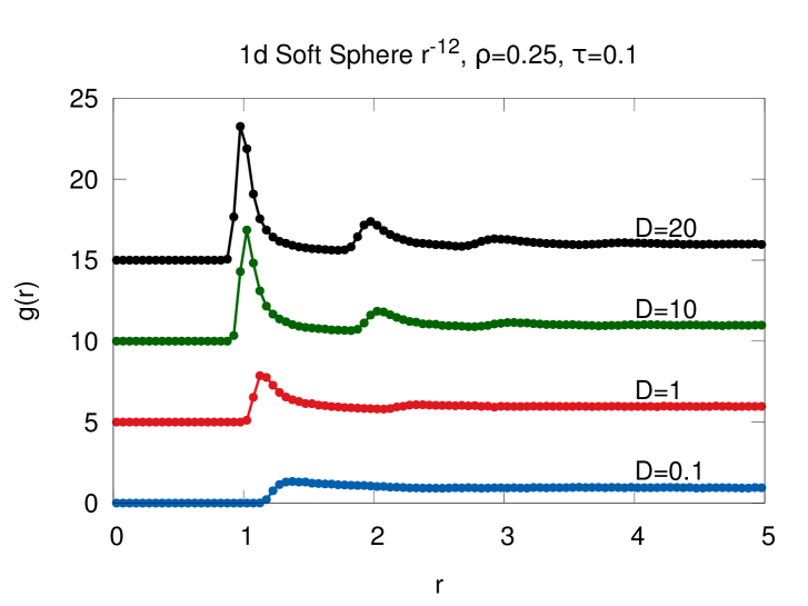
Figure 1: Results for the pair correlation function obtained via numerical simulation of a 1 dimensional system. Density $\rho$ is expressed in units $\sigma^{-1}$, $\tau$ in units $\gamma^{-1}$ and $D$ in units $T_{s}/\gamma$.

In spite of the fact that the MUCNA N-particle distribution function is known it is difficult to apply it to large systems because of the many-body nature of the interactions. On the other hand, if one could replace the complicated MUCNA potential by an effective pairwise potential it would possible to use all the machinery employed in the study of molecular fluids. Under this hypothesis one could, for instance, use methods such as the density functional method, define a Helmholtz intrinsic free energy, or utilize the integral equations method and greatly simplify the study the phase behavior of the model. To analyze its validity, we use a simple example: consider an interacting two-particle system subjected to the action of an external potential $u(x)$ whose distribution function is given by

$$P_{2}^{(2)}(x_{1},x_{2})=\frac{1}{Z_{2}}\,\exp\Bigl{(}-\frac{w(x_{1},x_{2})+(u(x_{1})+u(x_{2})}{T_{s}}\Bigr{)}$$

$$\times\exp\Bigl{(}-\frac{\tau}{2\gamma T_{s}}[\frac{\partial}{\partial x_{1}}(w(x_{1},x_{2})+u(x_{1}))]^{2}-\frac{\tau}{2\gamma T_{s}}[\frac{\partial}{\partial x_{2}}(w(x_{1},x_{2})+u(x_{2}))]^{2}$$

$$+\ln\det\Gamma(x_{1},x_{2})\Bigr{)}$$ (23)

with

$$\det\Gamma(x_{1},x_{2}) = 1+\frac{\tau}{\gamma}\Bigl{(}2\frac{\partial^{2}w(x_{1},x_{2})}{\partial x_{1}^{2}}+\frac{\partial^{2}u(x_{1})}{\partial x_{1}^{2}}+\frac{\partial^{2}u(x_{2})}{\partial x_{2}^{2}}\Bigr{)}$$

$$+(\frac{\tau}{\gamma})^{2}\Big{(}\frac{\partial^{2}w(x_{1},x_{2})}{\partial x_{1}^{2}}[\frac{\partial^{2}u(x_{1})}{\partial x_{1}^{2}}+\frac{\partial^{2}u(x_{2})}{\partial x_{2}^{2}}]+\frac{\partial^{2}u(x_{1})}{\partial x_{1}^{2}}\frac{\partial^{2}u(x_{2})}{\partial x_{2}^{2}}\Bigr{)}.$$

In the spirit of the effective potential idea we introduce the following superposition approximation

$$P_{2}^{approx}(x_{1},x_{2})\approx\frac{1}{\ Z_{2}^{approx}}\,\exp\Bigl{(}-\frac{w(x_{1},x_{2})+u(x_{1})+u(x_{2})}{T_{s}}\Bigr{)}$$

$$\times\exp\Bigl{(}-\frac{\tau}{2\gamma T_{s}}[\frac{\partial}{\partial x_{1}}w(x_{1},x_{2})]^{2}-\frac{\tau}{2\gamma T_{s}}[\frac{\partial}{\partial x_{2}}w(x_{1},x_{2})]^{2}-\frac{\tau}{2\gamma T_{s}}[\frac{\partial}{\partial x_{1}}u(x_{1})]^{2}-\frac{\tau}{2\gamma T_{s}}[\frac{\partial}{\partial x_{2}}u(x_{2})]^{2}$$

$$+\ln\det\Gamma^{approx}(x_{1},x_{2})\Bigr{)}$$ (25)

with

$$\ln\det\Gamma^{approx}(x_{1},x_{2})\approx\ln\Bigl{(}1+2(\frac{\tau}{\gamma})\frac{\partial^{2}w(x_{1},x_{2})}{\partial x_{1}^{2}}\Bigr{)}+\ln\Bigl{(}1+(\frac{\tau}{\gamma})\frac{\partial^{2}u(x_{1})}{\partial x_{1}^{2}}\Bigr{)}+\ln\Bigl{(}1+(\frac{\tau}{\gamma})\frac{\partial^{2}u(x_{2})}{\partial x_{2}^{2}}\Bigr{)}.$$ (26)

Clearly the exact formula and the approximation for the determinant differ beyond the linear order in $\tau/\gamma$, but perhaps the largest discrepancy occurs in the presence of cross terms of linear order in $\tau/\gamma$, such as $w(x_{1},x_{2})u(x_{1})$ in the interaction potential . A test can be performed by comparing the probability density profile $P^{(1)}(x_{1})$ obtained by integrating over the coordinate $x_{2}$ the exact distribution and the one obtained by applying the same procedure to the approximate distribution (25). The comparison, displayed in Fig. 2, reveals the presence of a systematic shift of the second peak of the approximate distribution towards larger distances from the confining wall, as if the total effective force were more repulsive.

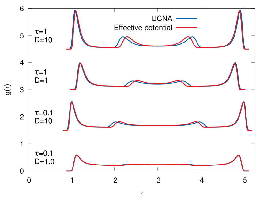
Figure 2: Normalized single particle probability distribution function for a one dimensional system two interacting particles confined between two repulsive walls at $x=0$ and $x=6$. The wall repulsive potential is $u(x)=u_{0}(\frac{\sigma}{x})^{12}$ at each wall and $w(x_{1}-x_{2})=w_{0}(\frac{\sigma}{(x_{1}-x_{2})})^{12}$ between the particles with $u_{0}=w_{0}=1$. The curves refer to $\tau=0.1,1.$ and $D=1,10$ expressed in the same units as in fig. 1. The agreement between the Gaussian colored noise result and the effective potential is poor as far as the second peak is concerned: its position is shifted towards larger distances from the wall, when the persistence time increases.

We turn, now, to consider a many-particle systems and perform a similar comparison. We have simulated the system described by eqs. (3) - (4) with $N=1000$ and computed numerically the pair correlation function. In order to check the effective potential approximation we also performed simulations of the over-damped Langevin equation with white noise for particles in one dimension subjected to interactions given by $\phi(x_{i}-x_{j})$ . The corresponding results are shown in figs. 3-6. One observes in figs. 3 and 4 that at moderately low values of the persistence time, $\tau=0.1$, the discrepancy between the effective potential approximation and the full colored noise result is not too large even at large densities, although there is a systematic shift of the peaks in the effective potential towards larger values of the distance. The situation at values of $\tau$ ten times larger, $\tau=1$, and $D=0.1$ and $10$ is remarkably worse and the peaks of the effective theory display a much larger shift as illustrated by figs. 5-6. Such a shift is determined by the approximate treatment of the three-body repulsive term which appears in eq. (13) which becomes more relevant as the density and $\tau$ increase. These findings pose some limits to the possibility of obtaining reliable results by employing the effective potential approximation for values of the persistence time too large.

III.1 Van der Waals free energy

We use, now, a van der Waals (vdW) argument to estimate the free energy for the present model in $d$-dimension when the bare potential is of the form $w(r)=w_{0}(\frac{\sigma}{r})^{\alpha}$ and identify the following repulsive contribution in the effective potential:

$$\phi_{rep}(\tilde{r})=w_{0}(\frac{\sigma}{r})^{\alpha}+\frac{\tau}{\gamma}\frac{\alpha^{2}}{\sigma^{2}}w_{0}^{2}(\frac{\sigma}{r})^{2\alpha+2}$$ (27)

whereas the attractive contribution is:

$$\phi_{attr}(r)=-T_{s}\ln\Bigl{(}\Bigl{[}1+2\alpha(\alpha+1)\frac{w_{0}\tau}{\gamma\sigma^{2}}(\frac{\sigma}{r})^{\alpha+2}\Bigr{]}\Bigl{[}1-2\alpha\frac{w_{0}\tau}{\gamma\sigma^{2}}(\frac{\sigma}{r})^{\alpha+2}\Bigr{]}^{d-1}\Bigl{)}.$$ (28)

Thus for $w_{0}\frac{\tau}{\gamma\sigma^{2}}<<1$ the system reduces to a system of passive soft repulsive spheres. Using a standard procedure we represent the free energy as the sum of a repulsive contribution evaluated in the local density approximation plus a non local mean-field attractive term:

$${\cal F}[\rho^{(1)}]=T_{s}\int d^{d}r\rho({\bf r})\Bigl{[}\ln\Bigl{(}\frac{\rho^{(1)}({\bf r})}{1-b\rho^{(1)}({\bf r})}\Bigr{)}-1\Bigr{]}+\frac{1}{2}\iint_{|{\bf r}-{\bf r}^{\prime}|>R_{b}}d^{d}rd^{d}r^{\prime}\,\phi_{attr}({\bf r}-{\bf r}^{\prime})\rho^{(1)}({\bf r})\rho({\bf r}^{\prime})$$

(29)

where $b=\omega_{d}R^{d}$, $\omega_{d}=1,\pi/2,2\pi/3$ for $d=1,2,3$, respectively and the effective hard-sphere diameter, $R_{b}$ is given by the Barker-Henderson formula:

$$R_{b}=\int_{0}^{\infty}dr(1-e^{-\phi_{rep}(\tilde{r})/T_{s}}).$$ (30)

Following the standard vdW approach we may represent the pressure associated with the functional (29) as:

$$p=\frac{T_{s}\,\rho}{1-b\rho}-a\rho^{2},$$ (31)

where the value of the coefficient $a$ is determined by the strength of the effective attractive interaction:

$$a=-\int_{R_{b}}^{\infty}d^{d}r\,\phi_{attr}(r).$$ (32)

From the form of the effective attractive potential (28) one sees that $a$ is an increasing function of the non dimensional parameter $\frac{w_{0}\tau}{\gamma\sigma^{2}}$ and of $T_{s}$. The latter feature determines a remarkable difference with respect to passive fluids: in that case the vdW pressure is the sum of an entropic term proportional to the temperature and of a negative temperature independent enthalpic term. In active fluids, on the contrary, the coefficient $a$ increases roughly linearly with $T_{s}$ as the entropic term does. As a result, $T_{s}$, since $a/T_{s}$ is nearly constant, does not play a major role in determining the critical parameters of the active model. The effective attraction among the particles has its origin in the reduction of their mobility, reflected by the presence of an effective friction $\Gamma_{ij}$ in (7) which increases with increasing density. As a result the particles tend to accumulate where their density is higher and move more slowly and possibly lead to the mobility induced phase separation phenomenon.

In analogy with the vdW model of passive fluids one can determine the critical parameters, where a second order transition would take place, by solving simultaneously the equations $\frac{\partial p}{\partial V}=0$ and $\frac{\partial^{2}P}{\partial V^{2}}=0$ with the result:

$$\frac{a(\tau_{c})}{T_{s}}=\frac{27}{8}b\,,\,\,\,\,\,\,\rho_{c}=\frac{1}{3b}$$ (33)

Thus, in order to have phase separation, the persistence time, $\tau$, must exceed the critical value $\tau_{c}$, implicitly given by the first of equations (33). However, the numerical investigation of the phase separation of Gaussian-colored noise driven particles is still in progress and so far it has not revealed a clear phase separation in the absence of attraction.

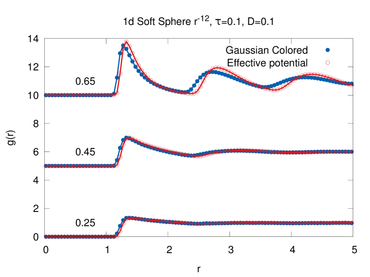
Figure 3: Numerical simulation of a 1 dimensional system. Pair correlation for $\rho\sigma=0.25,0.45,0.65$ for fixed $\tau=0.1$ and $D=0.1$ , expressed in the same units as in fig. 1. The height of the peak increases with density. The agreement between the Gaussian colored noise result and the effective potential is moderately good.

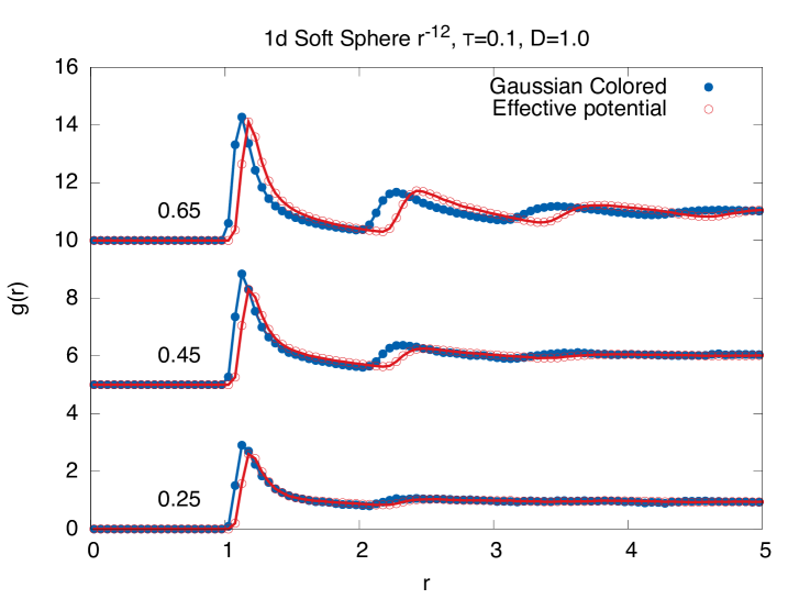
Figure 4: Numerical simulation of a 1 dimensional system. Pair correlation for $\rho\sigma=0.25,0.45,0.65$ for fixed $\tau=0.1$ and $D=1$, expressed in the same units as in fig. 1. The agreement between the Gaussian colored noise result and the effective potential is rather poor due to the relatively large value of the persistence time.

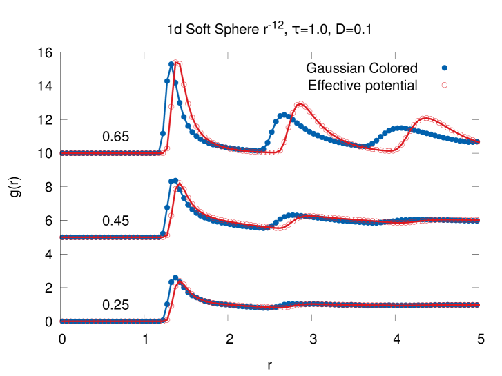
Figure 5: Numerical simulation of a 1 dimensional system. Pair correlation for $\rho\sigma=0.25,0.45,0.65$ for fixed $\tau=1.$ and $D=0.1$ The agreement between the Gaussian colored noise result and the effective potential is rather poor due to the relatively large value of the persistence time.

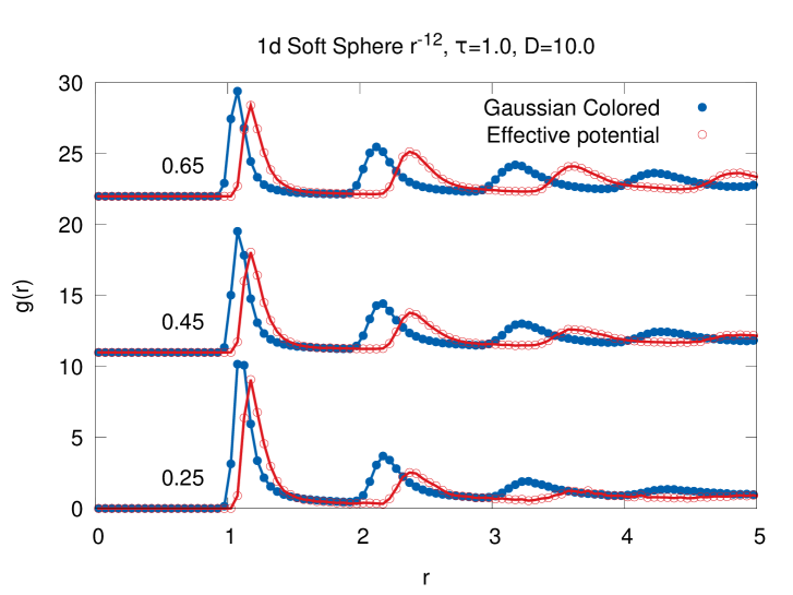
Figure 6: Numerical simulation of a 1 dimensional system. Pair correlation for $\rho\sigma=0.25,0.45,0.65$ for fixed $\tau=1.$ and $D=10.$ The agreement between the Gaussian colored noise result and the effective potential is rather poor due to the relatively large value of the persistence time.

IV Conclusions

We discussed the properties of a newly introduced model describing an active fluid, consisting of an an assembly of repulsive soft spheres subject to over-damped dynamics and driven by a colored noise. Although within the MUCNA is possible to get an analytical expression for the many-particle distribution function it is difficult to make progress without resorting to approximations. The effective potential hypothesis represents a practical possibility since it reduces the many-body potential to a pairwise additive potential where one can use the standard tools of statistical mechanics. To test the hypothesis, we performed two checks. In the first we employed a toy model consisting of just two particles in an external field and performed explicitly the analytic calculations. In the second check, we compared by numerical Brownian simulation the properties of a one-dimensional system of soft repulsive spheres subjected to colored noise against the corresponding properties of a system of particles interacting via the effective potential. It is found that for values of the persistence time, not too large the effective potential approximation is reliable.

V Acknowledgements

C. M. acknowledges support from the European Research Council under the European Union?s Seventh Framework programme (FP7/2007-2013)/ERC Grant agreement No. 307940. M.P. acknowledges support from NSF-DMR-1305184.

Appendix A Derivation of the UCNA equation by multiple time-scale analysis

In this appendix we derive the UCNA approximation by a multiple time-scale analysis following the same method employed in ref. marconi2006nonequilibrium ; marini2007 . It allows to derive in a systematic fashion the configurational Smoluchowski equation from the Kramers equation via the elimination of the velocity degrees of freedom. To achieve this goal one introduces fast and slow time-scale variables for the independent variable, and subsequently treats these variables, fast and slow, as if they are independent. The solution is first expressed as a function of these different time scales and subsequently these new independent variables are used to remove secular terms in the resulting perturbation theory. Physically speaking, the fast scale corresponds to the time interval necessary to the velocities of the particles to relax to configurations consistent with the values imposed by the vanishing of the currents. The slow time scale is much longer and corresponds to the time necessary to the positions of the particles to relax towards the stationary configuration.

It is convenient to work with non dimensional quantities and introduce the following variables:

$$\bar{t}\equiv t\frac{v_{T}}{l},\qquad V\equiv\frac{v}{v_{T}},\qquad X\equiv\frac{x}{l},\qquad\Gamma=\gamma\frac{l}{v_{T}},\qquad\zeta=\frac{l}{\tau v_{T}}$$ (34)

$$K(X)\equiv\frac{lF(x)}{mv_{T}^{2}},\qquad v_{T}=\sqrt{D/\tau}$$ (35)

where $l$ is a typical length of the problem, such as the size of the particles and $\zeta$ plays the role of a non dimensional friction.

It is clear that if $\zeta>>1$ particles lose memory of their initial velocities after a time span which is of the order of the time constant $\tau$ so that the velocity distribution soon becomes stationary. We shall assume that $\gamma\tau$ stays finite when $\tau\to 0$. In this limit the Smoluchowski description of a system of non interacting particles, which takes into account only the configurational degrees of freedom, turns out to be adequate. However, for intermediate values of $\tau$ the velocity may play a role. The question is how do we recover the UCNA starting from a description in the larger space $x,v$ ? We rewrite Kramers’ evolution equation for the phase-space distribution function using (34-35) as:

$$\frac{\partial\tilde{f}(X,V,\bar{t})}{\partial\bar{t}}+V\frac{\partial}{\partial X}\tilde{f}(X,V,\bar{t})+\frac{\zeta}{\Gamma}K(X,\bar{t})\frac{\partial}{\partial V}\tilde{f}(X,V,\bar{t})=\zeta L_{FP}\tilde{f}(X,V,\bar{t})$$ (36)

having introduced the “Fokker-Planck” operator

$$L_{FP}\tilde{f}(X,V,\bar{t})=\frac{\partial}{\partial V}\Bigl{[}\frac{\partial}{\partial V}+s(X)V\Bigl{]}\tilde{f}(X,V,\bar{t})$$ (37)

with

$$s(X)=1-\frac{1}{\Gamma\zeta}\frac{dK}{dX}$$

whose eigenfunctions are

$$H_{\nu}(X,V)=(-1)^{\nu}\frac{1}{\sqrt{2\pi}}s^{-(\nu-1)/2}\frac{\partial^{\nu}}{\partial V^{\nu}}\exp(-\frac{s(X)}{2}V^{2})$$

and have non positive eigenvalues $\nu=0,-s,-2s,..,-\nu s$. Notice that as stated above we treat $\zeta/\Gamma$ as a quantity of order 1. Solutions of eq. (36), where the velocity dependence of the distribution function is separated, can be written as:

$$\tilde{f}(X,V,\bar{t})\equiv\sum_{\nu=0}^{\infty}\phi_{\nu}(X,\bar{t})H_{\nu}(X,V).$$ (38)

In the multiple time-scale analysis one determines the temporal evolution of the distribution function $\tilde{f}(X,V,\bar{t})$ in the regime $\zeta>>1$, by means of a perturbative method. In order to construct the solution one replaces the single physical time scale, $\bar{t}$, by a series of auxiliary time scales ($\bar{t}_{0},\bar{t}_{1},..,\bar{t}_{n}$) which are related to the original variable by the relations $\bar{t}_{n}=\zeta^{-n}\bar{t}$. Also the original time-dependent function, $\tilde{f}(X,V,\bar{t})$, is replaced by an auxiliary function,$\tilde{f}_{a}(X,V,\bar{t}_{0},\bar{t}_{1},..)$, that depends on the $\bar{t}_{n}$, treated as independent variables. Once the equations corresponding to the various orders have been determined, one returns to the original time variable and to the original distribution.

One begins by replacing the time derivative with respect to $\bar{t}$ by a sum of partial derivatives:

$$\frac{\partial}{\partial\bar{t}}=\frac{\partial}{\partial\bar{t}_{0}}+\frac{1}{\zeta}\frac{\partial}{\partial\bar{t}_{1}}+\frac{1}{\zeta^{2}}\frac{\partial}{\partial\bar{t}_{2}}+..$$ (39)

First, the function,$\tilde{P}(X,V,\bar{t}_{0},\bar{t}_{1},..)$ is expanded as a series of $\zeta^{-1}$

$$\tilde{P}(X,V,\bar{t}_{0},\bar{t}_{1},\bar{t}_{2},..)=\sum_{s=0}^{\infty}\frac{1}{\zeta^{s}}\sum_{\nu=0}^{\infty}\psi_{s\nu}(X,\bar{t}_{0},\bar{t}_{1},\bar{t}_{2},..)H_{\nu}(X,V)$$ (40)

One substitutes, now, the time derivative (39) and expression (40) into eq. (36) and identifying terms of the same order in $\zeta^{-1}$ in the equations one obtains a hierarchy of relations between the amplitudes $\psi_{s\nu}$. To order $\zeta^{0}$ one finds:

$$L_{FP}\Bigr{[}\sum_{\nu}\psi_{0\nu}H_{\nu}\Bigr{]}=0$$ (41)

and concludes that only the amplitude $\psi_{00}$ is non-zero.

Next, we consider terms of order $\zeta^{-1}$ and write:

$$L_{FP}\Bigr{[}\psi_{11}H_{1}+\psi_{12}H_{2}+\psi_{13}H_{3}\Bigr{]}=\frac{\partial\psi_{00}}{\partial\bar{t}_{0}}H_{0}+\Bigl{(}V\frac{\partial}{\partial X}+\frac{\zeta}{\Gamma}K(X,\bar{t})\frac{\partial}{\partial V}\Bigl{)}H_{0}(X,V)\psi_{00}$$ (42)

After some straightforward calculations and equating the coefficients multiplying the same $H_{\nu}$ we find:

$$\frac{\partial\psi_{00}}{\partial\bar{t}_{0}}=0$$ (43)

and

$$\psi_{11}=-s^{-3/2}\Bigl{(}\frac{\partial}{\partial X}-\frac{s^{\prime}}{s}-s\frac{\zeta}{\Gamma}K\Bigl{)}\psi_{00}$$ (44)

where $s^{\prime}=ds/dx$. According to (43) the amplitude $\psi_{00}$ is constant with respect to $\bar{t}_{0}$ and so is $\psi_{11}$ being a functional of $\psi_{00}$. The remaining amplitudes $\psi_{1k}=0$ are zero for all $k>1$ with the exception of

$$\psi_{13}=\frac{1}{6}s^{-5/2}s^{\prime}\psi_{00}\$$ (45)

The equations of order $\zeta^{-2}$ give the conditions:

$$\frac{\partial\psi_{00}}{\partial\bar{t}_{1}}=-\frac{\partial}{\partial X}(\frac{\psi_{11}}{s^{1/2}})$$ (46)

If we truncate the expansion to second order and collect together the various terms and employing eq. (39) to restore the original time variable $\bar{t}$ we obtain the following evolution equation:

$$\frac{\partial\psi_{00}}{\partial\bar{t}}=\frac{1}{\zeta}\frac{\partial}{\partial X}\Bigl{[}\frac{1}{s}\Bigl{(}\frac{\partial}{\partial X}(\frac{\psi_{00}}{s})-\frac{\zeta}{\Gamma}K\psi_{00}\Bigl{)}\Bigl{]}$$ (47)

Now we can return to the original dimensional variables:

$$\frac{\partial P(x,t)}{\partial t}=D\frac{\partial}{\partial x}\Bigl{\{}\frac{1}{1-\frac{\tau}{\gamma}F^{\prime}(x)}\Bigl{[}\frac{\partial}{\partial x}\Bigl{(}\frac{P(x,t)}{1-\frac{\tau}{\gamma}F^{\prime}(x)}\Bigl{)}-\frac{1}{D\gamma}F(x)P(x,t)\Bigl{]}\Bigr{\}}$$ (48)

Equivalently, such a result would have followed by starting form the effective Langevin equation:

$$\frac{dx}{dt}=\frac{1}{\gamma}\frac{F(x)}{1-\frac{\tau}{\gamma}F^{\prime}(x)}+\frac{D^{1/2}}{1-\frac{\tau}{\gamma}^{\prime}(x)}\xi^{w}(t)$$ (49)

which displays a space dependent friction and a space dependent noise.

Clearly the stationary configurational distribution associated with (48) is:

$$P(x)={\cal N}(1+\frac{\tau}{\gamma}\frac{d^{2}u}{dx^{2}})\exp\Bigl{[}-\frac{1}{D\gamma}\Bigl{(}u(x)+\frac{\tau}{2\gamma}(\frac{du}{dx})^{2}\Bigl{)}\Bigl{]}$$ (50)

where we introduced a normalization factor.

Finally since $P(x)$ is proportional to the amplitude of the $H_{0}$ mode, that is the Maxwellian, we can write the following approximate steady state phase-space distribution function, corresponding to the state with vanishing currents:

$$f(x,v)={\cal N}\sqrt{\frac{\tau}{2\pi D}}\sqrt{\frac{1}{1-\tau F^{\prime}(x)/\gamma}}\exp\Bigl{(}\frac{1}{1-\tau F^{\prime}(x)/\gamma}\frac{\tau}{D}v^{2}\Bigl{)}P(x)$$ (51)

Appendix B Evaluation of the determinant for large $N$

The exact evaluation of the determinant of the matrix $\Gamma$ and of its inverse is a formidable task and is far beyond the authors capabilities. However, it is possible to provide an approximate matrix inversion by expanding to linear order in $\tau/\gamma$ the formulas. In order to illustrate the point, we consider the matrix in the case of $N$ particles in two spatial dimensions:

$$\small\left(\begin{array}[]{ccccccc}[1+\frac{\tau}{\gamma}\sum_{j\neq 1}w_{xx}({\bf r}_{1},{\bf r}_{j})]&\sum_{j\neq 1}\frac{\tau}{\gamma}w_{xy}({\bf r}_{1},{\bf r}_{j})&-\frac{\tau}{\gamma}w_{xx}({\bf r}_{1},{\bf r}_{2})&\dots&-\frac{\tau}{\gamma}w_{xy}({\bf r}_{1},{\bf r}_{N})\\ \sum_{j\neq 1}\frac{\tau}{\gamma}w_{yx}({\bf r}_{1},{\bf r}_{j})&[1+\frac{\tau}{\gamma}\sum_{j\neq 1}w_{yy}({\bf r}_{1},{\bf r}_{j})]&-\frac{\tau}{\gamma}w_{yx}({\bf r}_{1},{\bf r}_{2})&\dots&-\frac{\tau}{\gamma}w_{yy}({\bf r}_{1},{\bf r}_{N})\\ -\frac{\tau}{\gamma}w_{xx}({\bf r}_{2},{\bf r}_{1})&-\frac{\tau}{\gamma}w_{yx}({\bf r}_{2},{\bf r}_{1})&[1+\frac{\tau}{\gamma}\sum_{j\neq 2}w_{xx}({\bf r}_{2},{\bf r}_{j})]&\dots&-\frac{\tau}{\gamma}w_{xy}({\bf r}_{2},{\bf r}_{N})\\ \\ \dots&\dots&\dots&\dots&\dots&\\ \\ -\frac{\tau}{\gamma}w_{xy}({\bf r}_{N},{\bf r}_{1})&-\frac{\tau}{\gamma}w_{yy}({\bf r}_{N},{\bf r}_{1})&\dots&\dots&[1+\frac{\tau}{\gamma}\sum_{j\neq N}w_{yy}({\bf r}_{N},{\bf r}_{j})]\end{array}\right)$$

It is interesting to remark that the off-diagonal elements contain only one term, while the diagonal elements and their neighbours contain $N$ elements. Thus in the limit of $N\to\infty$ we expect that the matrix becomes effectively diagonal.

$$\small\left(\begin{array}[]{ccccccc}[1+\frac{\tau}{\gamma}\sum_{j\neq 1}w_{xx}({\bf r}_{1},{\bf r}_{j})]&\sum_{j\neq 1}\frac{\tau}{\gamma}w_{xy}({\bf r}_{1},{\bf r}_{j})&0&\dots&0\\ \sum_{j\neq 1}\frac{\tau}{\gamma}w_{yx}({\bf r}_{1},{\bf r}_{j})&[1+\frac{\tau}{\gamma}\sum_{j\neq 1}w_{yy}({\bf r}_{1},{\bf r}_{j})]&0&\dots&0\\ \\ \dots&\dots&\dots&\dots&\dots\\ 0&0&0&[1+\frac{\tau}{\gamma}\sum_{j\neq N}w_{xx}({\bf r}_{N},{\bf r}_{j})]&\sum_{j\neq 2}\frac{\tau}{\gamma}w_{yx}({\bf r}_{N},{\bf r}_{j})\\ \\ 0&0&0&\sum_{j\neq N}\frac{\tau}{\gamma}w_{yx}({\bf r}_{N},{\bf r}_{j})&[1+\frac{\tau}{\gamma}\sum_{j\neq N}w_{yy}({\bf r}_{N},{\bf r}_{j})]\end{array}\right)$$

Its inverse is approximately

$$\small\left(\begin{array}[]{ccccccc}[1-\frac{\tau}{\gamma}\sum_{j\neq 1}w_{xx}({\bf r}_{1},{\bf r}_{j})]&-\sum_{j\neq 1}\frac{\tau}{\gamma}w_{xy}({\bf r}_{1},{\bf r}_{j})&0&\dots&0\\ -\sum_{j\neq 1}\frac{\tau}{\gamma}w_{yx}({\bf r}_{1},{\bf r}_{j})&[1-\frac{\tau}{\gamma}\sum_{j\neq 1}w_{yy}({\bf r}_{1},{\bf r}_{j})]&0&\dots&0\\ \\ \dots&\dots&\dots&\dots&\dots\\ 0&0&0&[1-\frac{\tau}{\gamma}\sum_{j\neq N}w_{xx}({\bf r}_{N},{\bf r}_{j})]&-\sum_{j\neq 2}\frac{\tau}{\gamma}w_{yx}({\bf r}_{N},{\bf r}_{j})\\ \\ 0&0&0&-\sum_{j\neq N}\frac{\tau}{\gamma}w_{yx}({\bf r}_{N},{\bf r}_{j})&[1-\frac{\tau}{\gamma}\sum_{j\neq N}w_{yy}({\bf r}_{N},{\bf r}_{j})]\end{array}\right)$$

The determinant to order $\tau/\gamma$ is

$$\det\Gamma\approx 1+\frac{\tau}{\gamma}\sum_{i,j,i\neq j}[w_{xx}({\bf r}_{i},{\bf r}_{j})+w_{yy}({\bf r}_{i},{\bf r}_{j})]$$ (52)

References

• (1) C. Bechinger, R. Di Leonardo, H. Lowen, C. Reichhardt, G. Volpe and G. Volpe, ArXiv preprint arXiv:1602.00081 (2016).
• (2) M. Marchetti, J. Joanny, S. Ramaswamy, T. Liverpool, J. Prost, M. Rao and R.A. Simha, Reviews of Modern Physics 85 (3), 1143-1189 (2013).
• (3) M.C. Marchetti, Y. Fily, S. Henkes, A. Patch and D. Yllanes, arXiv preprint arXiv:1510.00425 (2015).
• (4) W. Poon, Proceedings of the International School of Physics Enrico Fermi, Course CLXXXIV Physics of Complex Colloids, eds. C. Bechinger, F. Sciortino and P. Ziherl, IOS, Amsterdam: SIF, Bologna pp. 317–386 (2013).
• (5) P. Romanczuk, M. Baer, W. Ebeling, B. Lindner and L. Schimansky-Geier, The European Physical Journal Special Topics 202 (1), 1-162 (2012).
• (6) J. Elgeti, R.G. Winkler and G. Gompper, arXiv preprint arXiv:1412.2692 (2014).
• (7) M. Cates, Reports on Progress in Physics 75 (4), 042601-042614 (2012).
• (8) J. Bialké, H. Löwen and T. Speck, arXiv preprint arXiv:1412.4601 (2014).
• (9) Y. Fily and M.C. Marchetti, Physical Review Letters 108 (23), 235702-235706 (2012).
• (10) J. Stenhammar, A. Tiribocchi, R.J. Allen, D. Marenduzzo and M.E. Cates, Physical Review Letters 111 (14), 145702-145706 (2013).
• (11) J. Tailleur and M. Cates, Physical Review Letters 100 (21), 218103-218106 (2008).
• (12) M. Cates and J. Tailleur, EPL (Europhysics Letters) 101 (2), 20010-20015 (2013).
• (13) H.C. Berg, E. coli in Motion, Springer Verlag, New York ( 2004).
• (14) M.J. Schnitzer, Physical Review E 48 (4), 2553-2568 (1993).
• (15) X. Zheng, B. ten Hagen, A. Kaiser, M. Wu, H. Cui, Z. Silber-Li and H. Löwen, Physical Review E 88 (3), 032304-032314 (2013).
• (16) C. Maggi, M. Paoluzzi, N. Pellicciotta, A. Lepore, L. Angelani and R. Di Leonardo, Physical Review Letters 113 (23), 238303-238307 (2014).
• (17) N. Koumakis, C. Maggi and R. Di Leonardo, Soft Matter 10 (31), 5695-5701 (2014).
• (18) N. Koumakis, A. Lepore, C. Maggi and R. Di Leonardo, Nature communications 4, 1-6 (2013).
• (19) L. Angelani, C. Maggi, M. Bernardini, A. Rizzo and R. Di Leonardo, Physical Review Letters 107 (13), 138302-138305 (2011).
• (20) T. Farage, P. Krinninger and J. Brader, Physical Review E 91 (4), 042310-042319 (2015).
• (21) U.Marini Bettolo Marconi and C. Maggi, Soft Matter 11 (45), 8768-8781 (2015).
• (22) U. Marini Bettolo Marconi and S. Melchionna, Journal of Physics: Condensed Matter 22 (36), 364110-364117 (2010).
• (23) P. Hanggi and P. Jung, Advances in Chemical Physics 89, 239-326 (1995).
• (24) L. Cao, D.j. Wu and X.l. Luo, Physical Review A 47 (1), 57-70 (1993).
• (25) C. Maggi, U.Marini Bettolo Marconi, N. Gnan and R. Di Leonardo, Scientific Reports 5, 1-7 (2015).
• (26) U.Marini Bettolo Marconi, N. Gnan, C. Maggi, M. Paoluzzi and R. Di Leonardo, arXiv preprint arXiv:1512.04227 (2015).
• (27) E.M. Purcell, Am. J. Phys 45 (1), 3-11 (1977).
• (28) M. Cates and J. Tailleur, Annual Reviews Condensed Matter Physics 6 (6), 219-244 (2015).
• (29) J. Barré, R. Chétrite, M. Muratori and F. Peruani, arXiv preprint arXiv:1403.2364 (2014).
• (30) U.Marini Bettolo Marconi and P. Tarazona, The Journal of Chemical Physics 124 (16), 164901-164911 (2006).
• (31) U. Marini-Bettolo-Marconi, P. Tarazona and F. Cecconi, The Journal of Chemical Physics 126, 164904-164916 (2007).