and scattering phase shifts from lattice QCD
Abstract
The -wave and -wave elastic - scattering amplitudes are calculated from a first-principles lattice QCD simulation using a single ensemble of gauge field configurations with dynamical flavors of anisotropic clover-improved Wilson fermions. This ensemble has a large spatial volume , pion mass , and spatial lattice spacing . Calculation of the necessary temporal correlation matrices is efficiently performed using the stochastic LapH method, while the large volume enables an improved energy resolution compared to previous work. For this single ensemble we obtain , , and a clear signal for the -wave. The success of the stochastic LapH method in this proof-of-principle large-volume calculation paves the way for quantitative study of the lattice spacing effects and quark mass dependence of scattering amplitudes using state-of-the-art ensembles.
1 Introduction
Hadron-hadron scattering amplitudes are of central importance in the phenomenology of QCD and confining scenarios of Beyond-the-Standard Model (BSM) physics. While Euclidean lattice gauge simulations are a proven first-principles approach for these theories, the calculation of hadron-hadron scattering on the lattice has long been a challenge. First and foremost, the Maiani-Testa No-Go Theorem demonstrates that on-shell amplitudes cannot (in general) be directly obtained from Euclidean space matrix elements [1]. This difficulty was overcome by Lüscher’s relation between elastic scattering phase shifts and the deviation of finite-volume two-hadron energy spectra from their non-interacting values [2].
While this relation has been known since the early 90’s, only recently are lattice QCD calculations of scattering amplitudes starting to have sufficient statistical precision and energy resolution to clearly identify resonance features. This delay is mostly due to the difficulty in precisely calculating temporal correlation functions
| (1.1) |
where and are suitable interpolating operators with the quantum numbers of interest and the sum is over all finite-volume energy eigenstates. After calculating such correlation functions on a gauge field ensemble, the finite-volume energies are extracted from their temporal fall-off.
To obtain finite-volume two-hadron energies, correlation functions between two-hadron interpolating operators are required. These two-hadron correlation functions in turn typically require the evaluation of valence-quark-line-disconnected Wick contractions111‘Disconnected’ Wick contractions are those in which quark fields at the same time are contracted. and contain interpolating operators which annihilate states with definite momentum. After integration over the Grassmann-valued quark fields, this requires the quark propagator from all space-time points to all space-time points. As the quark propagator is the inverse of the large-dimension and ill-conditioned Dirac matrix, these ‘all-to-all’ propagators (and thus multi-hadron correlation functions) are naively intractable. Inversion of the Dirac matrix is performed by solving the linear system for multiple right-hand sides and is typically the dominant cost in calculating fermionic correlation functions. The solution of this system for each spacetime point is not feasible, preventing the naive approach to all-to-all quark propagators.
However, substantial progress has been made by treating quark propagation only in the subspace spanned by the lowest-lying eigenmodes of the three-dimensional gauge-covariant Laplace operator [3]. Apart from facilitating the evaluation of these correlation functions, this ‘distillation’ procedure has the added benefit of reducing the contamination of unwanted excited states. It can thus be viewed as a form of ‘quark smearing’, a common procedure used in lattice QCD to reduce the contribution of higher terms in Eq. 1.1 by suppressing their overlaps. The spatial profile of this smearing wavefunction is approximately gaussian with a width controlled by the number of low-lying Laplacian eigenmodes retained in the projection ().
The cutoff eigenvalue therefore defines the smearing wavefunction and must be fixed in physical units. Unfortunately, if the cutoff eigenvalue is held fixed the number of eigenmodes in this subspace increases proportionally to the spatial volume. The distillation approach requires a number of Dirac matrix inversions which results in an unfavorable volume scaling, hindering the application of this method to large physical volumes. Nonetheless, it has been applied successfully in smaller volumes [4, 5, 6, 7, 8, 9, 10].
Based on this idea, the stochastic LapH method was proposed in Ref. [11] and achieves an improved scaling with the physical volume by introducing stochastic estimators in the low-dimensional subspace spanned by the Laplacian eigenmodes. The variance of these stochastic estimators is reduced by ‘dilution’ [12], which partitions the space using complete, orthogonal projectors. Ref. [11] demonstrates that the efficiency of these modified stochastic estimators remains constant for fixed (sufficiently large) as the spatial volume is increased. Since in this approach, the volume scaling is significantly improved. This scaling is tested further in this work by applying the stochastic LapH method for the first time to lattices with , while it has been successful in smaller volumes [5, 13]. Although the stochastic LapH method was designed to enable exploratory calculations of finite-volume spectra, we demonstrate here that it can resolve these energies with a sufficient precision to determine elastic scattering phase shifts in a large spatial volume.
As a first large-volume application we treat scattering in the and channels. The lowest-lying hadronic resonance, the -meson, occurs in the partial wave of the channel, resulting in significant shifts of finite-volume energies from their non-interacting values. In contrast the , partial wave is considerably more weakly interacting and well-described by the effective range expansion. Therefore, this channel presents a more stringent test of the stochastic LapH method as deviations from non-interacting energies are generally much smaller. For example, in large volume the difference between the ground-state energy in the channel (relevant for the partial wave) and is given by
| (1.2) |
where is the -wave scattering length. Although additional statistics are accrued by summing over a large spatial volume, the signal in this channel also decreases with the spatial volume, complicating the determination of .
Although these two systems are benchmark tests of the efficacy of our methods, they are also interesting in their own right. The quark mass dependence of the -resonance pole position is an important input to Unitarized Chiral Perturbation Theory (see e.g. Refs. [14, 15]) while the scattering length in the channel provides another important test of Chiral Perturbation Theory.
This work is part of an ongoing effort to investigate the low-lying resonance spectrum of QCD. Preliminary work using only single-hadron interpolating operators has been reported in Refs. [16, 17, 18] while development of the all-to-all propagator algorithms discussed above is detailed in Refs. [3, 11]. First results with multi-hadron operators are given in Ref. [19] and a preliminary account of the results shown here is given in Refs. [20, 21].
During the preparation of this manuscript, a calculation of the -wave scattering phase shift appeared [22] using the same ensemble of gauge configurations. Rather than stochastic LapH, Ref. [22] employs the full distillation method of Ref. [3]. Comparison of results and computational cost with Ref. [22] is made in Sec. 4.
The main results of this work are Figs. 5 and 6, which show the -wave and -wave scattering phase shifts (respectively) as well as Eqs. 3.23 and 3.29, which describe fits to those scattering phase shifts. Our methodology is described in Sec. 2, which provides details of the gauge field ensemble, the stochastic LapH method discussed above, our procedure for extracting finite-volume energies from temporal correlation functions, and the Lüscher method for obtaining scattering phase shifts from those energies. Finally, results are described in Sec. 3 while conclusions and a comparison with previous work are in Sec. 4. Additional details concerning the determination of finite-volume energies are relegated to an appendix.
2 Methodology
Here we detail technical aspects of the methods used in this work. For this exploratory large-volume calculation, an anisotropic lattice regularization is employed to achieve a large spatial volume and a good temporal resolution at moderate computational cost. On this anisotropic lattice the ratio of the spatial and temporal lattice spacings (the renormalized anisotropy) appears in the pion dispersion relation and must be determined precisely. The required temporal correlation matrices are measured on these gauge configurations using the stochastic LapH method, while ground and low-lying excited-state energies are extracted from them using solutions of a generalized eigenvalue problem (GEVP). Finally, these energies are used in Lüscher formulae to obtain elastic scattering phase shifts.
2.1 Ensemble details
In order to suppress unwanted (exponential) finite-volume effects in lattice QCD simulations with light pions, large spatial volumes are required. These large volumes also increase the density of states in two-hadron channels, improving the energy resolution of scattering phase shifts. A large temporal extent is additionally required to suppress thermal effects in correlation functions with periodic temporal boundary conditions. Finally, a good temporal resolution is needed to accurately extract finite-volume energies from the fall-off of temporal correlation functions.
In order to satisfy these requirements with a moderate computational cost, we employ an anisotropic lattice regularization in which the spatial and temporal lattice spacings differ. Our ensemble of gauge configurations is covered in detail in Ref. [23] and reviewed here briefly. Basic details are listed in Tab. 1, where the temporal lattice spacing () is determined
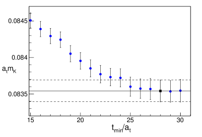
by setting the mass of the kaon to . This physical value was obtained in Ref. [24] by taking the isospin-symmetric limit and removing QED effects. We prefer scale setting with to the method of Ref. [23], which uses the mass of the Omega baryon (), due to difficulties in determining . Still, this scale should be viewed as indicative as the kaon mass was not extrapolated to the physical light quark masses but taken on this single ensemble only. However, our results for dimensionful quantities are naturally expressed in terms of so that the lattice spacing enters only in comparison with the literature in Fig. 7. The determination of , , and the renormalized anisotropy will be discussed shortly.
Although these 412 configurations are separated by Hybrid Monte Carlo (HMC) molecular dynamics trajectories of length , there is a small amount of residual autocorrelation evident in the measured correlation functions.222In lattice QCD the largest autocorrelations are typically observed for ‘smoothed’ observables such as the topological charge and smoothed action [25], which are not examined here. In order to mitigate effects of this autocorrelation on estimates of statistical uncertainties, we average measurements on pairs of subsequent configurations. Statistical errors are estimated using the bootstrap technique [26] on this rebinned ensemble with bootstrap samples.
In this anisotropic setup the lattice regulator is fully specified by the temporal lattice spacing and renormalized anisotropy . The anisotropy is determined from the (continuum) pion dispersion relation
| (2.3) |
where is the quantized finite-volume three-momentum of the pion.
Determination of requires the single-pion energies in Eq. 2.3. Periodic temporal boundary conditions are used for this ensemble, potentially complicating the extraction of finite-volume energies from the fall-off of temporal correlation functions. In particular, a single zero-momentum pion correlation function has the ‘cosh’ form in the limit of ground-state saturation
| (2.4) |
where is the relevant first excited-state energy. Two-pion correlation functions with zero total momentum have the more complicated form (ignoring small energy shifts due to pion interactions)
| (2.5) |
while two-pion correlation functions with non-zero total momenta have a similar but more complicated additional exponential term.
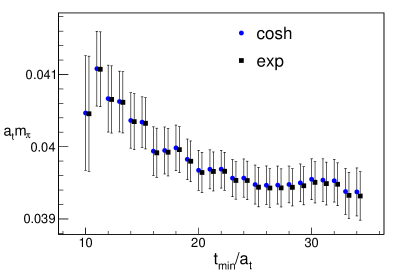
Since our finite-volume energies are extracted from fits of temporal correlation functions to an exponential form, these additional terms add potentially significant complication as has been discussed in (e.g.) Ref. [9]. Fortunately, the large temporal extent of our lattice () suppresses such terms below the statistical accuracy of the energy levels. This can be demonstrated by performing two-parameter correlated- fits of the single zero-momentum pion correlation function to both a single exponential and the cosh of Eq. 2.4. The second exponential in Eq. 2.4 is larger than or equal to the additional problematic exponential terms which appear in two-pion correlation functions, apart from small hadronic interaction effects.
As the single pion at rest is our most precisely determined correlation function, it is most sensitive to these thermal effects. The absence of these effects, such as the second exponential in Eq. 2.4, indicates that additional exponentials in two-pion correlation functions may be neglected. The comparison of single-exponential and cosh fits for various fitting ranges is shown in Fig. 1. Clearly, no effect from the finite temporal extent is evident for these temporal separations. All subsequent correlated- fits to temporal correlation functions will thus ignore finite- effects. The extraction of these energies will be discussed in more detail in Sec. 2.3.
The fits to the single-pion zero-momentum correlation function shown in Fig. 1, as well as all other fits to correlated data in this work, minimize a correlated- to properly treat the covariance between observables measured on the same ensemble of gauge configurations. The covariance matrix is obtained using the bootstrap estimator
| (2.6) |
where is the number of bootstrap samples, is the bootstrap replicum of on the th sample, and is the average over all bootstrap replica. The covariance matrix is taken as identical across each bootstrap sample’s determination of the fit parameters.
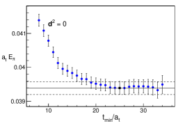
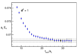
Apart from effects due to the finite temporal extent, the range of timeslices over which the fit is performed is another source of systematic error. In particular, fitted values exhibit a marked sensitivity to due to the influence of higher-lying exponentials in Eq. 1.1. In this work we employ ‘-plots’ to ensure that this systematic error is smaller than the statistical error on the fit parameters. The guidelines for selecting a satisfying this criterion are given in Eq. 2.13. These plots show the fitted values for many with a fixed , and are exemplified in Fig. 1 which shows -plots for and . With stochastically-estimated correlation functions, -plots are preferable to effective masses for determining the range of times over which a single exponential dominates. Stochastically-estimated effective masses typically have larger error than the corresponding fitted energies and are thus not useful to assess systematic errors from the choice of .
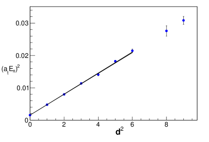
We now discuss two determinations of . In the first, single-pion energies at various total momenta333Pion correlation functions are averaged over equivalent momenta before fitting. are first obtained from this fitting procedure and then used in Eq. 2.3. The -plots for single-exponential fits to these correlation functions together with the fitted energies used in our analysis are given in Fig. 8 of App. A. Generally, these energies are chosen somewhat conservatively so that systematic errors due to excited-state contamination are small in comparison to the statistical errors. They are summarized in Fig. 2 together with a fit to Eq. 2.3 for . Correlation exists among the fitted energies; their covariance is estimated using the bootstrap method of Eq. 2.6 and fixed on each bootstrap sample. Evidently the continuum dispersion relation describes the single-pion energies up to large total momenta, suggesting that lattice spacing effects are under control here. The pion mass and determined from this linear fit (denoted ‘Strategy 1’) are given in Tab. 2.
An alternative determination (denoted ‘Strategy 2’) fits all single-pion correlation functions simultaneously to the ansatz
| (2.7) |
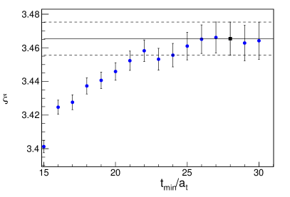
where the , and are free parameters. The covariance between all correlation functions at all time separations is explicitly taken into account in these correlated- fits. The results for from this fit are shown in Fig. 2 for various (identical for all correlation functions) together with the chosen fit range. This fit is also given in Tab. 2, where it is denoted ‘Strategy 2’.
Although the continuum dispersion relation fits the data well, we additionally perform fits like Strategy 2 but using the lattice-modified dispersion relation
| (2.8) |
The results of this fit are also consistent and shown in Tab. 2 as ‘Strategy 3’. For this work we take from Strategy 1 as it is the most conservative estimate, although the final results have little dependence on this choice.
| Strategy | |||
|---|---|---|---|
| 1 | 0.03938(19) | 3.451(11) | 1.4 |
| 2 | 0.03978(19) | 3.4654(98) | 1.19 |
| 3 | 0.03978(19) | 3.4649(98) | 1.20 |
2.2 Correlation function calculation
Because of the finite spatial extent and lattice spacing, the symmetry group of lattice QCD is , the double cubic point group. Irreducible representations of this group (or the relevant little group for a particular momentum) together with total isospin and -parity fully specify the quantum numbers of our energy eigenstates. Therefore, operators which transform irreducibly under these symmetries are employed. The procedure for constructing such operators is well known. Here we are concerned only with the ground state and low-lying excited states in the relevant irreducible representations (irreps). However, this work is part of a broader program to explore many higher-lying resonances in QCD. Interpolating operators with large overlap onto these higher-lying resonances are more complicated and require non-trivial spatial structures as in Refs. [16, 19]. Such operators are not used here, but rather only (smeared) single-site interpolators for each hadron.
Correlation matrices are typically required to obtain excited-state energies. In order to build correlation matrices in each of the irreps, we examine the expected non-interacting single- and two-pion levels. Generally, an interpolator for each of these levels below the inelastic threshold is included while additional two-pion operators are used as a check of systematic effects.
As discussed above, these multi-hadron correlation matrices require all-to-all quark propagators. We use the method of Ref. [11] which introduces noise in the subspace spanned by low-lying eigenmodes of the gauge-covariant Laplace operator. This noise can be diluted [12] in time (T), spin (S), and Laplacian eigenvector (L) indices, each of which can be fully diluted (‘F’) or have some number of dilution projectors ‘interlaced’ (‘I’) uniformly throughout the space. Note that the distillation method of Ref. [3] is recovered in the maximal dilution limit (TF, SF, LF).
| line type | scheme | ||||
|---|---|---|---|---|---|
| 264 | fixed | 5 | (TF, SF, LI8) | 8 | 1280 |
| relative | 2 | (TI16, SF, LI8) | - | 1024 |
On this anisotropic ensemble it is beneficial to choose different dilution schemes for quark propagators between different times (so-called ‘fixed’ quark lines) and for quark propagators starting and ending at the same time (‘relative’ quark lines). These different dilution schemes are specified in Tab. 3 together with the number of required Dirac matrix inversions () and low-lying Laplacian eigenvectors defining the LapH subspace (). In order to ensure an unbiased estimate of correlation functions, each quark line requires an independent stochastic source. The total number of such sources used per configuration () is shown in Tab. 3 together with the number of source times () used to reduce statistical errors. It should be noted that only fixed lines and relative lines (for a minimum ) are required to ensure unbiased estimates of the required correlation functions. However, additional source times and noise sources are employed here to increase statistics. While the additional noise sources are required for other systems, different noise combinations provide additional stochastic estimates and are thus averaged over. The required Wick contractions are enumerated in Ref. [11].
2.3 Finite-volume energies
After constructing the correlation functions as described in Sec. 2.2, the method for extracting finite-volume energies from them is now discussed. For this work we aim to utilize not only the ground state in each irreducible representation, but several excited states as well. In order to reliably extract these excited-state energies, solutions of a generalized eigenvalue problem are employed.
In each channel, a correlation matrix is formed consisting of a single-site interpolating operator (if present) together with the relevant two-pion operators. These two-pion operators are chosen to match the expected non-interacting states and all such operators below inelastic threshold are included.
For each of these correlation matrices () we solve the generalized eigenvalue problem
| (2.9) |
for a particular set of . The eigenvectors are used to define correlation functions between ‘optimal’ interpolators [27]
| (2.10) |
where the outer parentheses denote an inner product over GEVP indices. Although these optimal interpolators are constructed to have maximal overlap with a single Hamiltonian eigenstate, the off-diagonal elements of are not exactly zero resulting in a source of systematic error that must be assessed. It should be noted that this is a different approach to Refs. [28, 29] which require the solution of the GEVP at different , possibly introducing ambiguities between closely spaced levels at different times, but guaranteeing that the eigenvalues approach the desired exponential fall-off.
To extract energies in a particular channel we solve the GEVP of Eq. 2.9 and form the rotated correlation matrix of Eq. 2.10. The GEVP diagonalization is not performed on each bootstrap sample, due to similar ambiguities identifying closely spaced levels on different bootstrap samples. We first perform two-parameter correlated- fits with a single-exponential ansatz on the diagonal elements of the rotated correlation matrix to obtain a preliminary determination of the finite-volume spectra. These preliminary energies are used in Fig. 4 and with Eq. 3.20 to obtain a qualitative picture of the spectrum and nature of the states.
For our final analysis we employ a different approach which exploits the similarity (and correlation) between two-pion and single-pion correlation functions. As in Ref. [13] but here generalized to arbitrary momenta, for an optimized two-pion operator with pion momenta and (), we define the ratio
| (2.11) |
which is constructed on each bootstrap sample and fit in a fully correlated manner to the ansatz . The energy shift is used to reconstruct the desired energy via
| (2.12) |
where is obtained from the single-pion fits. In the channel, these two-hadron states mix with the -meson. For such mixed states these ratio fits are still beneficial, but exhibit an increased amount of excited-state contamination, which will be discussed shortly.
Several sources of systematic error in this procedure must be addressed. First, the fitting range is varied, in particular . Second, systematic errors due to the small but non-zero off-diagonal elements of must be assessed.
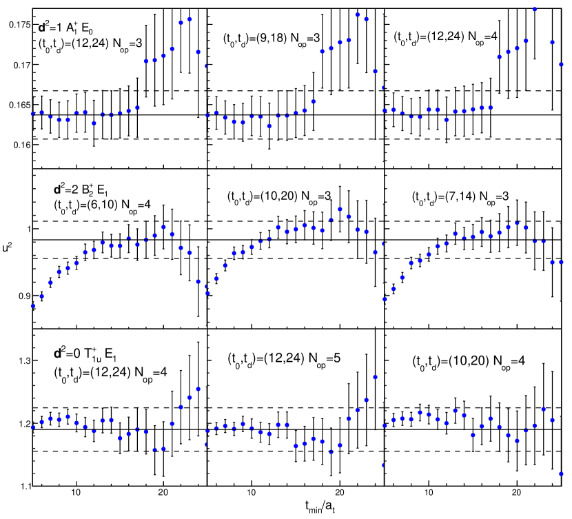
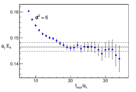
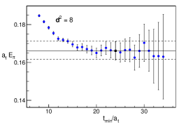
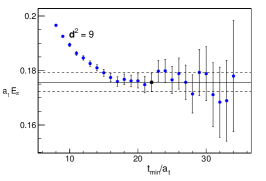
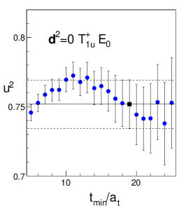
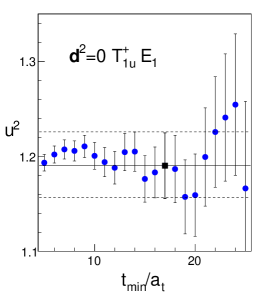
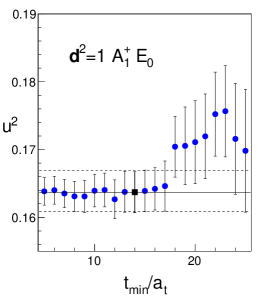
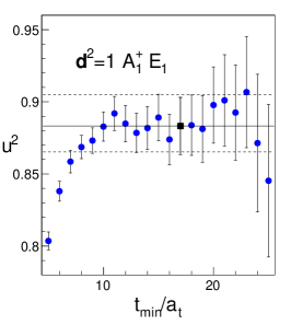
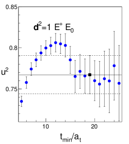
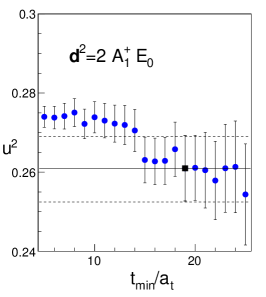
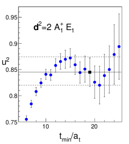
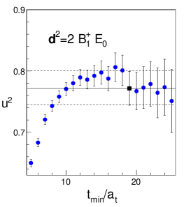
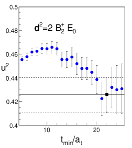
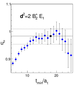
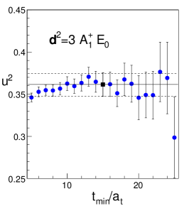
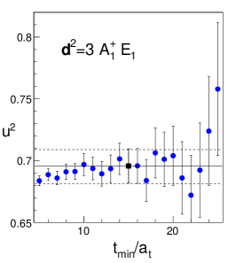
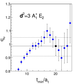
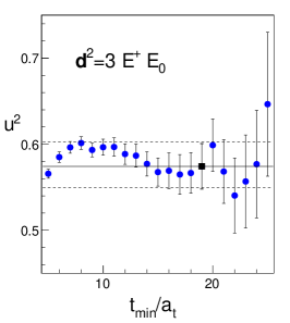
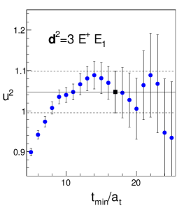
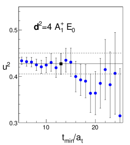
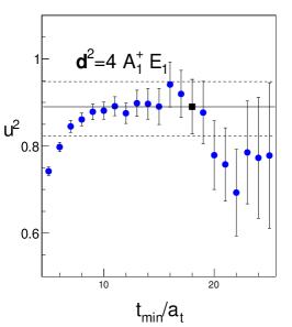
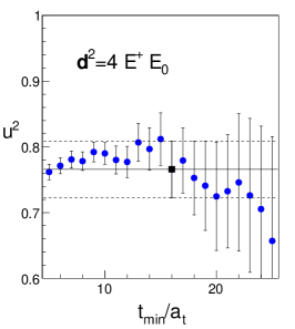
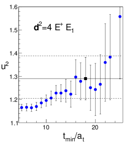
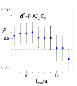
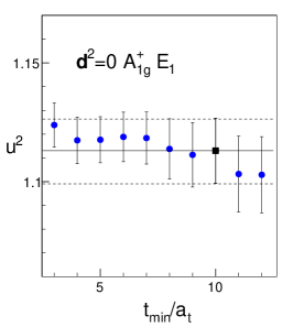
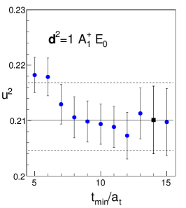
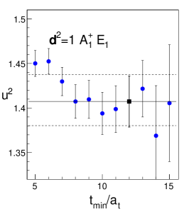
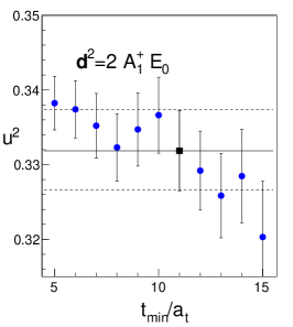
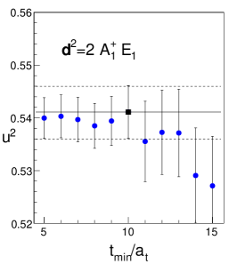
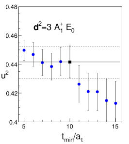
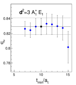
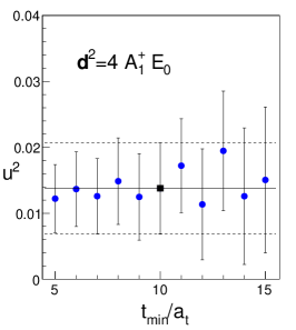
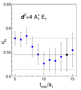
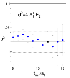
To this end, we not only vary the fitting range but also and the operators included in the GEVP. The variation of these systematics for a selection of energy levels is shown in Fig. 3. There the dimensionless center-of-mass momentum is shown, which is defined in Eq. 2.15.
Generally, systematic effects due to are the largest and must be treated with care. To this end we fix and choose conservatively. As minimum requirements we demand that the chosen gives a suitable correlated and that
| (2.13) |
where is the bootstrap error on and .
While these ratio fits have the advantage of directly determining the energy shifts, their excited-state contamination may have a non-standard form. This can be seen by examining the leading excited-state corrections for the ratio directly
| (2.14) |
where is the energy gap from the two-pion correlator in the numerator and the relevant interpolator-dependent prefactor, while and are the analogous quantities for each of the single-pion correlators in the denominator. If the first two excited states in the numerator effectively consist of one pion in the ground state and the other in an excited state, the overall excited-state contamination in will be very small. However, in general the excited-state contamination from the denominator enters with different sign, possibly causing a non-monotonically decreasing ‘bump’-type behavior in -plots. Such bumps must be taken into account when choosing fit ranges for the strongly-interacting states. Apart from Fig. 3, -plots for ratio fits performed to all correlation functions used in the phase shift analysis are shown in App. B and App. C. Although bumps are evident for some levels, we choose conservative fit ranges in those cases to ensure systematic effects from excited states are smaller than the statistical error.
2.4 Scattering phase shifts
After discussing the procedure for extracting finite-volume energies, we now turn to using them to calculate elastic scattering phase shifts. The relation between finite-volume energy spectra and infinite-volume elastic scattering amplitudes is derived in Ref. [2] and generalized to non-zero total momentum in Ref. [30]. A useful summary of the method for several different situations may be found in Ref. [31], while generalizations to asymmetric spatial volumes [32], multiple coupled two-particle channels [33] and three-particle scattering [34, 35, 36] have been developed.
For scattering between two identical particles of mass , we denote by the energy measured in the lattice (‘lab’) frame in a particular irrep with total momentum . We define the kinematical variables
| (2.15) |
Up to exponentially suppressed finite-volume effects, the elastic scattering matrix is related to the finite-volume energy spectra via the well-known quantization condition, which is a matrix equation of the form
| (2.16) |
where is the infinite-volume scattering matrix and the determinant is taken over the indices corresponding to total angular momentum, its projection along some axis, orbital angular momentum, and spin, respectively. Note that the matrix in general mixes different partial waves.
For elastic scattering between identical spin-zero particles and . In this case the matrix is given by
| (2.17) | ||||
| (2.18) |
where and are summed over and we have introduced the Lüscher zeta functions . We use a representation of the zeta functions given in App. A of Ref. [31] for their numerical evaluation, which is consistent with an independent implementation based on an alternative representation discussed in Ref. [20].
While we have expressed in the basis, it is more convenient to express the relation in terms of finite-volume irreps, as both and become block diagonal, facilitating the evaluation of the determinant.
| irrep | |||
| 0 | |||
| 1 | |||
After performing this block diagonalization and neglecting the contribution of higher partial waves, the relationship between the scattering phase shifts and
| (2.19) |
for each irrep is shown in Tab. 4. One advantage of employing expressions relating the real part of the inverse scattering amplitude to the is that the analyticity of near threshold is explicit. For weakly interacting channels such as the , this enables a smooth behavior between positive and negative . As we treat identical-particle scattering, particle-exchange symmetry prevents mixing between successive partial waves in moving frames. Neglecting the remaining partial wave mixing amounts to neglecting the , and , partial waves.
3 Results
This section contains our results for elastic scattering phase shifts. We neglect exponential finite-volume corrections and, as discussed in Sec. 2.4, treat only the lowest partial wave which contributes to each lattice irrep. Our results are interpreted in terms of the effective range expansion, which provides the correct threshold behavior of the scattering amplitude while also accommodating resonances. Finite-volume energy levels near or above the inelastic threshold are not described by the elastic Lüscher formulae of Sec. 2.4 and thus not used.
3.1
The , partial wave contains the -resonance. Not only is this evident in the scattering phase shifts, but it is also suggested by examining the overlaps of interpolating operators onto finite-volume Hamiltonian eigenstates. Specifically, we estimate by forming the ratio
| (3.20) |
where is the fitted energy, and taking . For each interpolating operator the overlaps onto the Hamiltonian eigenstates are plotted in Fig. 4 together with the
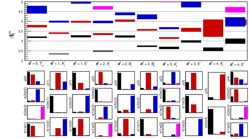
energies extracted from single-exponential fits. Center-of-mass energies are shown in that figure to facilitate comparison between channels with different total momenta.
As expected, local -meson interpolating operators have significant overlap with energy eigenstates near the resonance mass , where mixing with two-pion operators can be observed. However, only two-pion interpolating operators have significant overlap with energy eigenstates outside this resonance region. For states which have significant overlap onto two-pion interpolators only, the ratio fits described previously have very little excited state contamination. Clearly, there are a number of states near or above the four-pion threshold . While these states can be extracted with suitable statistical precision, their interpretation in terms of infinite-volume scattering amplitudes is unknown.
| irrep | level | |||||||
| 0 | 19 | 1.18 | -0.01214(91) | 3.206(25) | 2.05(29) | |||
| 1 | 17 | 0.84 | 0.0086(15) | 3.734(40) | -5.1(1.1) | |||
| 0 | 14 | 1.22 | -0.00106(18) | 2.3168(61) | 7.9(1.5) | |||
| 1 | 17 | 0.99 | -0.01429(89) | 3.373(27) | 0.34(17) | |||
| 0 | 19 | 0.9 | -0.0196(11) | 3.226(34) | 1.28(21) | |||
| 0 | 19 | 0.84 | -0.00225(42) | 2.486(15) | 4.8(1.1) | |||
| 1 | 19 | 1.2 | -0.0216(12) | 3.325(36) | -1.05(12) | |||
| 0 | 19 | 0.83 | -0.0248(12) | 3.232(37) | 0.90(19) | |||
| 0 | 22 | 1.0 | -0.00351(72) | 2.749(24) | 3.8(1.1) | |||
| 1 | 18 | 1.07 | 0.0210(11) | 3.495(34) | -1.08(18) | |||
| 0 | 15 | 1.33 | -0.00199(63) | 2.650(22) | 6.6(2.6) | |||
| 1 | 15 | 1.39 | -0.00091(56) | 3.132(22) | 2.3(3.4) | |||
| 2 | 20 | 1.67 | -0.0330(27) | 3.498(85) | -2.10(39) | |||
| 0 | 19 | 1.07 | -0.0060(11) | 2.966(38) | 3.22(98) | |||
| 1 | 17 | 1.07 | 0.0129(20) | 3.570(62) | -3.61(48) | |||
| 0 | 13 | 0.99 | -0.00269(92) | 2.751(35) | 5.2(2.5) | |||
| 1 | 18 | 1.06 | 0.0154(23) | 3.382(79) | -1.78(40) | |||
| 0 | 16 | 1.03 | 0.0107(16) | 3.225(58) | 1.89(67) | |||
| 1 | 18 | 1.31 | 0.0296(32) | 3.84(10) | -0.1(2.3) |
Numerical results for our final analysis using ratio fits are listed in Tab. 5, where is obtained by applying the formulae of Tab. 4.
This particular quantity is the real part of the inverse scattering amplitude and is thus analytic in the complex momentum plane near the two-pion threshold , making it a natural choice for fits of the amplitude’s energy dependence.
For this resonant partial wave, can be described by the Breit-Wigner parametrization
| (3.21) |
which also has the correct threshold behavior dictated by the effective range expansion. A two-parameter (fully-correlated) -fit to Eq. 3.21 is performed. This fit must not only take into account the correlation between different data points, but also the correlation between and for each data point. In order to do this, we employ the correlated- which is the maximum likelihood estimator for the distribution of the residuals
| (3.22) | ||||
As with the other fits in this work, the bootstrap estimator is used to estimate the covariance between the . However, each depends nontrivially on the fit parameters and so the bootstrap estimate of the covariance must be recalculated on each call to the correlated- function. In other words, on each bootstrap sample, each call to the correlated- employs all bootstrap samples to estimate the covariance. While this method may seem cumbersome, it ensures that all correlations among the data are taken into account.
The results of this fit are
| (3.23) |
While other resonance parametrizations have been applied (in e.g. Ref. [8]) which maintain unitarity above the resonance region, given the proximity of the four-pion threshold such parametrizations seem poorly motivated here. However, we test the dependence of these resonance parameters on the Breit-Wigner fit form by employing a non-relativistic ansatz to
| (3.24) |
where is an energy-independent width and parametrizes a slowly-varying background. This three-parameter fit gives
| (3.25) |
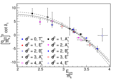
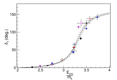
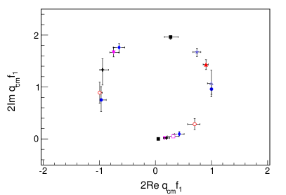
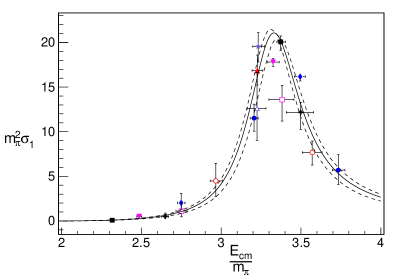
A summary of our data as well as the fit of Eq. 3.23 are shown in Fig. 5. Several different representations of the data are shown in that figure. First, the data points are shown with the corresponding fit to them. Then, is shown (in ) with the fit to . The rapid variation of the phase shift is clear in this plot. Further evidence of this rapid variation is seen in an Argand plot showing the real and imaginary parts of the partial wave amplitude (following the conventions of Ref. [37])
| (3.26) |
Finally, a plot of the partial wave cross section
| (3.27) |
shows a clear enhancement due to the resonance.
Due to the singular nature of the Lüscher zeta functions at non-interacting energies, the distribution of bootstrap samples of the quantities shown in Fig. 5 can show significant asymmetry. In that figure we therefore display asymmetric bootstrap error bars. Displaying the points in this manner indicates the level of asymmetry but ignores the correlation between the horizontal and vertical error bars.
3.2
| irrep | level | |||||||
| 0 | 9 | 1.4 | 0.00082(17) | 0.0210(42) | -16.5(3.2) | |||
| 1 | 10 | 1.16 | 0.00519(63) | 2.324(40) | -7.9(1.1) | |||
| 0 | 14 | 0.97 | 0.00170(35) | 0.439(12) | -10.8(2.1) | |||
| 1 | 12 | 1.07 | 0.0075(11) | 2.939(66) | -5.6(1.1) | |||
| 0 | 11 | 1.24 | 0.00133(26) | 0.693(12) | -10.3(2.2) | |||
| 1 | 10 | 1.14 | 0.00191(23) | 1.130(16) | -7.81(84) | |||
| 0 | 10 | 1.43 | 0.00158(48) | 0.922(24) | -6.9(2.9) | |||
| 1 | 10 | 1.05 | 0.00447(44) | 1.732(31) | -8.01(72) | |||
| 0 | 10 | 1.13 | 0.00089(33) | 0.029(14) | -7.3(3.9) | |||
| 1 | 14 | 1.27 | 0.0057(19) | 1.137(67) | -5.7(4.1) | |||
| 2 | 12 | 1.23 | 0.00017(68) | 2.131(51) | -23(31) |
The channel is weakly interacting and thus a good test of the stochastic LapH method. As in the case, we examine the real part of the inverse scattering amplitude, which is analytic near the two-pion threshold. Our fitted energies and resultant phase shifts for the partial wave are shown in Tab. 6.
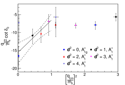
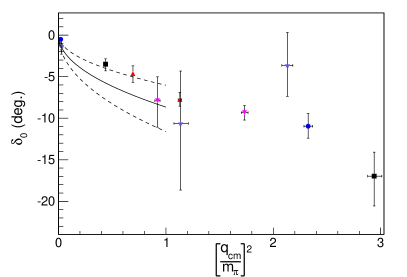
The weakly interacting nature of this channel motivates its description by the lowest few terms of the effective range expansion
| (3.28) |
This parametrization is expected to be valid for momenta below the -channel cut [38].
Our results are collected in Fig. 6. Due to the smaller number of finite-volume irreps in which the partial wave appears, there are only four points in this low-momentum region. A two-parameter fit to the effective range ansatz of Eq. 3.28 yields
| (3.29) |
The small number of points in this channel suggests that not much can be gained by adding the next term in the effective range expansion which contains the shape parameter. The scattering length is determined with about precision and is consistent with the (continuum) PT extrapolation of (e.g.) Ref. [13] but the pion mass used in this work is lighter than those employed there.
4 Conclusions
The elastic and scattering phase shifts are determined from a dynamical lattice QCD simulation in a large spatial volume with a light pion mass. In particular, the stochastic estimation scheme employed here performs efficiently, and determines the correlation functions with sufficient precision to extract the finite-volume energies and scattering phase shifts. This suggests that larger volumes and lighter pions are possible due to the favorable scaling of the stochastic LapH method.
After extracting finite-volume energy levels, the Lüscher method is employed to calculate elastic scattering phase shifts. The , partial wave is well described by a Breit-Wigner form and exhibits rapid phase motion indicative of a resonance. Our main results are Fig. 5 and Eq. 3.23. We have compiled recent published calculations of the -resonance in Fig. 7
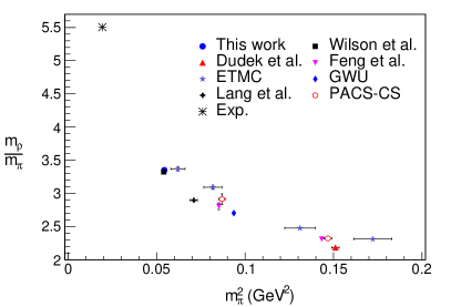
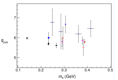
indicating that this calculation (together with Ref. [22]) is the closest to the physical quark masses achieved so far. Fig. 7 compares to reduce scale uncertainties, as none of the results are extrapolated to the continuum limit. The results for the mass are generally in good agreement, but is known with considerably less precision.
Due to our light quark masses, the lowest inelastic threshold (due to four pions) is close to the resonance region limiting the applicability of the elastic Lüscher formulae. Hopefully, existing work on extending the Lüscher formulae to three-particle scattering [34, 35, 36] can be adapted to treat these thresholds in the future. Of course, the problem worsens as the quark masses are lowered to their physical values as experimentally . Once this threshold can be treated quantitatively its effect may be small, as the experimental branching fraction for is below the percent level.
We have less points below inelastic threshold for the , partial wave, as there are fewer lattice irreps in which it appears. Still, our data below the -channel cut is well-described by the first two terms in the effective range expansion and provides a determination of the scattering length to about 20%. Our results for are shown in Fig. 6 and Eq. 3.29. Calculations of the -wave scattering length444For a recent review of these calculations see Ref. [13] and the references quoted therein. are considerably more advanced than in , so a single-ensemble result is not fit for direct comparison. However, the error on is somewhat remarkable given our stochastic estimation of the all-to-all quark propagators and the precise calculation of small energy shifts required to obtain a signal.
As mentioned in the introduction, Ref. [22] appeared during the preparation of this manuscript which uses the full distillation method to treat the required all-to-all propagators and can be viewed as the maximal dilution limit of our approach. We compare results in Tab. 7 for a selection of published
| Ref. | ||||||
|---|---|---|---|---|---|---|
| This work | 2304 | 0.03939(19) | 0.12625(94) | 0.1470(16) | 0.13190(87) | 5.99(26) |
| Ref. [22] | 393216 | 0.03928(18) | 0.12488(40) | 0.14534(52) | 0.13175(35) | 5.688(70) |
numbers as well as the required number of Dirac matrix inversions per configuration. Although and are also obtained in Ref. [22] from a Breit-Wigner ansatz, their fitting method constructs a correlated- directly from the finite-volume energies rather than . However, the errors on and (which are comparable to those on the energies) are not taken into account in their fit procedure. It is unclear what effect this has on the resultant fit parameters and their errors. Our methods for extracting finite-volume energies are also different from those employed in Ref. [22].
We see that the distillation results are comparable in precision for the pion, but have roughly half the statistical error for two-pion states, while requiring about 170 times more Dirac matrix inversions per configuration. The Dirac matrix inversion cost for the distillation method is significantly larger than the cost for the gauge generation and does not include the (sizeable) cost of constructing correlation functions from the sources and solutions, which also scales poorly with the volume. Even so, presumably a 170-fold increase in computational effort would reduce the error on our results by more than an order of magnitude, making them significantly more precise than Ref. [22].
Overall, this first large-volume scattering calculation using stochastic LapH is promising for future work. As it is clear that scattering calculations are entering a new era of increased statistical precision, it is important to quantify the remaining systematic errors. These include exponential finite-volume effects, the effect of higher partial waves, the presence of inelastic thresholds, and lattice spacing effects. To this end, work has progressed [21] in applying the stochastic LapH method to state-of-the-art ensembles generated by the Coordinate Lattice Simulations (CLS) consortium [43]. Apart from the elastic scattering phase shifts presented here, these isotropic ensembles simplify the renormalization and -improvement pattern of composite operators, enabling the determination of resonance matrix elements. Preliminary work on the simplest such matrix element, the timelike pion form factor, is also reported in Ref. [21]. Finally, pushing to lighter pions would be desired. While this can be done using these CLS ensembles, the lower inelastic thresholds limit the applicability of the Lüscher formula. More theoretical work is required to rigorously treat these thresholds.
Acknowledgements: We acknowledge helpful conversations with Robert Edwards, David Wilson, and Max Hansen. BH is supported by Science Foundation Ireland under Grant No. 11/RFP/PHY3218. CJM acknowledges support from the U.S. NSF under award PHY-1306805 and through TeraGrid/XSEDE resources provided by TACC, SDSC, and NICS under grant number TG-MCA07S017. The USQCD QDP++ library [44] and the Improved BiCGStab solver in Chroma were used in developing the software for early stages of the calculations reported here.
Appendix A -plots for moving pions
All -plots for fits to single-pion correlation functions at various momenta are shown in Fig. 8. These energies are used in Strategy 1 discussed in Sec. 2.1 to determine the renormalized anisotropy .
Appendix B -plots for all levels
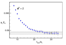
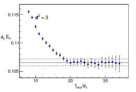
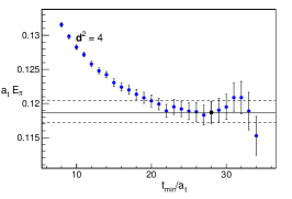
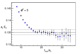
All -plots for finite volume energies used in the determination of the , elastic scattering amplitude are shown in Figs. 9, 10, 11, 12, and 13. The ratio fits of Eq. 2.11 are employed and the dimensionless center-of-mass momentum is shown.
Appendix C -plots for all levels
As in App. B, this appendix contains -plots for all finite volume energies used in the determination of the , scattering amplitude. They are shown in Figs. 14, 15, 16, and 17.
References
- [1] L. Maiani and M. Testa, Final state interactions from Euclidean correlation functions, Phys. Lett. B245 (1990) 585–590.
- [2] M. Lüscher, Two particle states on a torus and their relation to the scattering matrix, Nucl. Phys. B354 (1991) 531–578.
- [3] Hadron Spectrum Collaboration, M. Peardon, J. Bulava, J. Foley, C. Morningstar, J. Dudek, R. G. Edwards, B. Joo, H.-W. Lin, D. G. Richards, and K. J. Juge, A Novel quark-field creation operator construction for hadronic physics in lattice QCD, Phys. Rev. D80 (2009) 054506, [arXiv:0905.2160].
- [4] D. J. Wilson, J. J. Dudek, R. G. Edwards, and C. E. Thomas, Resonances in coupled scattering from lattice QCD, Phys. Rev. D91 (2015), no. 5 054008, [arXiv:1411.2004].
- [5] C. B. Lang, L. Leskovec, D. Mohler, S. Prelovsek, and R. M. Woloshyn, mesons with and scattering near threshold, Phys. Rev. D90 (2014), no. 3 034510, [arXiv:1403.8103].
- [6] S. Prelovsek, L. Leskovec, C. Lang, and D. Mohler, K scattering and the K* decay width from lattice QCD, Phys.Rev. D88 (2013), no. 5 054508, [arXiv:1307.0736].
- [7] C. B. Lang, D. Mohler, S. Prelovsek, and M. Vidmar, Coupled channel analysis of the rho meson decay in lattice QCD, Phys. Rev. D84 (2011), no. 5 054503, [arXiv:1105.5636]. [Erratum: Phys. Rev.D89,no.5,059903(2014)].
- [8] Hadron Spectrum Collaboration, J. J. Dudek, R. G. Edwards, and C. E. Thomas, Energy dependence of the resonance in elastic scattering from lattice QCD, Phys.Rev. D87 (2013), no. 3 034505, [arXiv:1212.0830].
- [9] J. J. Dudek, R. G. Edwards, and C. E. Thomas, S and D-wave phase shifts in isospin-2 pi pi scattering from lattice QCD, Phys. Rev. D86 (2012) 034031, [arXiv:1203.6041].
- [10] C. Lang and V. Verduci, Scattering in the negative parity channel in lattice QCD, Phys.Rev. D87 (2013), no. 5 054502, [arXiv:1212.5055].
- [11] C. Morningstar, J. Bulava, J. Foley, K. J. Juge, D. Lenkner, M. Peardon, and C. H. Wong, Improved stochastic estimation of quark propagation with Laplacian Heaviside smearing in lattice QCD, Phys. Rev. D83 (2011) 114505, [arXiv:1104.3870].
- [12] J. Foley, K. Jimmy Juge, A. O’Cais, M. Peardon, S. M. Ryan, and J.-I. Skullerud, Practical all-to-all propagators for lattice QCD, Comput. Phys. Commun. 172 (2005) 145–162, [hep-lat/0505023].
- [13] ETM Collaboration, C. Helmes, C. Jost, B. Knippschild, C. Liu, J. Liu, L. Liu, C. Urbach, M. Ueding, Z. Wang, and M. Werner, Hadron-hadron interactions from Nf = 2 + 1 + 1 lattice QCD: isospin-2 scattering length, JHEP 09 (2015) 109, [arXiv:1506.0040].
- [14] C. Hanhart, J. R. Pelaez, and G. Rios, Remarks on pole trajectories for resonances, Phys. Lett. B739 (2014) 375–382, [arXiv:1407.7452].
- [15] D. R. Bolton, R. A. Briceno, and D. J. Wilson, Connecting physical resonant amplitudes and lattice QCD, Phys. Lett. B757 (2016) 50–56, [arXiv:1507.0792].
- [16] S. Basak, R. G. Edwards, G. T. Fleming, U. M. Heller, C. Morningstar, D. Richards, I. Sato, and S. Wallace, Group-theoretical construction of extended baryon operators in lattice QCD, Phys. Rev. D72 (2005) 094506, [hep-lat/0506029].
- [17] J. M. Bulava et al., Excited State Nucleon Spectrum with Two Flavors of Dynamical Fermions, Phys. Rev. D79 (2009) 034505, [arXiv:0901.0027].
- [18] J. Bulava, R. G. Edwards, E. Engelson, B. Joo, H.-W. Lin, C. Morningstar, D. G. Richards, and S. J. Wallace, Nucleon, and excited states in lattice QCD, Phys. Rev. D82 (2010) 014507, [arXiv:1004.5072].
- [19] C. Morningstar, J. Bulava, B. Fahy, J. Foley, Y. Jhang, et al., Extended hadron and two-hadron operators of definite momentum for spectrum calculations in lattice QCD, Phys.Rev. D88 (2013), no. 1 014511, [arXiv:1303.6816].
- [20] B. Fahy, J. Bulava, B. Hörz, K. J. Juge, C. Morningstar, and C. H. Wong, Pion-pion scattering phase shifts with the stochastic LapH method, PoS LATTICE2014 (2015) 077, [arXiv:1410.8843].
- [21] J. Bulava, B. Hörz, B. Fahy, K. J. Juge, C. Morningstar, and C. H. Wong, Pion-pion scattering and the timelike pion form factor from lattice QCD simulations using the stochastic LapH method, in Proceedings, 33rd International Symposium on Lattice Field Theory (Lattice 2015), 2015. arXiv:1511.0235.
- [22] D. J. Wilson, R. A. Briceno, J. J. Dudek, R. G. Edwards, and C. E. Thomas, Coupled scattering in -wave and the resonance from lattice QCD, Phys. Rev. D92 (2015), no. 9 094502, [arXiv:1507.0259].
- [23] Hadron Spectrum Collaboration, H.-W. Lin et al., First results from 2+1 dynamical quark flavors on an anisotropic lattice: Light-hadron spectroscopy and setting the strange-quark mass, Phys. Rev. D79 (2009) 034502, [arXiv:0810.3588].
- [24] G. Colangelo et al., Review of lattice results concerning low energy particle physics, Eur. Phys. J. C71 (2011) 1695, [arXiv:1011.4408].
- [25] ALPHA Collaboration, S. Schaefer, R. Sommer, and F. Virotta, Critical slowing down and error analysis in lattice QCD simulations, Nucl. Phys. B845 (2011) 93–119, [arXiv:1009.5228].
- [26] B. Efron and R. Tibshirani, Bootstrap methods for standard errors, confidence intervals, and other measures of statistical accuracy, Statist. Sci. 1 (02, 1986) 54–75.
- [27] C. Michael and I. Teasdale, Extracting Glueball Masses From Lattice QCD, Nucl. Phys. B215 (1983) 433.
- [28] M. Luscher and U. Wolff, How to Calculate the Elastic Scattering Matrix in Two-dimensional Quantum Field Theories by Numerical Simulation, Nucl. Phys. B339 (1990) 222–252.
- [29] B. Blossier, M. Della Morte, G. von Hippel, T. Mendes, and R. Sommer, On the generalized eigenvalue method for energies and matrix elements in lattice field theory, JHEP 04 (2009) 094, [arXiv:0902.1265].
- [30] K. Rummukainen and S. A. Gottlieb, Resonance scattering phase shifts on a nonrest frame lattice, Nucl. Phys. B450 (1995) 397–436, [hep-lat/9503028].
- [31] M. Gockeler, R. Horsley, M. Lage, U. G. Meissner, P. E. L. Rakow, A. Rusetsky, G. Schierholz, and J. M. Zanotti, Scattering phases for meson and baryon resonances on general moving-frame lattices, Phys. Rev. D86 (2012) 094513, [arXiv:1206.4141].
- [32] X. Feng, X. Li, and C. Liu, Two particle states in an asymmetric box and the elastic scattering phases, Phys. Rev. D70 (2004) 014505, [hep-lat/0404001].
- [33] S. He, X. Feng, and C. Liu, Two particle states and the S-matrix elements in multi-channel scattering, JHEP 07 (2005) 011, [hep-lat/0504019].
- [34] K. Polejaeva and A. Rusetsky, Three particles in a finite volume, Eur. Phys. J. A48 (2012) 67, [arXiv:1203.1241].
- [35] M. T. Hansen and S. R. Sharpe, Relativistic, model-independent, three-particle quantization condition, Phys. Rev. D90 (2014), no. 11 116003, [arXiv:1408.5933].
- [36] M. T. Hansen and S. R. Sharpe, Expressing the three-particle finite-volume spectrum in terms of the three-to-three scattering amplitude, Phys. Rev. D92 (2015), no. 11 114509, [arXiv:1504.0424].
- [37] J. Taylor, Scattering Theory: The Quantum Theory of Nonrelativistic Collisions. Dover Books on Engineering. Dover Publications, 2012.
- [38] NPLQCD Collaboration, S. R. Beane, E. Chang, W. Detmold, H. W. Lin, T. C. Luu, K. Orginos, A. Parreno, M. J. Savage, A. Torok, and A. Walker-Loud, The I=2 pipi S-wave Scattering Phase Shift from Lattice QCD, Phys. Rev. D85 (2012) 034505, [arXiv:1107.5023].
- [39] X. Feng, K. Jansen, and D. B. Renner, Resonance Parameters of the rho-Meson from Lattice QCD, Phys. Rev. D83 (2011) 094505, [arXiv:1011.5288].
- [40] X. Feng, S. Aoki, S. Hashimoto, and T. Kaneko, Timelike pion form factor in lattice QCD, Phys. Rev. D91 (2015), no. 5 054504, [arXiv:1412.6319].
- [41] C. Pelissier and A. Alexandru, Resonance parameters of the rho-meson from asymmetrical lattices, Phys. Rev. D87 (2013), no. 1 014503, [arXiv:1211.0092].
- [42] CS Collaboration, S. Aoki et al., Meson Decay in 2+1 Flavor Lattice QCD, Phys. Rev. D84 (2011) 094505, [arXiv:1106.5365].
- [43] M. Bruno et al., Simulation of QCD with N 2 1 flavors of non-perturbatively improved Wilson fermions, JHEP 02 (2015) 043, [arXiv:1411.3982].
- [44] SciDAC Collaboration, R. G. Edwards and B. Joo, The Chroma software system for lattice QCD, Nucl. Phys. Proc. Suppl. 140 (2005) 832.