Interior eigenvalue density of large bi-diagonal matrices subject to random perturbations

Abstract.

We study the spectrum of large a bi-diagonal Toeplitz matrix subject to a Gaussian random perturbation with a small coupling constant. We obtain a precise asymptotic description of the average density of eigenvalues in the interior of the convex hull of the range symbol.

Résumé. Nous étudions le spectre d’une grande matrice de Toeplitz soumise à une perturbation gaussienne avec petite constante de couplage. Nous obtenons une description asymptotique précise de la densité moyenne des valeurs propres à l’intérieur l’enveloppe convexe de l’image du symbole.

1. Introduction and main result

It is well known that the spectrum of non-normal operators can be extremely unstable even under tiny perturbations, see e.g. [7, 5]. It is therefore a natural question to study the spectra of such operators subject to small random perturbations. Recently, there has been a mounting interest in the spectral properties of elliptic non-normal (pseudo-)differential operators with small random perturbations, see for example [2, 10, 12, 17, 22, 4]. An interesting, perhaps surprising, result is that by adding a small random perturbation, we can obtain a probabilistic Weyl law for the eigenvalues for a large class of such operators.

Another important example is the case of non-normal Toeplitz matrices, since they can arise for example in models non-hermitian quantum mechanics, see e.g. [8, 13]. The authors’ interest in this case, however, is motivated by the aspect of spectral instability.

The goal of this work is to study the spectrum of random perturbations of the following bidiagonal $N\times N$ Toeplitz matrix:

(1.1) $$P=\begin{pmatrix}0&a&0&..&..&0\\ b&0&a&..&..&0\\ 0&b&0&..&..&0\\ ..&..&..&..&..&..\\ 0&..&..&..&0&a\\ 0&0&..&..&b&0\end{pmatrix}.$$

Here $a,\,b\in{\bf C}\setminus\{0\}$ and $N\gg 1$. Identifying ${\bf C}^{N}$ with $\ell^{2}([1,N])$, $[1,N]=\{1,2,..,N\}$ and also with $\ell^{2}_{[1,N]}({\bf Z})$ (the space of all $u\in\ell^{2}({\bf Z})$ with support in $[1,N]$), we have:

(1.2) $$P=1_{[1,N]}(a\tau_{-1}+b\tau_{1})1_{[1,N]}=1_{[1,N]}(a\mathrm{e}^{iD_{x}}+b\mathrm{e}^{-iD_{x}})1_{[1,N]},$$

where $\tau_{k}u(j)=u(j-k)$ denotes translation by $k$, and

$$(a\mathrm{e}^{iD_{x}}+b\mathrm{e}^{-iD_{x}})u(n)=\frac{1}{2\pi}\int_{\mathbf{R}/2\pi\mathbf{Z}}\mathrm{e}^{in\xi}p(\xi)\widehat{u}(\xi)d\xi,\quad u\in\ell^{2}(\mathbf{Z}),$$

where $\widehat{u}$ denotes the Fourier transformation of $u$ and $p(\xi)$ is the symbol of $P$, given by

(1.3) $$p(\xi)=a\mathrm{e}^{i\xi}+b\mathrm{e}^{-i\xi}.$$

Assume, to fix the ideas, that $|b|\leq|a|$. Then $p({\bf R})$ is equal to the ellipse, $E_{1}$, centred at 0 with major semi-axis of length $(|a|+|b|)$ pointing in the direction $e^{i(\alpha+\beta)/2}$, where $\alpha=\mathrm{arg}(a)$, $\beta=\mathrm{arg}(b)$, and minor semi-axis of length $|a|-|b|$. The focal points of $E_{1}$ are

(1.4) $$\pm 2\sqrt{ab}=\pm e^{i\frac{\alpha+\beta}{2}}2\sqrt{|a||b|}.$$

In a previous work [19] the authors have shown that the numerical range of $P$ is contained in the convex hull of the ellipse $E_{1}$ described above and the eigenvalues of $P$ are given by

(1.5) $$z=z(\nu)=2\sqrt{ab}\cos\left(\frac{\pi\nu}{N+1}\right),\quad\nu=1,\dots,N.$$

This result is also illustrated in Figure 1. In this work, we consider the following random perturbation of $P$

(1.6) $$P_{\delta}:=P+\delta Q_{\omega},\quad Q_{\omega}=(q_{j,k}(\omega))_{1\leq j,k\leq N},$$

where $0\leq\delta\ll 1$, possibly depending on $N$, and $q_{j,k}(\omega)$ are independent and identically distributed complex Gaussian random variables, following the complex Gaussian law $\mathcal{N}_{\mathbf{C}}(0,1)$.

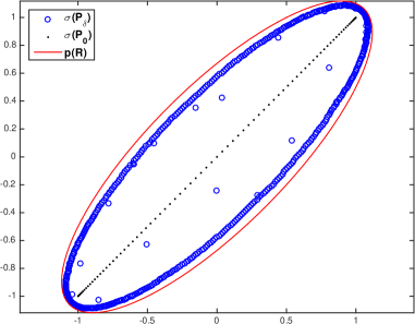
Figure 1. The black dots along the focal segment show the spectrum (obtained using MATLAB) of the unperturbed operator $P$ with dimension $N=501$, $a=0.5$, $b=i$ and $\delta=10^{-12}$. The blue cirlces show the spectrum of the perturbed operator (1.6), and the red ellipse is the image of the symbol $p$.

In [19], the authors proved that when the coupling constant $\delta$ is bounded from above and from below by sufficiently negative powers of $N$, then most eigenvalues of $P_{\delta}$, (1.6), are close to the ellipse $p(\mathbf{R})$ and follow a Weyl law, with probability close to one, as the dimension $N$ gets large (cf. Figure 1).

The methods used in [19] are essentially based on probabilistic subharmonic estimates of $\ln|\det(P_{\delta}-z)|$ and complex analysis, using in particular a counting theorem of [20] (see also [11, 12]). However, this approach is not fine to enough give a detailed description of the exceptional eigenvalues seen inside the ellipse in Figure 1 and we only obtain a logarithmic upper bound on the number of eigenvalues in this region. To gain more information about these eigenvalues, we study the random measure

(1.7) $$\Xi:=\sum_{z\in\sigma(P_{\delta})}\delta_{z},$$

where the eigenvalues are counted with multiplicity. In particular we are interested in studying the first intensity measure of $\Xi$, which is the positive measure $\nu$ defined by

(1.8) $$\mathds{E}\left[\Xi(\varphi)\right]=\int\varphi(z)\nu(dz),$$

where $\varphi$ is a test function of class $\mathcal{C}_{0}$. The measure $\nu$ contains information about the average density of eigenvalues, and we will show in Theorem 1.1 below, that it admits a continuous density with respect to the Lebesgue measure on $\mathbf{C}$, up to a small error in the large $N$ limit.

This approach is more classical in the theory of random polynomials (cf. [15, 1]) and random Gaussian analytic functions (cf. [14, 21]). We follow in particular the approach developed in [22], which was therein used to describe the average density of eigenvalues of a class of semiclassical differential operators subject to small random perturbations.

The main result of this paper describes the average density of eigenvalues in the interior of confocal ellipses. Let $p_{a,b}=p$ as in (1.3). For any $r>0$ we define $\Sigma_{r}$ to be the convex hull of $p_{ra,r^{-1}b}(\mathbf{R})$. We will see in Section 2 that $p_{ra,r^{-1}b}(\mathbf{R})$, for $(|b|/|a|)^{1/2}\leq r<+\infty$, are confocal ellipses and that they are in the interior of $\Sigma_{r_{0}}$, for every $r_{0}>r$. Moreover that $p_{ra,r^{-1}b}(\mathbf{R})$, with $r=(|b|/|a|)^{1/2}$, is the focal segment.

We prove the following result.

Theorem 1.1.

Let $P_{\delta}$ be as in (1.6) and let $p_{a,b}=p$ as in (1.3). Let $C\gg 1$ be arbitrary, but fixed (and not necessarily the same in the sequel). Let $r_{1}=|b/a|^{1/2}+1/C$, let $\mathrm{e}^{-N/C}\leq\delta\ll 1$, $N\gg 1$ and let $r_{0}>0$ belong to the parameter range

(1.9) $$\begin{split}&\frac{1}{C}\leq r_{0}\leq 1-\frac{1}{N},\\ &\frac{Nr_{0}^{N-1}}{\delta}(1-r_{0})^{2}+\delta N^{3}\ll 1,\end{split}$$

so that $\delta N^{3}\ll 1$. For $r>0$, let $\Sigma_{r}$ be the convex hull of $p_{ra,r^{-1}b}(\mathbf{R})$. Then, for all $\varphi\in\mathcal{C}_{0}(\mathring{\Sigma}_{(r_{0}-1/N)}\backslash{\Sigma}_{r_{1}})$,

(1.10) $$\mathds{E}\left[\sum_{\lambda\in\sigma(P_{\delta})}\varphi(z)\right]=\int\varphi(z)\xi(z)L(dz)+\langle\mu_{N},\varphi\rangle,$$

for some $C\gg 1$. Here, the density $\xi$ is a continuous function satisfying,

(1.11) $$\begin{split}&\xi(z)=\frac{2}{\pi}\partial_{z}\partial_{\bar{z}}\ln K(z)\left(1+\mathcal{O}\!\left(\frac{N|\zeta_{-}|^{N-1}}{\delta}(1-|\zeta_{-}|)^{2}+\delta N^{3}\right)\right),\\ &K(z)=\sum_{k=0}^{\infty}\left|\frac{\zeta_{-}^{k+1}-\zeta_{+}^{k+1}}{a(\zeta_{-}-\zeta_{+})}\right|^{2},\end{split}$$

where $\zeta_{\pm}(z)$ are the two solutions of the equation $p_{a,b}(\zeta)=z$ for $z\in\Sigma_{1}\backslash[-2\sqrt{ab},2\sqrt{ab}]$, chosen such that $|\zeta_{-}|\geq|\zeta_{+}|$. $\partial_{z}\partial_{\bar{z}}\ln K(z)$ is smooth and strictly positive.

Furthermore, $\mu_{N}$ is a Radon measure of total mass $\leq N\mathrm{e}^{-N^{2}}$, i.e. $|\langle\mu_{N},\varphi\rangle|\leq N\mathrm{e}^{-N^{2}}\|\varphi\|_{\infty}$.

Let us give some remarks on this result. We will show in Section 2 that for $p(\zeta_{\pm})=z\in\mathring{\Sigma}_{1}\backslash[-2\sqrt{ab},2\sqrt{ab}]$ we have that $|\zeta_{+}|<|b/a|^{1/2}<|\zeta_{-}|<1$. In fact we have that $|\zeta_{-}|\leq r_{0}$ when $z\in\Sigma_{r_{0}}\backslash[-2\sqrt{ab},2\sqrt{ab}]$.

Secondly, for $r_{0}$ satisfying the first condition in (1.9), the function $[0,r_{0}]\ni r\mapsto r^{N-1}(1-r)^{2}$ is increasing. Hence, the error term in (1.11) is small, since it is dominated by the term in the second line of (1.9). More precisely, it satisfies for $|\zeta_{-}|\leq r_{0}$

$$\frac{N|\zeta_{-}|^{N-1}}{\delta}(1-|\zeta_{-}|)^{2}+\delta N^{3}\leq\frac{Nr_{0}^{N-1}}{\delta}(1-r_{0})^{2}+\delta N^{3}.$$

Theorem 1.1 shows that in the interior of the ellipse $p(\mathbf{R})$ (see Figure 1) there is a non-vanishing continuous density of eigenvalues whose leading term is independent of the dimension $N$ and depends only the symbol $p$.

Furthermore, we note that the leading term of the density $\xi$ is related to the Edelman-Kostlan formula (see for example [14]) for the average density of the zeros of a Gaussian analytic function $g(z)$, in the sense of [14], with covariance kernel $K(z)$, i.e.

$$\mathds{E}[g(z)\overline{g(z)}]=K(z).$$

The above theorem, together with the result of [19], is a generalisation of the work done in the case where the unperturbed operator $P$ is given by a large Jordan block, i.e. the case where $a=1$, $b=0$. This has already been subject to intense study : M. Hager and E.B. Davies [6] showed that with a sufficiently small coupling constant most eigenvalues of $P_{\delta}$ can be found near a circle, with probability close to $1$, as the dimension of the matrix $N$ gets large. This result has been refined by one of the authors in [16], showing that, with probability close to $1$, most eigenvalues follow an angular Weyl law. Furthermore, M. Hager and E.B. Davies [6] give a probabilistic upper bound of order $\log N$ for the number of eigenvalues in the interior of a circle.

A recent result by A. Guionnet, P. Matched Wood and O. Zeitouni [9] implies that when the coupling constant is bounded from above and from below by (different) sufficiently negative powers of $N$, then the normalized counting measure of eigenvalues of the randomly perturbed Jordan block converges weakly in probability to the uniform measure on $S^{1}$ as the dimension of the matrix gets large.

In [18], the authors show that in the case where $P$ is given by a Jordan block matrix, the leading term of the average density of eigenvalues is given by the density of the hyperbolic volume on the unit disk.

A similar result has been obtained by C. Bordenave and M. Capitaine in [3], where they allow for a more general class of random matrices, however, with slower decay of the coupling constant, as $N\gg 1$. In particular they show that the point process $\Xi$ converges weakly inside some disc, in the limit $N\to\infty$, to the point process given by the zeros of a certain Gaussian analytic function (in the sense of [14]) on the Poincaré disc.
Acknowledgements. M. Vogel was supported by the project GeRaSic ANR-13-BS01-0007-01.

2. Image of the symbol $p$

It will be important to understand the solutions of the characteristic equation $p(\xi)=z$. The discussion that follows has been taken from [19] and is presented here for the reader’s convenience.

We recall that we have assumed for simplicity that $|a|\geq|b|$. The case $|a|=|b|$ will be obtained as a limiting case of the one when $|a|>|b|$, that we consider now. We write the symbol $p$ (1.3) in the form

$$f_{a,b}(\zeta)=a\zeta+b/\zeta,\quad\zeta=\mathrm{e}^{i\xi},$$

and observe that when $r>0$

$$f_{a,b}(\partial D(0,r))=f_{ar,b/r}(\partial D(0,1))$$

which gives a family of confocal ellipses $E_{r}$. The length of the major semi-axis of $E_{r}$ is equal to $|a|r+|b|/r=:g(r)$. $E_{r_{1}}$ is contained in the bounded domain which has $E_{r_{2}}$ as its boundary, precisely when $g(r_{1})\leq g(r_{2})$. The function $g$ has a unique minimum at $r=r_{\mathrm{min}}=(|b|/|a|)^{1/2}$. $g$ is strictly decreasing on $]0,r_{\mathrm{min}}]$ and strictly increasing on $[r_{\mathrm{min}},+\infty[$. It tends to $+\infty$ when $r\to 0$ and when $r\to+\infty$. We have $g_{\mathrm{min}}=g(r_{\mathrm{min}})=2(|a||b|)^{1/2}$ so $E_{r_{\mathrm{min}}}$ is just the segment between the two focal points, common to all the $E_{r}$. For $r\neq r_{\mathrm{min}}$, the map $\partial D(0,r)\to E_{r}$ is a diffeomorphism. Let $r_{1}$ be the unique value in $]0,1[$ for which $g(r_{1})=|a|+|b|=g(1)$. We get the following result:

Proposition 2.1.

Let $|b|<|a|$.

• When $z$ is strictly inside the ellipse $E_{1}$ described above, then both solutions of $f_{a,b}(\zeta)=z$ belong to $D(0,1)$.

• When $z$ is on the ellipse, one solution is on $S^{1}$ and the other belongs to $D(0,1)$.

• When $z$ is in the exterior region to the ellipse, one solution fulfils $|\zeta|>1$ and the other satisfies $|\zeta|<1$.

In the case $|a|=|b|$, $E_{1}$ is just the segment between the two focal points. In this case $r_{\mathrm{min}}=1$ and we get:

Proposition 2.2.

Assume that $|a|=|b|$.

• If $z\in E_{1}$ then both solutions of $f_{a,b}(\zeta)=z$ belong to $S^{1}$.

• If $z$ is outside $E_{1}$, one solution is in $D(0,1)$ and the other is in the complement of $\overline{D(0,1)}$.

Remark 2.3.

Assuming that $0<|b|\leq|a|$, we observe that for $z\in\mathbf{C}$ the two solutions, say $\zeta_{\pm}$ of $f_{a,b}(\zeta)=z$ are solutions of the equation

(2.1) $$\zeta^{2}-\frac{z}{a}\zeta+\frac{b}{a}=0,$$

and they satisfy the relations

(2.2) $$\zeta_{+}\zeta_{-}=\frac{b}{a},\quad\zeta_{+}+\zeta_{-}=-\frac{z}{a}.$$

Furthermore, we can fix a branch of the square root such that $\zeta_{+}(z)$ and $\zeta_{-}(z)$ are holomorphic functions of $z$ in $\mathbf{C}\backslash[-2\sqrt{ab},2\sqrt{ab}]$.

Throughout this text, we will work with the convention that

(2.3) $$|\zeta_{+}|\leq|\zeta_{-}|$$

which in particular yields by the above discussion that when $z$ is inside $E_{r}$, for $r\in[r_{\mathrm{min}},+\infty[$, then

(2.4) $$0<|\zeta_{+}|\leq\sqrt{|b/a|}\leq|\zeta_{-}|\leq r.$$

3. Preparations for the density of eigenvalues in the interior

In this section we are interested in the density of eigenvalues in the interior of the ellipse $p_{a,b}(\mathbf{R})$, where $p_{a,b}=p$ denotes the principal symbol of the unperturbed operator $P$, cf. (1.2), (1.3). We study the first moment of linear statistics of the point process given by the eigenvalues of $P_{\delta}$, see (1.6), i.e.

(3.1) $$I_{\varphi}=\mathds{E}\left[\sum_{\lambda\in\sigma(P_{\delta})}\varphi(z)\right],\quad\varphi\in\mathcal{C}_{0}(\Omega),$$

where $\Omega$ is some open subset in the interior of $\mathrm{conv}(p_{a,b}(\mathbf{R}))\backslash[-2\sqrt{ab},2\sqrt{ab}]$, where $\mathrm{conv}(\cdot)$ denotes the convex hull of a set.

W. Bordeaux-Montrieux [2] noted that the Markov inequality implies that if $C_{1}>0$ is large enough, then for the Hilbert-Schmidt norm of $Q_{\omega}$ (as in (1.6)),

(3.2) $$\mathds{P}\left[\|Q_{\omega}\|_{\mathrm{HS}}\leq C_{1}N\right]\geq 1-e^{-N^{2}}.$$

Since the number of eigenvalues of $P_{\delta}$ in the support of $\varphi$ is bounded from above by $N$, it follows from (3.2) that

(3.3) $$\begin{split}&I_{\varphi}=\mathds{E}\left[\mathds{1}_{B_{\mathbf{C}^{N^{2}}}(0,C_{1}N)}(Q)\sum_{\lambda\in\sigma(P_{\delta})}\varphi(z)\right]+\langle\mu_{N},\varphi\rangle,\\ &|\langle\mu_{N},\varphi\rangle|\leq N\mathrm{e}^{-N^{2}}\|\varphi\|_{\infty}.\end{split}$$

Here, we identify the random matrix $Q_{\omega}$ (cf (1.6)) with a random vector $Q\in\mathbf{C}^{N^{2}}$. Furthermore, $\mu_{N}$ is a Radon measure of total mass $\leq N\mathrm{e}^{-N^{2}}$.

After the reduction to 3.3, it is sufficient to work with the assumption that the random vector $Q$ is restricted to a ball of radius $C_{1}N$, i.e.

(3.4) $$\|Q\|_{2}\leq C_{1}N.$$

Note that this assumption is equivalent, to the assumption that the Hilbert-Schmidt norm of the random matrix $Q_{\omega}$ is bounded, more precisely that

(3.5) $$\|Q\|_{HS}\leq C_{1}N.$$

Next, we define for $r>0$

(3.6) $$\Sigma_{r}:=\mathrm{conv}(p_{ar,br^{-1}}(\mathbf{R})).$$

We let

(3.7) $$\Omega\Subset\mathring{\Sigma}_{1}\backslash[-2\sqrt{ab},2\sqrt{ab}],$$

be open, relatively compact and connected. It may depend on $N$ (to be specified later on) but will avoid a fixed neighbourhood of the focal segment. Moreover, let $W=B(0,C_{1}N)$ for $C_{1}>0$ large enough such that (3.2) holds. By remark 2.3 we see that by excluding the focal segment in (3.7) we have that $\zeta_{\pm}(z)$, the solutions to the characteristic equation, given by the symbol (1.3),

$$a\zeta+b\zeta^{-1}=z,$$

are holomorphic functions of $z$,.

In the following we write for $\mu\in\mathbf{N}$

(3.8) $$F_{\mu+1}(t)=1+t+\dots+t^{\mu},\quad 0\leq t\leq 1.$$

As in [19], we work under the hypothesis that

(3.9) $$\delta NF_{N}(|\zeta_{-}|)\ll 1.$$

Notice that this is fulfilled for all $z$ inside $E_{1}=p(\mathbf{R})$, if we make the even stronger assumption

(3.10) $$\delta N^{2}\ll 1.$$

(Recall that $N\gg 1$). We have shown in [19] that assuming (3.9), (3.5) we can identify the eigenvalues of $P_{\delta}$ in $\Omega$ with the zeros of $g(z,Q)$, a holomorphic function on $\Omega\times W$. Note that since there are at most $N$ eigenvalues, we have for every $Q\in W$ that $g(\cdot,Q)\not\equiv 0$. Furthermore, see [19, Formula (8.18)], $g$ is given by

(3.11) $$g(z,Q)=g_{0}(z)-\delta(Q|\overline{Z})+T(z,Q;\delta,N),$$

where $Z$ is given by

(3.12) $$\begin{split}Z&=\left(\frac{\zeta_{+}^{N+1-j}-\zeta_{-}^{N+1-j}}{a(\zeta_{+}-\zeta_{-})}\frac{\zeta_{+}^{k}-\zeta_{-}^{k}}{a(\zeta_{+}-\zeta_{-})}\right)_{1\leq j,k\leq N}\\ &=\left(a^{-2}F_{N+1-j}(\zeta_{+}/\zeta_{-})F_{k}(\zeta_{+}/\zeta_{-})\zeta_{-}^{N-j+k-1}\right)_{1\leq j,k\leq N},\end{split}$$

and

(3.13) $$g_{0}(z)=\frac{\zeta_{-}^{N+1}-\zeta_{+}^{N+1}}{a(\zeta_{-}-\zeta_{+})}=\frac{\zeta_{-}^{N}}{a}F_{N+1}(\zeta_{+}/\zeta_{-}).$$

Moreover,

(3.14) $$|T(z,Q)|=|T(z,q;\delta,N)|=\mathcal{O}(1)(\delta NF_{N}(|\zeta_{-}|^{2}))^{2}.$$

We will frequently write $|\cdot|$ for the Hilbert-Schmidt norm and, until further notice, we write $F_{\mu}=F_{\mu}(\zeta_{+}/\zeta_{-})$. By (3.12), we get that

(3.15) $$|Z|=|a|^{-2}\left(\sum_{j,k=1}^{N}|\zeta_{-}|^{2(N-j+k-1)}|F_{N+1-j}|^{2}|F_{k}|^{2}\right)^{\frac{1}{2}}=|a|^{-2}\sum_{\mu=0}^{N-1}|\zeta_{-}|^{2\mu}|F_{\mu+1}|^{2}.$$

For $z\in\Omega$ we have $|\zeta_{+}|/|\zeta_{-}|\leq C<1$ and hence $|F_{k}(\zeta_{+}/\zeta_{-})|\asymp 1$. If we also assume $z\in\Sigma_{r_{0}}$, $0<r_{0}\leq 1-1/N$, then

(3.16) $$|Z|\asymp F_{N}(|\zeta_{-}|^{2})\asymp\frac{1}{1-|\zeta_{-}|^{2}}\asymp\frac{1}{1-|\zeta_{-}|},$$

where we used as well that $\sqrt{|b/a|}\leq|\zeta_{-}|\leq 1-1/N$ (see (2.4),(3.22), (3.23)), and that

(3.17) $$F_{N}(|\zeta_{-}|^{2})=\frac{1}{1-|\zeta_{-}|^{2}}(1-|\zeta_{-}|^{2(N+1)})\asymp\frac{1}{1-|\zeta_{-}|^{2}}.$$

Recall that $\Omega$ in (3.7) avoids a fixed neighborhood of the focal segment of the ellipse $E_{1}=p(\mathbf{R})$. More precisely, in view of the discussion in Section 2, we assume that

(3.18) $$\begin{cases}\Omega\Subset\mathring{\Sigma}_{1}\backslash\Sigma_{r_{1}},\\ r_{1}=\sqrt{|b/a|}+1/C,~{}C\gg 1.\end{cases}$$

Using (3.18), it follows that the middle term in (3.11) is bounded in modulus by

(3.19) $$\delta|Q||Z|\leq\mathcal{O}(1)(C_{1}\delta NF_{N}(|\zeta_{-}|^{2}))$$

where we assumed that $|Q|\leq C_{1}N$ (cf. (3.9)). Moreover, we assume that the first term in (3.11) is smaller than the bound on the middle term, i.e.

(3.20) $$|g_{0}(z)|\ll C_{1}\delta NF_{N}(|\zeta_{-}|^{2}).$$

Using that $|F_{k}(\zeta_{+}/\zeta_{-})|\asymp 1$, we see that (3.20) is implied by the assumption

(3.21) $$|\zeta_{-}|^{N}\ll C_{1}\delta NF_{N}(|\zeta_{-}|^{2}).$$

More precisely, we will assume that $z$ satisfying (3.18) is such that $\zeta_{-}(z)\in D(0,r_{0})$ with

(3.22) $$|r_{0}|^{N}\ll C_{1}\delta NF_{N}(r_{0}^{2}),\quad r_{0}\leq 1-\frac{1}{N}.$$

Observe that the function $r^{N}/F_{N}(r^{2})$ is strictly monotonically growing on the interval $[0,1-N^{-1}]$. Thus, the inequality (3.21) is preserved if we replace $r_{0}$ by $|\zeta_{-}|$, for $|\zeta_{-}|\leq r_{0}$.

Combining the assumptions (3.18) and (3.21), we get

(3.23) $$\begin{cases}z\in\Omega\Subset\Sigma_{r_{0},r_{1}}:=\mathring{\Sigma}_{r_{0}}\backslash\Sigma_{r_{1}},\\ r_{0}>0\text{ satisfies \eqref{eq10.8}},\\ r_{1}=\sqrt{|b/a|}+1/C,~{}C\gg 1.\end{cases}$$

By (3.9), we see that the bound on $T$ is much smaller than the upper bound on the middle term in (3.11), i.e.

(3.24) $$(\delta NF_{N+1}(|\zeta_{-}|^{2}))^{2}\ll\delta NF_{N}(|\zeta_{-}|^{2})$$

Here we used as well that $F_{N+1}(|\zeta_{-}|^{2})\asymp F_{N}(|\zeta_{-}|^{2})$. From (3.11), (3.14) and the Cauchy inequalities, we get

(3.25) $$d_{Q}g(z,Q)=-\delta Z\cdot dQ+\mathcal{O}(\delta^{2}F_{N+1}^{2}(|\zeta_{-}|^{2})N)$$

where the norm of the first term is $\asymp\delta|Z|\asymp\delta F_{N}(|\zeta_{-}|^{2})\gg\delta^{2}F_{N+1}^{2}(|\zeta_{-}|^{2})N$. Here, we used (3.9), (3.16). Technically, we need to apply the Cauchy inequalities in a ball of radius $\eta C_{1}N$ for some $0<\eta<0$, but we have room for that if we choose $C_{1}$ in (3.9) slightly larger to begin with.

Recall that for every $Q\in W$, $g(\cdot,Q)\not\equiv 0$. It has then been shown in [22, 18], that if

$$g(z,Q)=0\Rightarrow d_{Q}g(z,Q)\neq 0$$

then

(3.26) $$\Gamma:=\left\{(z,Q)\in\Omega\times W;g(z,Q)=0\right\}$$

is a smooth complex hypersurface in $\Omega\times W$ and

(3.27) $$K_{\varphi}=\mathds{E}\left[\mathds{1}_{B(0,C_{1}N)}(Q)\sum_{\lambda\in\sigma(P_{\delta})}\varphi(z)\right]=\int_{\Gamma}\varphi(z)\mathrm{e}^{-Q^{*}Q}\,\frac{j^{*}(d\overline{Q}\wedge dQ)}{(2i)^{N^{2}}},$$

where $j^{*}$ denotes the pull-back by the regular embedding $j:\Gamma\to\Omega\times W$ and

$$d\overline{Q}\wedge dQ=d\overline{Q}_{1}\wedge dQ_{1}\wedge\dots d\overline{Q}_{N}\wedge dQ_{N},$$

which is a complex $(N^{2},N^{2})$-form on $\Omega\times W$. Thus, $(2i)^{-N^{2}}j^{*}(d\overline{Q}\wedge dQ)$ is a non-negative differential form on $\Gamma$ of maximal degree.

Next, we identify $Z(z)$ in (3.12) with a vector in $\mathbf{C}^{N^{2}}$ and write

(3.28) $$Q=Q(\alpha)=\alpha_{1}\overline{Z}(z)+\alpha^{\prime},\quad\alpha_{1}\in\mathbf{C},~{}\alpha^{\prime}\in\overline{Z}(z)^{\perp}$$

and we identify $\overline{Z}(z)^{\perp}$ unitarily with $\mathbf{C}^{N^{2}-1}$ by means of an orthonormal basis $e_{2}(z),\dots,e_{N^{2}}(z)$, so that $\alpha^{\prime}=\sum_{2}^{N^{2}}\alpha_{j}e_{j}(z)$. Then, we have

(3.29) $$Q=Q(\alpha,z)=\alpha_{1}\overline{Z}(z)+\sum_{2}^{N^{2}}\alpha_{j}e_{j}(z)$$

and we identify $g(z,Q)$ with $\tilde{g}(z,\alpha)=g(z,Q(\alpha,z))$ which is holomorphic in $\alpha$ for every fixed $z$ and, by (3.11), (3.14), we have that

(3.30) $$\begin{split}&\tilde{g}(z,\alpha)=g_{0}(z)-\delta|Z|^{2}\alpha_{1}+T\!\left(z,\alpha_{1}\overline{Z}(z)+\sum_{2}^{N^{2}}\alpha_{j}e_{j}(z)\right)\\ &\partial_{\alpha_{1}}\tilde{g}(z,\alpha)=-\delta|Z|^{2}+\mathcal{O}(\delta^{2}F_{N+1}^{3}N).\end{split}$$

In particular, by (3.9), (3.16), we see that

(3.31) $$|\partial_{\alpha_{1}}\tilde{g}(z,\alpha)|\asymp\delta F_{N+1}^{2}(|\zeta_{-}|^{2}).$$

From (3.30),(3.14) and the Cauchy-inequalities, we obtain

(3.32) $$|\partial_{\alpha_{j}}\tilde{g}(z,\alpha)|=\mathcal{O}(\delta^{2}F_{N+1}^{2}N),\quad j=2,\dots,N^{2}.$$

The Cauchy-inequalities applied to (3.13) together with (3.14), (3.11) yield

(3.33) $$\partial_{z}g(z,Q)=\partial_{z}g_{0}(z)-\delta(Q|\overline{\partial_{z}Z})+\frac{\mathcal{O}(1)(\delta NF_{N+1}(|\zeta_{-}|^{2}))^{2}}{\mathrm{dist}(z,\partial\overline{\Sigma}_{r_{0},r_{1}})}$$

with

(3.34) $$\partial_{z}g_{0}(z)=(\partial_{z}\ln\zeta_{-})\frac{\zeta_{-}^{N}}{a}\left[NF_{N+1}(\zeta_{+}/\zeta_{-})-2(\zeta_{+}/\zeta_{-})F_{N+1}^{\prime}(\zeta_{+}/\zeta_{-})\right].$$

Here, we used as well (2.2) which implies that $\partial_{z}(\zeta_{+}/\zeta_{-})=-(\zeta_{+}/\zeta_{-})\partial_{z}\ln\zeta_{-}$.

Remark 3.1.

Note that in (3.33)

(3.35) $$\mathrm{dist}(z,\partial\overline{\Sigma}_{r_{0},r_{1}})\geq\frac{\min(r_{0}-|\zeta_{-}|,|\zeta_{-}|-r_{1})}{C}\geq\frac{r_{0}-|\zeta_{-}|}{C},$$

for some (not necessarily equal) $C\gg 1$.

For $Q$ in (3.29), we have the following result:

Lemma 3.2.

Let $Q(\alpha)\in B(0,C_{1}N)$ and $z\in\Omega$ as in (3.23). Then,

(3.36) $$\begin{split}\partial_{z}\tilde{g}(z,\alpha)=\partial_{z}g_{0}(z)-\delta\alpha_{1}\partial_{z}|Z|^{2}&+\frac{\mathcal{O}(1)(\delta NF_{N}(|\zeta_{-}|^{2}))^{2}}{\mathrm{dist}(z,\partial\overline{\Sigma}_{r_{0},r_{1}})}\\ &+\mathcal{O}(\delta^{2}F_{N}(|\zeta_{-}|^{2})^{2}N)\left|\sum_{2}^{N^{2}}\alpha_{i}\partial_{z}e_{i}(z)\right|,\end{split}$$

(3.37) $$\begin{split}\partial_{\overline{z}}\tilde{g}(z,\alpha)=-\delta\partial_{\overline{z}}|Z|^{2}\alpha_{1}+\mathcal{O}(\delta^{2}F_{N}(|\zeta_{-}|^{2})^{2}N)\left|\alpha_{1}\overline{\partial_{z}Z}+\sum_{2}^{N^{2}}\alpha_{i}\partial_{\overline{z}}e_{i}(z)\right|.\end{split}$$

Proof.

Using (3.30), one computes

(3.38) $$\begin{split}&\partial_{z}\widetilde{g}\\ &=\partial_{z}g_{0}-\delta\alpha_{1}\partial_{z}Z\cdot\overline{Z}+\partial_{z}(T(z,Q(\alpha,z)))\\ &=\partial_{z}g_{0}-\delta\partial_{z}Z\cdot\overline{Z}+(\partial_{z}T)(z,Q(\alpha,z))+d_{Q}T(z,Q(\alpha))\cdot\partial_{z}Q(\alpha,z)\\ &=\partial_{z}g_{0}-\delta\partial_{z}Z\cdot\overline{Z}+(\partial_{z}T)(z,Q(\alpha,z))+(d_{Q}T)(z,Q(\alpha,z))\cdot\sum_{2}^{N^{2}}\alpha_{j}\partial_{z}e_{j}(z),\end{split}$$

where, to obtain the last equality, we used (3.28) and the fact that $\overline{Z}(z)$ is antiholomorphic in $z$. The Cauchy-inequalities together with (3.14) yield that

(3.39) $$(\partial_{z}T)(z,Q(\alpha,z))=\mathcal{O}(1)\frac{(\delta NF_{N})^{2}}{\mathrm{dist}(z,\partial\overline{\Sigma}_{r_{0},r_{1}})},$$

as well as

(3.40) $$(d_{Q}T)(z,Q(\alpha,z))\cdot\sum_{2}^{N^{2}}\alpha_{j}\partial_{z}e_{j}(z)=\mathcal{O}(\delta^{2}N^{2}F_{N})\left|\sum_{2}^{N^{2}}\alpha_{j}\partial_{z}e_{j}(z)\right|,$$

and we conclude (3.36). Similarly, we obtain (3.37). ∎

Continuing, recall that we work under assumptions (3.9) and (3.23) (recall as well that the last one implies (3.20) and (3.21)). We use (3.20), (3.21) and apply Rouché’s Theorem to (3.30), and we see that for $C_{1}>0$ large enough and for $|\alpha^{\prime}|<C_{1}N$, the equation

(3.41) $$\tilde{g}(z,\alpha_{1},\alpha^{\prime})=0$$

has exactly one solution

(3.42) $$\alpha_{1}=f(z,\alpha^{\prime})\in D\left(0,\frac{C_{1}N}{F_{N}(|\zeta_{-}|^{2})}\right).$$

Note that this yields the entire hypersurface (3.26) for $\Omega$ satisfying (3.23), since $\tilde{g}\neq 0$ for $\alpha_{1}$ outside the above disc, which follows from (3.30),(3.14) and (3.20).

Moreover, $f$ satisfies

(3.43) $$f(z,\alpha^{\prime})=\frac{g_{0}(z)}{\delta|Z|^{2}}+\mathcal{O}(1)\delta N^{2}=\mathcal{O}\left(\frac{g_{0}(z)}{\delta F_{N}(|\zeta_{-}|^{2})^{2}}+\delta N^{2}\right).$$

Differentiating (3.41) with respect to $z$ and $\overline{z}$, we obtain

(3.44) $$\partial_{z}\tilde{g}+\partial_{\alpha_{1}}\tilde{g}\cdot\partial_{z}f=0,\quad\partial_{\overline{z}}\tilde{g}+\partial_{\alpha_{1}}\tilde{g}\cdot\partial_{\overline{z}}f=0.$$

Which implies that

(3.45) $$\partial_{z}f=-(\partial_{\alpha_{1}}\tilde{g})^{-1}\partial_{z}\tilde{g},\quad\partial_{\overline{z}}f=-(\partial_{\alpha_{1}}\tilde{g})^{-1}\partial_{\overline{z}}\tilde{g}.$$

Recall from (3.30) that $\tilde{g}$ is holomorphic in $\alpha_{1},\dots,\alpha_{N^{2}}$ and so we see that $f$ is holomorphic in $\alpha_{2},\dots,\alpha_{N^{2}}$. Applying $\partial_{\alpha_{j}}$, $j=2,\dots,N^{2}$, to (3.46), we obtain

(3.46) $$\partial_{\alpha_{j}}f=-(\partial_{\alpha_{1}}\tilde{g})^{-1}\partial_{\alpha_{j}}\tilde{g},\quad j=2,\dots,N^{2}.$$

Using (3.30) in the form

(3.47) $$\partial_{\alpha_{1}}\tilde{g}=-\delta|Z|^{2}(1+\mathcal{O}(\delta F_{N+1}(|\zeta_{-}|^{2})N)),$$

and by Lemma 3.2, (3.45), we obtain

(3.48) $$\begin{split}\partial_{z}f=&\frac{(1+\mathcal{O}(\delta F_{N+1}(|\zeta_{-}|^{2})N))}{\delta|Z|^{2}}\bigg{[}\partial_{z}g_{0}(z)-\delta(\partial_{z}|Z|^{2})f\\ &+\frac{\mathcal{O}(1)(\delta NF_{N+1}(|\zeta_{-}|^{2}))^{2}}{\mathrm{dist}(z,\partial\overline{\Sigma}_{r_{0},r_{1}})}+\mathcal{O}(\delta^{2}F_{N+1}^{2}(|\zeta_{-}|^{2})N)\left|\sum_{2}^{N^{2}}\alpha_{i}\partial_{z}e_{i}(z)\right|\bigg{]},\end{split}$$

and

(3.49) $$\begin{split}\partial_{\overline{z}}f=&\frac{(1+\mathcal{O}(\delta F_{N+1}(|\zeta_{-}|^{2})N))}{\delta|Z|^{2}}\bigg{[}-\delta(\partial_{\overline{z}}|Z|^{2})f\\ &+\mathcal{O}(\delta^{2}F_{N+1}^{2}(|\zeta_{-}|^{2})N)\left|f\overline{\partial_{z}Z}+\sum_{2}^{N^{2}}\alpha_{i}\partial_{\overline{z}}e_{i}(z)\right|\bigg{]}.\end{split}$$

Furthermore, using (3.32) and (3.46), we get

(3.50) $$\partial_{\alpha_{j}}f=\mathcal{O}(1)\frac{\delta^{2}NF_{N+1}^{2}(|\zeta_{-}|^{2})}{\delta F_{N}^{2}(|\zeta_{-}|^{2})}=\mathcal{O}(\delta N),\quad j=2,\dots,N^{2}.$$

4. Choosing appropriate coordinates

In the following we adopt the strategy developed in [18, Section 5]: The next step is to find an appropriate orthonormal basis $e_{1}(z),\dots,e_{N^{2}}(z)\in\mathbf{C}^{N^{2}}$ with

(4.1) $$e_{1}(z)=\frac{\overline{Z}(z)}{|Z(z)|},$$

such that we obtain a good control over the terms $|\sum_{2}^{N^{2}}\alpha_{i}\partial_{z}e_{i}(z)|$, $|\sum_{2}^{N^{2}}\alpha_{i}\partial_{\overline{z}}e_{i}(z)|$ and such that the differential form $dQ_{1}\wedge\dots\wedge dQ_{N^{2}}|_{\alpha_{1}=f(z,\alpha^{\prime})}$ can be expressed easily up to small errors.

Proposition 4.1.

Let $z_{0}\in\Sigma_{r_{0}-N^{-1},r_{1}}$. There exists an orthonormal basis $e_{1}(z),\dots,e_{N^{2}}(z)$ in $\mathbf{C}^{N^{2}}$ which depends smoothly on $z$ in a small neighbourhood of $z_{0}$ in $\mathbf{C}\backslash[-2\sqrt{ab},2\sqrt{ab}]$ such that

$$\begin{split}&1)\quad e_{1}(z)=\frac{\overline{Z}(z)}{|Z(z)|},\\ &2)\quad\mathbf{C}e_{1}(z_{0})\oplus\mathbf{C}e_{2}(z_{0})=\mathbf{C}\overline{Z}(z_{0})\oplus\mathbf{C}\overline{\partial_{z}Z}(z_{0}),\\ &3)\quad e_{j}(z)-e_{j}(z_{0})=\mathcal{O}((z_{0}-z)^{2}),~{}j=3,\dots,N^{2},\text{ uniformly w.r.t. }(z,z_{0}).\end{split}$$

Proof.

The proof is identical, mutatis mutandis, to the proof of Proposition 5.1 in [18]. ∎

As remarked after the proof of Proposition 5.1 in [18], we can make the following choice:

(4.2) $$e_{2}(z)=|f_{2}(z)|^{-1}f_{2}(z),\quad f_{2}(z)=\overline{\partial_{z}Z(z)}-\sum_{j\neq 2}(\overline{\partial_{z}Z(z)}|e_{j}(z))e_{j}(z),$$

so that for $z=z_{0}$,

(4.3) $$f_{2}(z_{0})=\overline{\partial_{z}Z(z_{0})}-\frac{(Z(z_{0})|\partial_{z}Z(z_{0}))}{|Z(z_{0})|^{2}}\overline{Z(z_{0})}.$$

Proposition 4.2.

For all $z\in\Sigma_{1}\backslash[-2\sqrt{ab},2\sqrt{ab}]$, we have

(4.4) $$|\partial_{z}Z(z)|^{2}-\frac{|(Z(z)|\partial_{z}Z(z))|^{2}}{|Z(z)|^{2}}=2K_{N}(z)^{2}\partial_{z}\partial_{\bar{z}}\ln K_{N}(z),$$

where

(4.5) $$K_{N}(z)=\sum_{\mu=0}^{N-1}\left|\frac{\zeta_{-}^{\mu+1}-\zeta_{+}^{\mu+1}}{a(\zeta_{-}-\zeta_{+})}\right|^{2}=\frac{1}{|a|^{2}}\sum_{\mu=0}^{N-1}|\zeta_{-}|^{2\mu}\,|F_{\mu+1}(\zeta_{+}/\zeta_{-})|^{2}.$$

Before giving the proof of this proposition, let us note that by (3.15) $K_{N}=|Z|$.

Proof.

Until further notice, we write $F_{n}=F_{n}(\zeta_{+}/\zeta_{-})$. First, use (3.12), in the form

$$a^{2}Z_{j,k}=\zeta_{-}^{N-j+k-1}F_{N-j+1}F_{k}=\zeta_{-}^{\mu+\nu}F_{\mu+1}F_{\nu+1},$$

with $\mu=N-j$, $\nu=k-1$ and $\mu,\nu\in\{0,\dots,N-1\}$, to compute that

$$\begin{split}\frac{a^{2}}{\partial_{z}\ln\zeta_{-}}\partial_{z}Z_{j,k}=\zeta_{-}^{\mu+\nu}F_{\mu+1}F_{\nu+1}\cdot\left[(\mu+\nu)-L_{\mu+1}-L_{\nu+1}\right],\end{split}$$

where $L_{n}:=\frac{2\zeta_{+}}{\zeta_{-}}\partial_{t}\ln F_{n}(t)|_{t=\zeta_{+}/\zeta_{-}}$. Hence, one obtains from the above expression and from (3.12) that

(4.6) $$\frac{|a|^{4}|(\partial_{z}Z|Z)|}{|\partial_{z}\ln\zeta_{-}|}=\left|\sum_{\mu,\nu=0}^{N-1}|\zeta_{-}|^{2(\mu+\nu)}|F_{\mu+1}F_{\nu+1}|^{2}[(\mu+\nu)-L_{\mu+1}-L_{\nu+1}]\right|.$$

Using (3.15) and a change of index, we obtain that (4.6) is equal to

$$\begin{split}&2\left|\sum_{\nu=0}^{N-1}|\zeta_{-}|^{2\nu}|F_{\nu+1}|^{2}\sum_{\mu=0}^{N-1}|\zeta_{-}|^{2\mu}|F_{\mu+1}|^{2}[\mu-L_{\mu+1}]\right|\\ &=2|a|^{2}|Z|\left|\sum_{\mu=0}^{N-1}|\zeta_{-}|^{2\mu}|F_{\mu+1}|^{2}[\mu-L_{\mu+1}]\right|,\end{split}$$

so

(4.7) $$\frac{|a|^{4}|(\partial_{z}Z|Z)|}{|\partial_{z}\ln\zeta_{-}||Z|}=2|a|^{2}\left|\sum_{\mu=0}^{N-1}|\zeta_{-}|^{2\mu}|F_{\mu+1}|^{2}[\mu-L_{\mu+1}]\right|.$$

Similarly,

(4.8) $$\frac{|a|^{4}|\partial_{z}Z|^{2}}{|\partial_{z}\ln\zeta_{-}|^{2}}=\sum_{\mu,\nu=0}^{N-1}|\zeta_{-}|^{2(\mu+\nu)}|F_{\mu+1}F_{\nu+1}|^{2}|(\mu+\nu)-L_{\mu+1}-L_{\nu+1}|^{2}.$$

Combining (4.7), (4.8), we obtain

(4.9) $$\begin{split}&\frac{|a|^{4}}{|\partial_{z}\ln\zeta_{-}|^{2}}\left(|\partial_{z}Z|^{2}-\frac{|(\partial_{z}Z|Z)|^{2}}{|Z|^{2}}\right)\\ &=\sum_{\mu,\nu=0}^{N-1}|\zeta_{-}|^{2(\mu+\nu)}|F_{\mu+1}F_{\nu+1}|^{2}\big{[}|(\mu+\nu)-L_{\mu+1}-L_{\nu+1}|^{2}\\ &\phantom{..........................................................}-4(\mu-L_{\mu+1})(\nu-\overline{L_{\nu+1}})\big{]}.\end{split}$$

By permuting $\mu,\nu$ we get the same sum and after taking the average of the two expressions we may replace $-4(\mu-L_{\mu+1})(\nu-\overline{L_{\nu+1}})$ by its real part. Then,

(4.10) $$\begin{split}&|(\mu+\nu)-L_{\mu+1}-L_{\nu+1}|^{2}-4\mathrm{Re}(\mu-L_{\mu+1})(\nu-\overline{L_{\nu+1}})\\ &=|(\mu-\nu)+(L_{\nu+1}-L_{\mu+1})|^{2}\\ &=\left|(\mu+1)\frac{1+t^{\mu+1}}{1-t^{\mu+1}}-(\nu+1)\frac{1+t^{\nu+1}}{1-t^{\nu+1}}\right|^{2}_{t=\zeta_{+}/\zeta_{-}},\end{split}$$

where we also used that by the definition of $L_{\mu}$ above and (3.8)

$$\begin{split}L_{\nu+1}-L_{\mu+1}&=2\frac{\zeta_{+}}{\zeta_{-}}[\partial_{t}\ln(1-t^{\nu+1})-\partial_{t}\ln(1-t^{\mu+1})]_{t=\zeta_{+}/\zeta_{-}}\\ &=\frac{2(\mu+1)t^{\mu+1}}{1-t^{\mu+1}}-\frac{2(\nu+1)t^{\nu+1}}{1-t^{\nu+1}}\bigg{|}_{t=\zeta_{+}/\zeta_{-}}.\end{split}$$

Combining this with (4.9), we obtain

(4.11) $$\begin{split}&\frac{|a|^{4}}{|\partial_{z}\ln\zeta_{-}|^{2}}\left(|\partial_{z}Z|^{2}-\frac{|(\partial_{z}Z|Z)|^{2}}{|Z|^{2}}\right)\\ &=\sum_{\mu,\nu=0}^{N-1}|\zeta_{-}|^{2(\mu+\nu)}|F_{\mu+1}F_{\nu+1}|^{2}\left|(\mu+1)\frac{\zeta_{-}^{\mu+1}+\zeta_{+}^{\mu+1}}{\zeta_{-}^{\mu+1}-\zeta_{+}^{\mu+1}}-(\nu+1)\frac{\zeta_{-}^{\nu+1}+\zeta_{+}^{\nu+1}}{\zeta_{-}^{\nu+1}-\zeta_{+}^{\nu+1}}\right|^{2}.\end{split}$$

Remark 4.3.

Observe that the summands in (4.11) are equal to zero whenever $\mu=\nu$ and that the summands corresponding to the index pair $(\mu,\nu)$ is equal to the one corresponding to $(\nu,\mu)$. Hence, by calculating explicitly the terms for $(\mu,\nu)=(1,0),(0,1)$, we obtain that (4.11) is larger or equal than

(4.12) $$2|\zeta_{-}|^{2}|F_{2}F_{1}|^{2}\left|2\frac{\zeta_{-}^{2}+\zeta_{+}^{2}}{\zeta_{-}^{2}-\zeta_{+}^{2}}-\frac{\zeta_{-}+\zeta_{+}}{\zeta_{-}-\zeta_{+}}\right|^{2}.$$

By (3.8), we have that $F_{1}(\zeta_{+}/\zeta_{-})=1$ and $F_{2}(\zeta_{+}/\zeta_{-})=1+\zeta_{+}/\zeta_{-}$. Therefore, (4.12) is equal to

(4.13) $$\begin{split}2|\zeta_{-}+\zeta_{+}|^{2}\left|2\frac{\zeta_{-}^{2}+\zeta_{+}^{2}}{\zeta_{-}^{2}-\zeta_{+}^{2}}-\frac{\zeta_{-}+\zeta_{+}}{\zeta_{-}-\zeta_{+}}\right|^{2}&=\frac{2\left|2\zeta_{-}^{2}+2\zeta_{+}^{2}-\zeta_{-}^{2}-\zeta_{+}^{2}-2\zeta_{-}\zeta_{+}\right|^{2}}{|\zeta_{-}-\zeta_{+}|^{2}}\\ &=2|\zeta_{-}-\zeta_{+}|^{2}.\end{split}$$

Hence,

(4.14) $$\left(|\partial_{z}Z|^{2}-\frac{|(\partial_{z}Z|Z)|^{2}}{|Z|^{2}}\right)\geq\frac{2|\partial_{z}\ln\zeta_{-}|^{2}|\zeta_{-}-\zeta_{+}|^{2}}{|a|^{4}}=\frac{2|\partial_{z}(\zeta_{+}+\zeta_{-})|^{2}}{|a|^{4}}=\frac{2}{|a|^{6}},$$

where we used (2.2), in particular that $\zeta_{+}+\zeta_{-}=-z/a$ and that

(4.15) $$\partial_{z}\ln\zeta_{-}=-\partial_{z}\ln\zeta_{+}.$$

Thus, we conclude that for all $z\in\Sigma_{1}\backslash[-2\sqrt{ab},2\sqrt{ab}]$ the vectors $Z(z)$ and $\partial_{z}Z(z)$ are linearly independent.

Continuing, observe that the summands on the right hand side of (4.11) are equal to

(4.16) $$\left|(\mu+1)\frac{(\zeta_{-}^{\mu+1}+\zeta_{+}^{\mu+1})(\zeta_{-}^{\nu+1}-\zeta_{+}^{\nu+1})}{(\zeta_{-}-\zeta_{+})^{2}}-(\nu+1)\frac{(\zeta_{-}^{\nu+1}+\zeta_{+}^{\nu+1})(\zeta_{-}^{\mu+1}-\zeta_{+}^{\mu+1})}{(\zeta_{-}-\zeta_{+})^{2}}\right|^{2}.$$

By (4.15),

(4.17) $$(\mu+1)(\zeta_{-}^{\mu+1}+\zeta_{+}^{\mu+1})\partial_{z}\ln\zeta_{-}=\partial_{z}(\zeta_{-}^{\mu+1}-\zeta_{+}^{\mu+1}).$$

Thus, (4.16) is equal to

(4.18) $$\frac{|\partial_{z}\ln\zeta_{-}|^{-2}}{|\zeta_{-}-\zeta_{+}|^{4}}\left|(\zeta_{-}^{\nu+1}-\zeta_{+}^{\nu+1})\partial_{z}(\zeta_{-}^{\mu+1}-\zeta_{+}^{\mu+1})-(\zeta_{-}^{\mu+1}-\zeta_{+}^{\mu+1})\partial_{z}(\zeta_{-}^{\nu+1}-\zeta_{+}^{\nu+1})\right|^{2}.$$

Writing $f_{\mu}(z)=\zeta_{-}^{\mu+1}(z)-\zeta_{+}^{\mu+1}(z)$, it follows from (4.11) and (4.18) that

(4.19) $$\left(|\partial_{z}Z|^{2}-\frac{|(\partial_{z}Z|Z)|^{2}}{|Z|^{2}}\right)=\frac{1}{|a|^{4}|\zeta_{-}-\zeta_{+}|^{2}}\sum_{\mu,\nu=0}^{N-1}\left|f_{\nu}(z)\partial_{z}f_{\mu}(z)-f_{\mu}(z)\partial_{z}f_{\nu}(z)\right|^{2}.$$

Since $f_{\mu}$ is holomorphic in $z$, we have $(\partial_{z}f_{\mu})(\overline{\partial_{z}f_{\mu}})=\partial_{z}\partial_{\bar{z}}|f_{\mu}|^{2}$, and we obtain

(4.20) $$\begin{split}|f_{\nu}(z)\partial_{z}f_{\mu}(z)-f_{\mu}(z)\partial_{z}f_{\nu}(z)|^{2}=|f_{\nu}(z)|^{2}\partial_{z}\partial_{\bar{z}}|f_{\mu}(z)|^{2}+|f_{\mu}(z)|^{2}\partial_{z}\partial_{\bar{z}}|f_{\nu}(z)|^{2}\\ -(\partial_{z}|f_{\nu}(z)|^{2})(\partial_{\bar{z}}|f_{\mu}(z)|^{2})-(\partial_{z}|f_{\mu}(z)|^{2})(\partial_{\bar{z}}|f_{\nu}(z)|^{2}).\end{split}$$

Using an exchange of summation index, we obtain from (4.19) and (4.20)

(4.21) $$\begin{split}&\left(|\partial_{z}Z|^{2}-\frac{|(\partial_{z}Z|Z)|^{2}}{|Z|^{2}}\right)\\ &=\frac{2}{|a|^{4}|\zeta_{-}-\zeta_{+}|^{2}}\sum_{\mu,\nu=0}^{N-1}\big{[}|f_{\nu}(z)|^{2}\partial_{z}\partial_{\bar{z}}|f_{\mu}(z)|^{2}-(\partial_{z}|f_{\mu}(z)|^{2})(\partial_{\bar{z}}|f_{\nu}(z)|^{2})\big{]}\\ &=\frac{2}{|a|^{4}|\zeta_{-}-\zeta_{+}|^{2}}\big{[}L_{N}(z)\partial_{z}\partial_{\bar{z}}L_{N}(z)-(\partial_{z}L_{N}(z))(\partial_{\bar{z}}L_{N}(z))\big{]},\end{split}$$

where $L_{N}(z):=\sum_{\nu=0}^{N-1}|f_{\nu}(z)|^{2}$, so that by (4.5)

$$K_{N}=\frac{L_{N}}{|a|^{2}|\zeta_{-}-\zeta_{+}|^{2}}$$

Since we assumed that $z\notin[-2\sqrt{ab},2\sqrt{ab}]$, $\zeta_{\pm}(z)$ are holomorphic functions in $z$ and $\zeta_{-}\neq\zeta_{+}$. It follows that $\ln|\zeta_{-}-\zeta_{+}|^{2}$ is harmonic, hence $\partial_{z}\partial_{\bar{z}}\ln L_{N}=\partial_{z}\partial_{\bar{z}}\ln K_{N}$, and (4.19) is equal to

(4.22) $$2K_{N}^{2}\partial_{z}\partial_{\bar{z}}\ln K_{N}=2\big{[}K_{N}(z)\partial_{z}\partial_{\bar{z}}K_{N}(z)-\partial_{z}K_{N}(z)\partial_{\bar{z}}K_{N}(z)\big{]}.$$

∎

Next we are interested in obtaining bounds on (4.4).

Proposition 4.4.

Assuming (3.23), we have that

(4.23) $$\left(|\partial_{z}Z|^{2}-\frac{|(\partial_{z}Z|Z)|^{2}}{|Z|^{2}}\right)\asymp\left(F_{N}(|\zeta_{-}|^{2})\right)^{4}.$$

Proof.

For simplicity we assume that $a=1$. Recall from (3.23) that we have (3.22), so $0<\sqrt{|b/a|}\leq|\zeta_{-}|\leq 1-1/N$, where we also used (2.4) for the first two inequalities.

We write $F_{\nu+1}=F_{\nu+1}(t)$. Set $t=\zeta_{+}/\zeta_{-}$, which satisfies $|b/a|\leq|t|\leq 1-1/C$, see the remark after (3.18), which also implies that $|F_{\nu+1}(t)|\asymp 1$.

By (4.11),

(4.24) $$\begin{split}&\left(|\partial_{z}Z|^{2}-\frac{|(\partial_{z}Z|Z)|^{2}}{|Z|^{2}}\right)\\ &=|\partial_{z}\ln\zeta_{-}|^{2}\sum_{\mu,\nu=0}^{N-1}|\zeta_{-}|^{2(\mu+\nu)}|F_{\mu+1}F_{\nu+1}|^{2}\left|(\mu+1)\frac{1+t^{\mu+1}}{1-t^{\mu+1}}-(\nu+1)\frac{1+t^{\nu+1}}{1-t^{\nu+1}}\right|^{2}\\ &\asymp\sum_{\mu,\nu=0}^{N-1}|\zeta_{-}|^{2(\mu+\nu)}\left|(\mu+1)\frac{1+t^{\mu+1}}{1-t^{\mu+1}}-(\nu+1)\frac{1+t^{\nu+1}}{1-t^{\nu+1}}\right|^{2}=\begin{cases}\leq S_{2(N-1)}\\ \geq S_{N-1},\end{cases}\end{split}$$

where

(4.25) $$\begin{split}&S_{M}=\sum_{0}^{M}|\zeta_{-}|^{2k}A_{k},\\ &A_{k}=\sum_{\nu+\mu=k}\left|(\mu+1)\frac{1+t^{\mu+1}}{1-t^{\mu+1}}-(\nu+1)\frac{1+t^{\nu+1}}{1-t^{\nu+1}}\right|^{2}.\end{split}$$

Here

$$\left|\frac{1+t^{\mu+1}}{1-t^{\mu+1}}\right|\asymp 1,\quad\left|\frac{1+t^{\nu+1}}{1-t^{\nu+1}}\right|\asymp 1,$$

so $A_{k}=\mathcal{O}(k^{3})$. The terms in $A_{k}$ with $\mu\gg\nu$ and $\mu\ll\nu$ are $\asymp k^{2}$ and there are $\asymp k$ terms of that kind, so $A_{k}\geq\frac{1}{C}k^{3}$, for some $C\gg 1$. Thus, $A_{k}\asymp k^{3}$, for $k\gg 1$. For $k=1$,

(4.26) $$A_{1}=2\left|2\frac{1+t^{2}}{1-t^{2}}-\frac{1+t}{1-t}\right|^{2}=2.$$

Hence, using that all $A_{k}\geq 0$, and that $|\zeta_{-}|\leq 1-1/N$ (see above), we obtain

(4.27) $$S_{M}\asymp\sum_{0}^{M}k^{3}|\zeta_{-}|^{2k}\asymp F_{M}(|\zeta_{-}|^{2})^{4}.$$

Here, to obtain the second estimate, we used Proposition 4.2 of [18]. To conclude the statement of the proposition observe that $S_{2(N-1)}$ and $S_{N-1}$ are of the same order of magnitude, that is $F_{N}(|\zeta_{-}|^{2})^{4}$. ∎

Continuing, recall that $F_{N}(\zeta_{+}/\zeta_{-})\asymp 1$ for $z$ satisfying (3.23) and that it depends holomorphically on $z\in\mathring{\Sigma}_{1}\backslash[-2\sqrt{ab},2\sqrt{ab}]$. For simplicity, we sharpen assumption (3.23) and assume

(4.28) $$\begin{cases}z\in\Sigma_{(r_{0}-1/N),r_{1}}\\ r_{0}>0\text{ satisfies \eqref{eq10.8}},\\ r_{1}=\sqrt{|b/a|}+1/C,~{}C\gg 1.\end{cases}$$

Next, note that by the Cauchy inequalities, for $z$ satisfying (4.28), we have

(4.29) $$|\partial_{z}F_{N}(\zeta_{+}/\zeta_{-})|\leq\mathcal{O}(1).$$

Furthermore, $\partial_{z}|F_{N}(\zeta_{+}/\zeta_{-})|^{2}=\mathcal{O}(1)$, $\partial_{z}\partial_{\bar{z}}|F_{N}(\zeta_{+}/\zeta_{-})|^{2}=\mathcal{O}(1)$. Using this and [18, Proposition 4.2], we obtain for $K_{N}$ as (4.5) that

(4.30) $$\begin{split}&\partial_{z}K_{N}=\partial_{z}K_{\infty}+\mathcal{O}\!\left(\frac{N|\zeta_{-}|^{2N}|\partial_{z}\ln\zeta_{-}|}{1-|\zeta_{-}|^{2}}\right)\\ &\partial_{\bar{z}}K_{N}=\partial_{\bar{z}}K_{\infty}+\mathcal{O}\!\left(\frac{N|\zeta_{-}|^{2N}|\partial_{z}\ln\zeta_{-}|}{1-|\zeta_{-}|^{2}}\right)\\ &\partial_{z}\partial_{\bar{z}}K_{N}=\partial_{z}\partial_{\bar{z}}K_{\infty}+\mathcal{O}\!\left(\frac{N^{2}|\zeta_{-}|^{2N}|\partial_{z}\ln\zeta_{-}|^{2}}{1-|\zeta_{-}|^{2}}\right),\end{split}$$

where

(4.31) $$\begin{split}&K_{\infty}\asymp\frac{1}{1-|\zeta_{-}|^{2}}\\ &\partial_{z}K_{\infty},\partial_{\bar{z}}K_{\infty}\asymp\frac{N}{1-|\zeta_{-}|^{2}}\\ &\partial_{z}\partial_{\bar{z}}K_{\infty}\asymp\frac{N^{2}}{1-|\zeta_{-}|^{2}}.\end{split}$$

Thus, by Proposition 4.2,

(4.32) $$\begin{split}|\partial_{z}Z(z)|^{2}-&\frac{|(Z(z)|\partial_{z}Z(z))|^{2}}{|Z(z)|^{2}}\\ &=2K_{\infty}(z)^{2}\partial_{z}\partial_{\bar{z}}\ln K_{\infty}(z)+\mathcal{O}\!\left(\frac{N^{2}|\zeta_{-}|^{2N}|\partial_{z}\ln\zeta_{-}|^{2}}{(1-|\zeta_{-}|^{2})^{2}}\right).\end{split}$$

Combining Proposition 4.4 with (4.32) and (4.31) with (3.16), we see that

$$\partial_{z}\partial_{\bar{z}}\ln K_{\infty}(z)\left(1+\mathcal{O}\!\left(N^{2}|\zeta_{-}|^{2N}|\partial_{z}\ln\zeta_{-}|^{2}\right)\right)\asymp(F_{N}(|\zeta_{-}|^{2}))^{2}.$$

Since $|\zeta_{-}|\leq 1-2/N$, see (2.4) and (4.28), it then follows that

(4.33) $$\partial_{z}\partial_{\bar{z}}\ln K_{\infty}(z)\asymp(F_{N}(|\zeta_{-}|^{2}))^{2}.$$

Continuing, let $e_{1}(z),\dots,e_{N^{2}}(z)$ be as in Proposition 4.1. It has been observed in [18, Section 5] that if we we assume that

(4.34) $$|\nabla_{z}e_{1}(z)|=\mathcal{O}(m),$$

for some weight $m\geq 1$, then

(4.35) $$\left|\sum_{3}^{N^{2}}\alpha_{j}\nabla_{z}e_{j}\right|\leq\mathcal{O}(m)\|\alpha\|_{\mathbf{C}^{N^{2}-2}}.$$

In the following we shall perform the same steps as in [18]. We present this here for the readers convenience, so the reader already familiar with [18] may skip ahead to formula (4.44).

Next we will show that we can take the weight $m=F_{N}(|\zeta_{-}|^{2})$ in (4.34). Using, (3.16), (4.1), we have

(4.36) $$\begin{split}\nabla_{z}e_{1}(z)&=\frac{\nabla_{z}\overline{Z}(z)}{|Z(z)|}-\frac{\nabla_{z}|Z(z)|}{|Z(z)|^{2}}\overline{Z}(z)\\ &=\frac{\nabla_{z}\overline{Z}(z)}{|Z(z)|}-\frac{(\nabla_{z}Z(z)|Z(z))+(Z(z)|\overline{\nabla}_{z}Z(z))}{2|Z(z)|^{3}}\overline{Z}(z).\end{split}$$

Using (3.16) and the Cauchy inequalities, we obtain the estimate

(4.37) $$|\partial_{z}Z(z)|\leq\frac{F_{N}(|\zeta_{-}|^{2})}{\mathrm{dist}(z,\partial\Sigma_{1,r_{1}})}\leq\mathcal{O}(1)(F_{N}(|\zeta_{-}|^{2}))^{2},$$

where in the second inequality we used that, $\mathrm{dist}(z,\partial\Sigma_{1,r_{1}})\geq(1-|\zeta_{-}|)/C$, for some $C\gg 1$.

Since $Z$ is holomorphic, we conclude the same estimates for $|\nabla_{z}Z|$ and $|\nabla_{z}\overline{Z}|$, and, by using the Cauchy-inequalities,

(4.38) $$|\partial^{2}_{z}Z|\leq\mathcal{O}(F_{N}^{3}).$$

Using this and the fact that $K_{N}=|Z|$ (cf. the remark after Proposition 4.2) in (4.36), we get

(4.39) $$|\nabla_{z}e_{1}|=\mathcal{O}(F_{N}).$$

We can therefore take $m=F_{N}$ in the above. Let $f_{2}$ be the vector as in (4.2), so that $e_{2}=|f_{2}|^{-1}f_{2}$. As in the proof of Proposition 5.1 in [18], we let $V_{0}$ be the isometry from $\mathbf{C}^{N^{2}-2}$ to $\mathbf{C}^{N^{2}}$ defined by $V_{0}\nu_{j}^{0}=e_{j}(z_{0})$, $j=3,\dots,N^{2}$, where $\nu_{3}^{0},\dots,\nu_{N^{2}}^{0}$ is the standard basis of $\mathbf{C}^{N^{2}-2}$. Moreover, for $z$ in a complex neighbourhood of $z_{0}$, we let $V(z)=(1-e_{1}(z)e_{1}^{*}(z))V_{0}$. Setting $U(z)=V(z)(V^{*}(z)V(z))^{-1/2}$, we get that $e_{j}=U(z)\nu_{j}^{0}$, $j=3,\dots,N^{2}$.

It has been shown in [18] that (4.34) implies that $\|\nabla_{z}U(z)\|=\mathcal{O}(m)$. Thus, by (4.39), we obtain $\|\nabla_{z}U(z)\|=\mathcal{O}(F_{N})$. Consider

(4.40) $$\begin{split}\nabla_{z}f_{2}(z)=&\nabla_{z}\overline{\partial_{z}Z(z)}-\sum_{j\neq 2}\big{[}(\nabla_{z}\overline{\partial_{z}Z(z)}|e_{j}(z))e_{j}(z)\\ &+(\overline{\partial_{z}Z(z)}|\nabla_{z}e_{j}(z))e_{j}(z)+(\overline{\partial_{z}Z(z)}|e_{j}(z))\nabla_{z}e_{j}(z)\big{]}.\end{split}$$

By (4.38), we have that $|\nabla_{z}\overline{\partial_{z}Z(z)}|=\mathcal{O}(F_{N}^{3})$. Moreover, the term for $j=1$ in the sum is of order $\mathcal{O}(F_{N}^{3})$. It remains to estimate,

$$\begin{split}&\mathrm{I}=\sum_{3}^{N^{2}}(\nabla_{z}\overline{\partial_{z}Z(z)}|e_{j}(z))e_{j}(z)\\ &\mathrm{II}=\sum_{3}^{N^{2}}(\overline{\partial_{z}Z(z)}|\nabla_{z}e_{j}(z))e_{j}(z)\\ &\mathrm{III}=\sum_{3}^{N^{2}}(\overline{\partial_{z}Z(z)}|e_{j}(z))\nabla_{z}e_{j}(z).\end{split}$$

Here, $|\mathrm{I}|\leq|\nabla_{z}\overline{\partial_{z}Z}(z)|=\mathcal{O}(F_{N}^{3})$ and, using (4.35), $|\mathrm{III}|\leq\mathcal{O}(F_{N})|\overline{\partial_{z}Z}(z)|=\mathcal{O}(F_{N}^{3})$. Moreover,

$$\mathrm{II}=\sum_{3}^{N^{2}}(\overline{\partial_{z}Z}(z)|\nabla_{z}U(z)\nu_{j}^{0})e_{j}(z)=\sum_{3}^{N^{2}}((\nabla_{z}U(z))^{*}\overline{\partial_{z}Z}(z)|\nu_{j}^{0})e_{j}(z)$$

which yields that $|\mathrm{II}|=|(\nabla_{z}U(z))^{*}\overline{\partial_{z}Z}(z)|=\mathcal{O}(F_{N}^{3})$. Hence,

(4.41) $$|\nabla_{z}f_{2}(z)|=\mathcal{O}(F_{N}^{3}).$$

By (4.3), (4.23), we have that for $z=z_{0}$

$$|f_{2}(z_{0})|^{2}=|\partial_{z}Z(z_{0})|^{2}-\frac{|(Z(z_{0})|\partial_{z}Z(z_{0}))|^{2}}{|Z(z_{0})|^{2}}\asymp F_{N}(|\zeta_{-}|^{2})^{4}.$$

Thus, for $z$ in a neighbourhood of $z_{0}$

(4.42) $$|f_{2}(z)|^{2}\asymp F_{N}(|\zeta_{-}|^{2})^{4}.$$

In view of (4.41) we then obtain that $\nabla_{z}|f_{2}(z)|=\mathcal{O}(F_{N}^{3})$. Since, $e_{2}=|f_{2}|^{-1}f_{2}$,

$$|\nabla e_{2}(z)|=\mathcal{O}(F_{N}(|\zeta_{-}|^{2})).$$

So,

(4.43) $$\left|\sum_{2}^{N^{2}}\alpha_{j}\partial_{z}e_{j}\right|\leq\mathcal{O}(F_{N}(|\zeta_{-}|^{2}))\|\alpha\|_{\mathbf{C}^{N^{2}-1}}\leq\mathcal{O}(NF_{N}(|\zeta_{-}|^{2})),$$

where in the last inequality we used that $\|Q_{\omega}\|=\|\alpha\|\leq C_{1}N$. Combining this with (3.48), (3.16), (3.43), (3.14) and (3.35), we obtain

(4.44) $$\partial_{z}f=\mathcal{O}(1)\left[\frac{N|\zeta_{-}|^{N-1}}{\delta F_{N}^{2}}+\frac{|\zeta_{-}|^{N}}{\delta F_{N}}+\delta N^{2}F_{N}+\frac{\delta N^{2}}{r_{0}-|\zeta_{-}|}\right].$$

Here, the first term dominates the second and the fourth term dominates the third, thus

(4.45) $$\partial_{z}f=\mathcal{O}(1)\left[\frac{N|\zeta_{-}|^{N-1}}{\delta F_{N}^{2}}+\delta N^{3}\right].$$

Similarly, using (3.49),

(4.46) $$\begin{split}\partial_{\bar{z}}f=&\mathcal{O}(1)\left[\frac{|\zeta_{-}|^{N}}{\delta F_{N}}+\delta N^{2}F_{N}+N|\zeta_{-}|^{N}+\delta^{2}N^{3}F_{N+1}^{2}+\delta N^{2}F_{N}\right]\\ &=\mathcal{O}(1)\left[\frac{|\zeta_{-}|^{N}}{\delta F_{N}}+\delta N^{2}F_{N}\right].\end{split}$$

Repeating line by line (with the obvious changes) the proof of Proposition 5.3 in [18], we obtain the following, basically, identical result:

Proposition 4.5.

We express $Q$ in the canonical basis in $\mathbf{C}^{N^{2}}$ or in any other fixed orthonormal basis . Let $e_{1}(z),\dots,e_{N^{2}}(z)$ be an orthonormal basis in $\mathbf{C}^{N^{2}}$ depending smoothly on $z$, with $e_{1}(z)=|Z(z)|^{-1}\overline{Z}(z)$, and $\mathbf{C}e_{1}(z)\oplus\mathbf{C}e_{2}(z)=\mathbf{C}\overline{Z}(z)\oplus\mathbf{C}\overline{\partial_{z}Z}(z)$. Write $Q=\alpha_{1}\overline{Z}(z)+\sum_{2}^{N^{2}}\alpha_{j}e_{j}(z)$, and recall that the hypersurface

$$\{(z,Q)\in\Sigma_{r_{0}-1/N}\backslash\Sigma_{r_{1}}\times B(0,C_{1}N);g(z,Q)=0\},$$

is given by (3.42) with $f$ as in (3.43) (see also (3.26), (4.28)). Then, the restriction of $dQ\wedge d\overline{Q}$ to this hypersurface is given by

(4.47) $$\begin{split}&dQ\wedge d\overline{Q}=J(f)dz\wedge d\overline{z}\wedge d\alpha^{\prime}\wedge d\overline{\alpha}^{\prime}\\ &J(f)=-\frac{|\alpha_{2}|^{2}}{|Z|^{2}}|(e_{2}|\overline{\partial_{z}Z})|^{2}\\ &\phantom{J(f)=-}+\mathcal{O}(1)|\alpha_{2}||F_{N}|\left(\frac{N|\zeta_{-}|^{N-1}}{F_{N}\delta}+\delta N^{3}F_{N}+|\alpha_{2}|F_{N}^{2}\delta N\right)\\ &\phantom{J(f)=-}+\mathcal{O}(1)\left(\frac{N|\zeta_{-}|^{N-1}}{F_{N}\delta}+\delta N^{3}F_{N}+|\alpha_{2}|F_{N}^{2}\delta N\right)^{2},\end{split}$$

where $F_{N}=F_{N}(|\zeta_{-}|^{2})$, $\alpha^{\prime}=(\alpha_{2},\dots,\alpha_{N^{2}})$ and $d\alpha^{\prime}\wedge d\overline{\alpha}^{\prime}=d\alpha_{2}\wedge d\overline{\alpha}_{2}\wedge\dots\wedge d\alpha_{N^{2}}\wedge d\overline{\alpha}_{N^{2}}$.

Note that the Jacobian $J(f)$ in (4.47) is invariant under any $z$-dependent unitary change of variables $\alpha_{2},\dots,\alpha_{N^{2}}\mapsto\alpha^{\prime}_{2},\dots,\alpha^{\prime}_{N^{2}}$. Therefore, to calculate $J(f)$, and thus $\xi$, at any given point $(z_{0},\alpha_{0})$ we may choose the most appropriate orthogonal basis $e_{2}(z),\dots,e_{N^{2}}$ in $\overline{Z}(z)^{\perp}$ depending smoothly on $z$.

5. The average density

Recall (3.27). Using (3.28), (3.30), it follows by a general formula, obtained in Section 3 of [18], that

(5.1) $$K_{\varphi}=\int\varphi(z)\xi(z)L(dz),$$

with

(5.2) $$\xi(z)=\pi^{-N^{2}}\int_{{\tiny|f(z)|^{2}|Z(z)|^{2}+|\alpha^{\prime}|^{2}\leq(C_{1}N)^{2}}}\mathrm{e}^{-|f(z)|^{2}|Z(z)|^{2}-|\alpha^{\prime}|^{2}}J(f(z,\alpha^{\prime}))L(d\alpha^{\prime}).$$

where $f$ is as in (3.43) and $J$ is as in Proposition 4.5. Recall that we work under the hypotheses (3.9) and (4.28). The latter in particular implies (3.20), (3.21). Applying these to (3.43) we obtain

(5.3) $$|f|\leq\mathcal{O}(1)\left(\frac{g_{0}(z)}{\delta NF_{N}}+\delta NF_{N}\right)\frac{N}{F_{N}}\ll\frac{N}{F_{N}}.$$

Now we strengthen assumptions (3.9), (3.21) to

(5.4) $$\left(\frac{|\zeta_{-}|^{N}}{\delta NF_{N}}+\delta NF_{N}\right)\ll\frac{1}{N}.$$

Then,

$$\mathrm{e}^{-|f(z)|^{2}|Z(z)|^{2}}=1+\mathcal{O}(1)\left(\frac{|\zeta_{-}|^{N}}{\delta NF_{N}}+\delta NF_{N}\right)^{2}N^{2}.$$

Thus, using (4.47)

(5.5) $$\begin{split}&\xi(z)=\left(1+\mathcal{O}(1)\left(\frac{|\zeta_{-}|^{N}}{\delta NF_{N}}+\delta NF_{N}\right)^{2}N^{2}\right)\cdot\\ &\frac{|(e_{2}|\overline{\partial_{z}Z})|^{2}}{|Z|^{2}}\int_{|(f|Z|,\alpha^{\prime})|\leq C_{1}N}|\alpha_{2}|^{2}\mathrm{e}^{-|\alpha^{\prime}|^{2}}\pi^{-N^{2}}L(d\alpha^{\prime})\\ &+\mathcal{O}(1)\int_{|(f|Z|,\alpha^{\prime})|\leq C_{1}N}|\alpha_{2}||F_{N}|\left(\frac{N|\zeta_{-}|^{N-1}}{F_{N}\delta}+\delta N^{3}F_{N}+|\alpha_{2}|F_{N}^{2}\delta N\right)\mathrm{e}^{-|\alpha^{\prime}|^{2}}\frac{L(d\alpha^{\prime})}{\pi^{N^{2}}}\\ &+\mathcal{O}(1)\int_{|(f|Z|,\alpha^{\prime})|\leq C_{1}N}\left(\frac{N|\zeta_{-}|^{N-1}}{F_{N}\delta}+\delta N^{3}F_{N}+|\alpha_{2}|F_{N}^{2}\delta N\right)^{2}\mathrm{e}^{-|\alpha^{\prime}|^{2}}\frac{L(d\alpha^{\prime})}{\pi^{N^{2}}}.\end{split}$$

By (5.3), $|f||Z|\ll N$. Therefore, the first integral is equal to

$$\frac{1}{\pi^{2}}\int|w|^{2}\mathrm{e}^{-|w|^{2}}L(dw)+\mathcal{O}\!\left(\mathrm{e}^{-\frac{N^{2}}{\mathcal{O}(1)}}\right)=\frac{1}{\pi}\left(1+\mathcal{O}\!\left(\mathrm{e}^{-\frac{N^{2}}{\mathcal{O}(1)}}\right)\right).$$

The sum of the other two integrals is equal to

$$\mathcal{O}(1)\left[\left(\frac{N|\zeta_{-}|^{N-1}}{F_{N}\delta}+\delta N^{3}F_{N}\right)^{2}+F_{N}\left(\frac{N|\zeta_{-}|^{N-1}}{F_{N}\delta}+\delta N^{3}F_{N}\right)\right].$$

We have seen that

(5.6) $$\frac{|(e_{2}|\overline{\partial_{z}Z})|^{2}}{|Z|^{2}}=\mathcal{O}(F_{N}^{2}).$$

Therefore, we obtain

(5.7) $$\begin{split}\xi(z)=&\frac{1}{\pi}\frac{|(e_{2}|\overline{\partial_{z}Z})|^{2}}{|Z|^{2}}\\ &+\mathcal{O}(1)\left[\left(\frac{N|\zeta_{-}|^{N-1}}{F_{N}\delta}+\delta N^{3}F_{N}\right)^{2}+F_{N}\left(\frac{N|\zeta_{-}|^{N-1}}{F_{N}\delta}+\delta N^{3}F_{N}\right)\right].\end{split}$$

Next, let us study the leading term in (5.7). Since $\overline{\partial_{z}Z}$ belongs to the span of $e_{1}=\overline{Z}/|Z|$ and $e_{2}$ for $z=z_{0}$, we obtain by Pythagoras’ theorem that the leading term is equal to

(5.8) $$\frac{1}{\pi|Z|^{2}}\left(|\overline{\partial_{z}Z}|^{2}-\frac{|(\partial_{z}Z|Z)|^{2}}{|Z|^{2}}\right),\text{ for }z=z_{0}.$$

By the remark after Proposition 4.5, this is then true for all $z$.

Recall from the remark after Proposition 4.2 that $K_{N}=|Z|$. Similarly to (4.30), using (4.31) we get that $K_{N}=K_{\infty}(1+\mathcal{O}(|\zeta_{-}|^{2N})$, where $K_{\infty}\asymp(1-|\zeta_{-}|^{2})^{-1}$. Using this and (4.32), we see that (5.7) becomes

(5.9) $$\begin{split}\xi(z)=&\frac{2}{\pi}\partial_{z}\partial_{\bar{z}}\ln K_{\infty}(z)+\mathcal{O}\!\left(N^{2}|\zeta_{-}|^{2N}|\partial_{z}\ln\zeta_{-}|^{2}\right)\\ &+\mathcal{O}(1)\left[\left(\frac{N|\zeta_{-}|^{N-1}}{F_{N}\delta}+\delta N^{3}F_{N}\right)^{2}+F_{N}\left(\frac{N|\zeta_{-}|^{N-1}}{F_{N}\delta}+\delta N^{3}F_{N}\right)\right],\end{split}$$

where by (4.33)

(5.10) $$\frac{2}{\pi}\partial_{z}\partial_{\bar{z}}\ln K_{\infty}(z)\asymp F_{N}^{2}(|\zeta_{-}|^{2}).$$

Thus, the error term in (5.9) can be written as

(5.11) $$\begin{split}\mathcal{O}(F_{N}^{2})\left(\frac{N^{2}|\zeta_{-}|^{2N}|\partial_{z}\ln\zeta_{-}|^{2}}{F_{N}^{2}}+\frac{N^{2}|\zeta_{-}|^{2N-2}}{\delta^{2}F_{N}^{4}}+\delta^{2}N^{6}+\frac{N|\zeta_{-}|^{N-1}}{\delta F_{N}^{2}}+\delta N^{3}\right).\end{split}$$

By (5.4), we have that $(\delta F_{N})^{-1}\gg N^{2}$. Thus, by (3.9) (which is implied by (5.4)), the second term in (5.11) is

$$\gg\frac{N^{6}|\zeta_{-}|^{2N-2}}{F_{N}^{2}}$$

which dominates the first term. Strengthening assumption (5.4) to

(5.12) $$\left(\frac{|\zeta_{-}|^{N-1}N}{\delta F_{N}^{2}}+\delta N^{3}\right)\ll 1,$$

the remainder becomes

(5.13) $$\mathcal{O}(F_{N}^{2})\left(\frac{N|\zeta_{-}|^{N-1}}{\delta F_{N}^{2}}+\delta N^{3}\right).$$

By (3.16), assumption (5.12) is equivalent to

(5.14) $$\left(\frac{|\zeta_{-}|^{N-1}N}{\delta}(1-|\zeta_{-}|)^{2}+\delta N^{3}\right)\ll 1.$$

Note that for $1/C\leq r_{0}\leq 1-1/N$, for some $C\gg 1$, the function $[0,r_{0}]\ni r\mapsto r^{N-1}(1-r)^{2}$ is increasing. Thus, unifying our previous assumptions, we assume that $z\in\Sigma_{r_{0}-1/N}\backslash\Sigma_{r_{1}}$, with $r_{0}$ satisfying $1/C\leq r_{0}\leq 1-1/N$ and (5.14) with $|\zeta_{-}|$ replaced by $r_{0}$, and $r_{1}$ as in (4.28) (note that this assumption implies (4.28), (3.9) and (5.14)).

Then, by (5.9), (5.10), (3.16) we conclude that

(5.15) $$\xi(z)=\frac{2}{\pi}\partial_{z}\partial_{\bar{z}}\ln K_{\infty}(z)\left(1+\mathcal{O}\!\left(\frac{N|\zeta_{-}|^{N-1}}{\delta}(1-|\zeta_{-}|)^{2}+\delta N^{3}\right)\right).$$

We have proved Theorem 1.1, the main result of this paper.

References

[1]
P. Bleher, B. Shiffman, and S. Zelditch, Universality and scaling of
correlations between zeros on complex manifolds, Inventiones Mathematicae
142 (2000), 351–395, 10.1007/s002220000092.
[2]
W. Bordeaux-Montrieux, Loi de Weyl presque sûre et résolvent
pour des opérateurs différentiels non-autoadjoints, Thése,
pastel.archives-ouvertes.fr/docs/00/50/12/81/PDF/manuscrit.pdf (2008).
[3]
C. Bordenave and M. Capitaine, Outlier eigenvalues for deformed i.i.d random
matrices, Matrices. Commun. Pur. Appl. Math.. doi:10.1002/cpa.21629,
arxiv.org/abs/1403.6001 (2016).
[4]
T.J. Christiansen and M. Zworski, Probabilistic Weyl Laws for Quantized
Tori, Communications in Mathematical Physics 299 (2010).
[5]
E. B. Davies, Non-Self-Adjoint Operators and Pseudospectra, Proc.
Symp. Pure Math., vol. 76, Amer. Math. Soc., 2007.
[6]
E.B. Davies and M. Hager, Perturbations of Jordan matrices, J. Approx.
Theory 156 (2009), no. 1, 82–94.
[7]
M. Embree and L. N. Trefethen, Spectra and Pseudospectra: The Behavior
of Nonnormal Matrices and Operators, Princeton University Press, 2005.
[8]
I.Y. Goldsheid and B.A. Khoruzhenko, Eigenvalue curves of asymmetric
tridiagonal random matrices, Elec. J. of Probability. 5 (2000),
no. 16, 1–28.
[9]
A. Guionnet, P. Matchett Wood, and 0. Zeitouni, Convergence of the
spectral measure of non-normal matrices, Proc. AMS 142 (2014),
no. 2, 667–679.
[10]
M. Hager, Instabilité Spectrale Semiclassique d’Opérateurs
Non-Autoadjoints II, Annales Henri Poincare 7 (2006), 1035–1064.
[11]
by same author, Instabilité spectrale semiclassique pour des opérateurs
non-autoadjoints I: un modèle, Annales de la faculté des sciences
de Toulouse Sé. 6 15 (2006), no. 2, 243–280.
[12]
M. Hager and J. Sjöstrand, Eigenvalue asymptotics for randomly
perturbed non-selfadjoint operators, Mathematische Annalen 342
(2008), 177–243.
[13]
N. Hatano and D.R. Nelson, Localization transitions in non-hermitian
quantum mechanics, Physical Review Letters 77 (1996), 570–573.
[14]
J.B. Hough, M. Krishnapur, Y. Peres, and B. Virág, Zeros of Gaussian
Analytic Functions and Determinantal Point Processes, American Mathematical
Society, 2009.
[15]
B. Shiffman and S. Zelditch, Equilibrium distribution of zeros of random
polynomials, Int. Math. Res. Not. (2003), 25–49.
[16]
J. Sjöstrand, Non-self-adjoint differential operators, spectral
asymptotics and random perturbations , Monograph in preparation,
http://sjostrand.perso.math.cnrs.fr/.
[17]
by same author, Spectral properties of non-self-adjoint operators, Actes des
Journées d’é.d.p. d’Évian, arxiv.org/abs/1002.4844 (2009).
[18]
J. Sjöstrand and M. Vogel, Interior eigenvalue density of Jordan
matrices with random perturbations, (2015), accepted for publication as
part of a book in honour of Mikael Passare in the series Trends in
Mathematics, Springer/Birkhäuser, arxiv.org/abs/1412.2230.
[19]
by same author, Large bi-diagonal matrices and random perturbations, preprint
arxiv.org/abs/1512.06076 (2015).
[20]
Johannes Sjöstrand, Counting zeros of holomorphic functions of
exponential growth, Journal of pseudodifferential operators and applications
1 (2010), no. 1, 75–100.
[21]
M. Sodin, Zeros of Gaussian Analytic Functions and Determinantal Point
Processes, Mathematical Research Letters (2000), no. 7, 371–381.
[22]
M. Vogel, The precise shape of the eigenvalue intensity for a class of
non-selfadjoint operators under random perturbations, (2014),
arxiv.org/abs/1401.8134.