K-optimal designs for parameters of shifted Ornstein-Uhlenbeck processes and sheets

Abstract

Continuous random processes and fields are regularly applied to model temporal or spatial phenomena in many different fields of science, and model fitting is usually done with the help of data obtained by observing the given process at various time points or spatial locations. In these practical applications sampling designs which are optimal in some sense are of great importance. We investigate the properties of the recently introduced K-optimal design for temporal and spatial linear regression models driven by Ornstein-Uhlenbeck processes and sheets, respectively, and highlight the differences compared with the classical D-optimal sampling. A simulation study displays the superiority of the K-optimal design for large parameter values of the driving random process.

Key words and phrases: D-optimality, K-optimality, optimal design, Ornstein-Uhlenbeck process, Ornstein-Uhlenbeck sheet

1 Introduction

Continuous random processes and fields are regularly applied to model temporal or spatial phenomena in many different fields of science such as agriculture, chemistry, econometrics, finance, geology or physics. Model fitting is usually done with the help of data obtained by observing the given process at various time points or spatial locations. These observations are either used for parameter estimation or for prediction. However, the results highly depend on the choice of the data collection points. Starting with the fundamental works of Hoel, (1958) and Kiefer, (1959), a lot of work has been done in the field of optimal design. Here by a design we mean a set  $\boldsymbol{\xi}=\{x_{1},x_{2},\ldots,x_{n}\}$  of distinct time points or locations where the investigated process is observed, whereas optimality refers to some prespecified criterion (Müller,, 2007). In case of prediction, one can use, e.g., the Integrated Mean Square Prediction Error criterion, which minimizes a functional of the error of the kriging predictor (Baldi Antognini and Zagoraiou,, 2010; Baran et al.,, 2013) or maximize the entropy of observations (Shewry and Wynn,, 1987). In parameter estimation problems, a popular approach is to consider information based criteria. An A-optimal design minimizes the trace of the inverse of the Fisher information matrix (FIM) on the unknown parameters, whereas E-, T- and D- optimal designs maximize the smallest eigenvalue, the trace and the determinant of the FIM, respectively (see, e.g., Pukelsheim,, 1993; Abt and Welch,, 1998; Pázman,, 2007). The latter design criterion for regression experiments has been studied by several authors both in uncorrelated (see, e.g., Silvey,, 1980) and in correlated setups (Müller and Stehlík,, 2004; Kiseľák and Stehlík,, 2008; Zagoraiou and Baldi Antognini,, 2009; Dette et al.,, 2015). However, there are several situations when D-optimal designs do not exist, for instance, if one has to estimate the covariance parameter(s) of an Ornstein-Uhlenbeck (OU) process (Zagoraiou and Baldi Antognini,, 2009) or sheet (Baran et al.,, 2015). This deficiency can obviously be corrected by choosing a more appropriate design criterion. In case of regression models a recently introduced approach, which optimizes the condition number of the FIM, called K-optimal design (Ye and Zhou,, 2013), might be a reasonable choice. K-optimal designs try to minimize the error sensitivity of experimental measurements (Maréchal et al.,, 2015) resulting in more reliable least squares estimates of the parameters. However, one can also consider the condition number of the FIM as a measure of collinearity (Rempel and Zhu,, 2014), thus minimizing the condition number avoids multicollinearity.

In contrast to the standard information based design criteria, the condition number (and the corresponding optimization problem) is not convex, only quasiconvexity holds (Maréchal et al.,, 2015). Hence, finding a K-optimal design usually requires non-smooth algorithms. Ye and Zhou, (2013) consider polynomial regression models and solve the K-optimal design problem with nonlinear programming, whereas in Rempel and Zhu, (2014) simulated annealing is applied. In this class of models K-optimal designs are quite similar to their A-optimal counterparts. Further, Maréchal et al., (2015) investigate Chebyshev polynomial models and suggest a two-step approach to find a probability distribution approximating the K-optimal design.

Further, one should also mention that K-optimal design is invariant to the multiplication of the FIM by a scalar, so it does not measure the amount of information on the unknown parameters. Besides this, K-optimality obviously does not have meaning for one-parameter models, but in this case multicollinearity does not appear either.

All regression models where K-optimality has been investigated so far consider uncorrelated errors, but there are no results for correlated processes. In the present paper we derive K-optimal designs for estimating the regression parameters of simple temporal and spatial linear models driven by OU processes and sheets, respectively, and compare the obtained sampling schemes with the corresponding D-optimal designs. Both increasing domain and infill equidistant designs are investigated and the key differences between the two approaches are highlighted. Our aim is to give a first insight into the behaviour of K-optimal designs in a correlated setup, but many results presented here can be generalized to models with different base functions and/or correlation structures (see, e.g., Näther,, 1985; Dette et al.,, 2016). This is a natural direction for further research.

2 Ornstein-Uhlenbeck processes with linear trend

Consider the stochastic process

$$Y(s)=\alpha_{0}+\alpha_{1}s+U(s)$$ (2.1)

with design points taken from a compact interval  $[a,b]\subset{\mathbb{R}}$,  where $U(s),\ s\in{\mathbb{R}}$, is a stationary OU process, that is a zero mean Gaussian process with covariance structure

$${\mathsf{E}}\,U(s)U(t)=\frac{{\sigma}^{2}}{2\beta}\exp\big{(}-\beta|s-t|\big{)},$$ (2.2)

with  $\beta>0,\ \sigma>0$.  We remark that  $U(s)$  can also be represented as

$$U(s)=\frac{\sigma}{\sqrt{2\beta}}{\mathrm{e}}^{-\beta s}{\mathcal{W}}\big{(}{\mathrm{e}}^{2\beta s}\big{)},$$ (2.3)

where  ${\mathcal{W}}(s),\ s\in{\mathbb{R}}$,  is a standard Brownian motion (see, e.g., Shorack and Wellner,, 1986; Baran et al.,, 2003). In the present study the parameters  $\beta$  and $\sigma$  of the driving OU process  $U$  are assumed to be known. However, a valuable direction for future research will be the investigation of models where these parameters should also be estimated. We remark that the same type of regression model appears in Müller and Stehlík, (2004), where the properties of D-optimal design under a different driving process are investigated.

For model (2.1), the FIM  $\mathcal{I}_{\alpha_{0},\alpha_{1}}(n)$  on the unknown parameters  $\alpha_{0}$  and  $\alpha_{1}$  based on observations  $\big{\{}Y(s_{i}),\ i=1,2,\ldots,n\big{\}},\ n\geq 2,$  equals

$$\mathcal{I}_{\alpha_{0},\alpha_{1}}(n)=H(n)C(n)^{-1}H(n)^{\top},\quad\text{where}\quad H(n):=\begin{bmatrix}1&1&\cdots&1\\ s_{1}&s_{2}&\cdots&s_{n}\end{bmatrix},$$

and  $C(n)$  is the covariance matrix of the observations (see, e.g., Xia et al.,, 2006; Pázman,, 2007). Without loss of generality, one can set the variance of  $U$  to be equal to one, which reduces  $C(n)$  to a correlation matrix. Due to the particular structure of  $C(n)$  resulting in a special form of its inverse (see A.1 or Kiseľák and Stehlík, (2008)), a short calculation shows that

$$\mathcal{I}_{\alpha_{0},\alpha_{1}}(n)=\begin{bmatrix}L_{1}(n)&L_{2}(n)\\ L_{2}(n)&L_{3}(n)\end{bmatrix},$$

with

$$L_{1}(n):=\!1\!+\!\sum_{i=1}^{n-1}\frac{1\!-\!p_{i}}{1\!+\!p_{i}},\qquad\ L_{2}(n):=\!s_{1}\!+\!\sum_{i=1}^{n-1}\frac{s_{i+1}\!-\!s_{i}p_{i}}{1\!+\!p_{i}},\qquad L_{3}(n):=\!s_{1}^{2}\!+\!\sum_{i=1}^{n-1}\frac{(s_{i+1}\!-\!s_{i}p_{i})^{2}}{1\!-\!p_{i}^{2}},$$ (2.4)

where  $p_{i}:=\exp(-\beta d_{i})$   and  $d_{i}:=s_{i+1}-s_{i},\ i=1,2,\ldots,n-1$.  To simplify calculations, we assume that the first design point is at the origin, that is  $s_{1}=0$,  which does not change the general character of the presented results. Hence, in order to obtain the D-optimal design, one has to find the maximum in  $\boldsymbol{d}=(d_{1},d_{2},\ldots,d_{n-1})$  of

$${\mathcal{D}}(\boldsymbol{d}):=\det\big{(}\mathcal{I}_{\alpha_{0},\alpha_{1}}(n)\big{)}=L_{1}(n)L_{3}(n)-L_{2}^{2}(n),$$ (2.5)

whereas K-optimal design minimizes the condition number  ${\mathcal{K}}(\boldsymbol{d})$  of  $\mathcal{I}_{\alpha_{0},\alpha_{1}}(n)$,   where

$${\mathcal{K}}(\boldsymbol{d}):=\frac{1}{4}\bigg{(}L_{1}(n)+L_{3}(n)+\sqrt{\big{(}L_{1}(n)-L_{3}(n)\big{)}^{2}+4L_{2}^{2}(n)}\bigg{)}^{2}\Big{/}\big{(}L_{1}(n)L_{3}(n)-L_{2}^{2}(n)\big{)}.$$ (2.6)

Now, observe that

$${\mathcal{K}}(\boldsymbol{d})=g\big{(}\mathcal{R}(\boldsymbol{d})\big{)},\qquad\text{where}\qquad g(x):=\frac{1}{4}\big{(}\sqrt{x}+\sqrt{x-4}\big{)}^{2},\quad x\geq 4,$$

and

$${\mathcal{R}}(\boldsymbol{d}):=\big{(}L_{1}(n)+L_{3}(n)\big{)}^{2}\big{/}\big{(}L_{1}(n)L_{3}(n)-L_{2}^{2}(n)\big{)}\geq 4.$$ (2.7)

As  $g(x)$  is strictly monotone increasing, K-optimal design can be found by minimizing the objective function  $\mathcal{R}(\boldsymbol{d})$.  Hence, the properties of K-optimal design for OU processes with linear trend are derived with the help of  $\mathcal{R}(\boldsymbol{d})$.

General results on D-optimal designs for models driven by OU processes have already been formed and published (Kiseľák and Stehlík,, 2008; Zagoraiou and Baldi Antognini,, 2009), but the dependence of  ${\mathcal{R}}(\boldsymbol{d})$  on the design points is far more complicated. Hence, in the next sections we investigate some special cases in order to highlight the main differences between the two design criteria.

Example 2.1

Let the design space be  ${\mathcal{X}}=[0,1]$  and consider a three-point restricted design (see, e.g., Baran et al.,, 2015) where  $s_{1}=0,\ s_{2}:=d,\ s_{3}=1$  with  $0\leq d\leq 1$.  In this case the objective functions (2.5) and (2.7) are univariate functions of  $d$  and take the forms

$${\mathcal{D}}(d)=2\frac{(1-{\mathrm{e}}^{-\beta d})+d({\mathrm{e}}^{-\beta d}-{\mathrm{e}}^{-\beta(1-d)})-d(1-d)(1-{\mathrm{e}}^{-\beta})}{(1-{\mathrm{e}}^{-2\beta d})(1-{\mathrm{e}}^{-2\beta(1-d)})}\qquad\text{and}\qquad{\mathcal{R}}(d)=\frac{{\mathcal{R}}_{1}^{2}(d)}{{\mathcal{R}}_{2}(d)},$$

respectively, where

$${\mathcal{R}}_{1}(d):= \,(1-{\mathrm{e}}^{-\beta(1-d)})^{2}(1-{\mathrm{e}}^{-2\beta d})+(1-{\mathrm{e}}^{-\beta d})^{2}(1-{\mathrm{e}}^{-2\beta(1-d)})+(1-{\mathrm{e}}^{-2\beta d})(1-{\mathrm{e}}^{-2\beta(1-d)})$$

$$+d^{2}(1-{\mathrm{e}}^{-2\beta(1-d)})+(1-d{\mathrm{e}}^{-\beta(1-d)})^{2}(1-{\mathrm{e}}^{-2\beta d}),$$

$${\mathcal{R}}_{2}(d):= \,2(1-{\mathrm{e}}^{-2\beta d})(1-{\mathrm{e}}^{-2\beta(1-d)})\big{(}1-{\mathrm{e}}^{-\beta d}+d^{2}(1-{\mathrm{e}}^{-\beta})-d(1+{\mathrm{e}}^{-\beta(1-d)})(1-{\mathrm{e}}^{-\beta d})\big{)}.$$

Direct calculations show that for all  $\beta>0$  function  $\mathcal{D}(d)$  has its maximum at  $d=1/2$,  that is the D-optimal three point restricted design is equidistant.

In case of K-optimality, the situation is completely different. Assume first  $\beta^{*}\leq\beta\leq\beta^{**}$,  where  $\beta^{*}\approx 0.5718$  and   $\beta^{**}\approx 4.9586$  are the only positive roots of  $S(\beta)=0$,  with

$$S(\beta)\!:=\!(\beta^{2}-6\beta+4){\mathrm{e}}^{4\beta}\!+(6\beta^{2}+6\beta-10){\mathrm{e}}^{3\beta}\!-(11\beta^{2}-10\beta-2){\mathrm{e}}^{2\beta}\!+(2\beta^{2}-6\beta+10){\mathrm{e}}^{\beta}-2\beta^{2}-4\beta-6.$$

Since

$$\lim_{d\to 0}{\mathcal{R}}^{\prime}(d)=-\frac{3{\mathrm{e}}^{\beta}-2}{2\beta{\mathrm{e}}^{\beta}({\mathrm{e}}^{2\beta}-1)^{2}}S(\beta),$$

$\beta^{*}$  and  $\beta^{**}$  are the only solutions of  $\lim_{d\to 0}{\mathcal{R}}^{\prime}(d)=0$,  too. For  $\beta\in[\beta^{*},\beta^{**}]$,  function  ${\mathcal{R}}(d)$  has a single extremal point in the  $]0,1[$  interval, which corresponds to a maximum. Hence, as

$$\lim_{d\to 0}{\mathcal{R}}(d)=\lim_{d\to 1}{\mathcal{R}}(d)=\frac{\big{(}3{\mathrm{e}}^{\beta}-2\big{)}^{2}}{{\mathrm{e}}^{2\beta}-1},$$

the minimum of  ${\mathcal{R}}(d)$  is reached at the boundary points $0$ and $1$, so the K-optimal design collapses. In contrast, for parameter values outside the interval  $[\beta^{*},\beta^{**}]$  K-optimal designs exist. Figures 1a and 1b display the K-optimal value  $d_{opt}$  plotted against the parameter  $\beta$  for intervals  $]0,\beta^{*}[$  and  $]\beta^{**},100]$.  We remark that  $d_{opt}\to 0$  as  $\beta\to\infty$,  and the limit  $0$  is the minimum point of

$$\lim_{\beta\to\infty}{\mathcal{R}}(d)=\frac{\big{(}d^{4}+4\big{)}^{2}}{2(d^{2}-d+1)}.$$

 

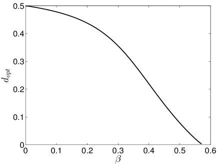
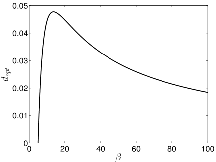
(a) (b)

Figure 1: K-optimal value  $d_{opt}$  for the three point design  $\boldsymbol{\xi}=\{0,d,1\}$  plotted against the parameter  $\beta$  for the intervals (a)  $]0,\beta^{*}[,\ \beta^{*}\approx 0.5718$,  and (b)  $]\beta^{**},100],\ \beta^{**}\approx 4.9586$.

2.1 Optimality of increasing domain equidistant designs

Consider an equidistant increasing domain design with step size  $d>0$,  that is the observation points are  $\boldsymbol{\xi}=\big{\{}0,d,2d,\ldots,(n-1)d\big{\}}$. In this case,  $p_{i}=\exp(-\beta d),\ i=1,2,\ldots,n-1,$  so the expressions in (2.4) reduce to

$$L_{1}(n) =\frac{2-n+n{\mathrm{e}}^{\beta d}}{{\mathrm{e}}^{\beta d}+1},\qquad\qquad L_{2}(n)=\frac{d(n-1)}{2}L_{1}(n),$$ (2.8)

$$L_{3}(n) =\frac{d^{2}(n-1)}{{\mathrm{e}}^{2\beta d}-1}\bigg{(}\frac{n(2n-1)({\mathrm{e}}^{\beta d}-1)^{2}}{6}+n\big{(}{\mathrm{e}}^{\beta d}-1\big{)}+1\bigg{)},$$

and the objective functions  $\mathcal{D}$,   $\mathcal{K}$  and  $\mathcal{R}$  defined by (2.5), (2.6) and (2.7), respectively, are univariate functions of  $d$.

Theorem 2.2

For model (2.1) with covariance structure (2.2) and equidistant increasing domain design with step size  $d>0$,  function  $\mathcal{D}$  is monotone increasing in  $d$,  whereas  $\mathcal{R}$  (and  $\mathcal{K}$)  has at least one global minimum point, that is, there exists a K-optimal design.

As a special case consider a two-point design  $\{0,d\}$.  Figures 2a and 2b show the behaviour of  ${\mathcal{D}}(d)$  and  ${\mathcal{K}}(d)$,  respectively, for  $\beta=0.1$,  whereas the following theorem formulates a general result on the two-point K-optimal design.

Theorem 2.3

For model (2.1) with covariance structure (2.2), there exists a unique K-optimal two-point design  $\{0,d_{opt}\}$,  where  $d_{opt}$  is the unique solution of

$$\big{(}d^{2}-2\big{)}{\mathrm{e}}^{3\beta d}+2(\beta d+1){\mathrm{e}}^{2\beta d}-\big{(}\beta d^{3}+d^{2}+2\beta d-2\big{)}{\mathrm{e}}^{\beta d}-2=0.$$ (2.9)

 

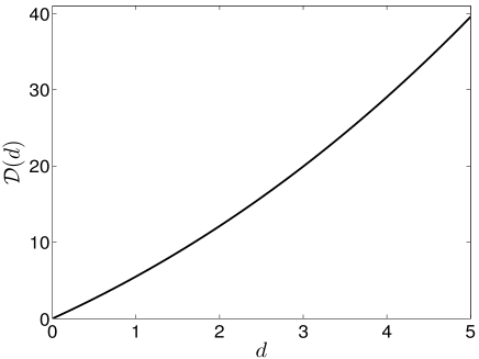
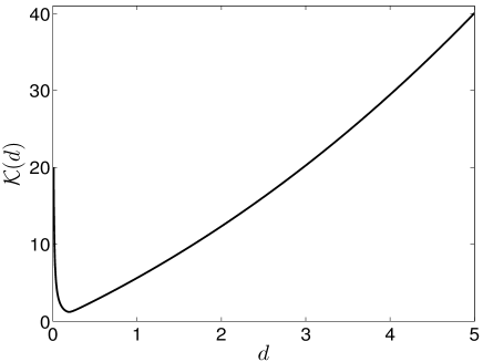
(a) (b)

Figure 2: Objective functions for two-point D-optimal (a) and K-optimal (b) designs with  $\beta=0.1$.

2.2 Comparison of equidistant designs

According to the ideas of Hoel, (1958), we investigate the change of D- and K-optimality criteria arising from doubling the number of sub-intervals in an equidistant partition of a fixed design interval, and we also study the situation when the length of the design interval is also doubled. The former approach refers to infill-, whereas the latter to increasing domain asymptotics.

Let the design space be  ${\mathcal{X}}=[a,b]\subset{\mathbb{R}},\ a<b$,  and denote by  $\widetilde{\mathcal{X}}$  the interval  $[2a,2b]$.  Obviously, without loss of generality we may assume  ${\mathcal{X}}=[0,1]$  and consider the sequences  $\boldsymbol{\xi}_{n}$  and  $\boldsymbol{\xi}_{2n}$  of designs on  ${\mathcal{X}}$,  where  $\boldsymbol{\xi}_{n}:=\big{\{}0,1/n,\ldots,(n-1)/n,1\big{\}},\ n\geq 2,\ n\in{\mathbb{N}}$,  and  designs  $\widetilde{\boldsymbol{\xi}}_{2n}:=\big{\{}0,1/n,\ldots,(2n-1)/n,2\big{\}}$  on  $\widetilde{\mathcal{X}}=[0,2]$.

Theorem 2.4

For model (2.1) with covariance structure (2.2)

$$\lim_{n\to\infty}\frac{{\mathcal{D}}(2n)}{{\mathcal{D}}(n)}=\lim_{n\to\infty}\frac{{\mathcal{K}}(2n)}{{\mathcal{K}}(n)}=1,$$ (2.10)

where  $\mathcal{D}(n)$  and  $\mathcal{K}(n)$  are the values of the objective functions (2.5) and (2.6), respectively, corresponding to the design  $\boldsymbol{\xi}_{n}$  on  ${\mathcal{X}}$.

Limits (2.10) show that for both investigated design criteria, if one has a dense enough equidistant partition of a fixed design space, there is no use of doubling the number of intervals in the partition, which is in accordance with the results of Hoel, (1958) for classical polynomial regression and Kiseľák and Stehlík, (2008) for OU processes with a constant trend.

Theorem 2.5

For model (2.1) with covariance structure (2.2)

$$\lim_{n\to\infty}\frac{\widetilde{\mathcal{D}}(2n)}{{\mathcal{D}}(n)}=D(\beta)\qquad\text{and}\qquad\lim_{n\to\infty}\frac{\widetilde{\mathcal{K}}(2n)}{{\mathcal{K}}(n)}=K(\beta),$$ (2.11)

with

$$D(\beta) :=\frac{16(\beta+1)(\beta^{2}+3\beta+3)}{(\beta+2)(\beta^{2}+6\beta+12)}\qquad\text{and}$$ (2.12)

$$K(\beta) :=\frac{(\beta+2)(\beta^{2}+6\beta+12)\big{(}7\beta^{2}+9\beta+3+\sqrt{37\beta^{4}+78\beta^{3}+51\beta^{2}+18\beta+9}\big{)}^{2}}{4(\beta+1)(\beta^{2}+3\beta+3)\big{(}4\beta^{2}+9\beta+3+\sqrt{13\beta^{4}+48\beta^{3}+33\beta^{2}-18\beta+9}\big{)}^{2}},$$

where  $\mathcal{D}(n)$  and  $\widetilde{\mathcal{D}}(2n)$  are the values of the objective function (2.5), whereas  $\mathcal{K}(n)$  and  $\widetilde{\mathcal{K}}(2n)$  are the values of the objective function (2.6) corresponding to the designs  $\boldsymbol{\xi}_{n}$  and  $\widetilde{\boldsymbol{\xi}}_{2n}$,  respectively.

Note that  $D(\beta)$  is strictly increasing with  $\lim_{\beta\to 0}D(\beta)=2$  and  $\lim_{\beta\to\infty}D(\beta)=16$,  whereas  $\lim_{\beta\to 0}K(\beta)=2$,  $K(\beta)$  has a single maximum of $2.3454$ at $0.2730$, and then it is strictly decreasing with  $\lim_{\beta\to\infty}K(\beta)=\big{(}7+\sqrt{37}\big{)}^{2}/\big{(}8+2\sqrt{13}\big{)}^{2}\approx 0.7397$.  Hence, doubling the interval over which the dense enough equidistant observations are made at least doubles the information on the unknown regression parameters  $(\alpha_{0},\alpha_{1})$,  which supports the extension of the design space. Moreover, after the maximum point of  $K(\beta)$  the larger the covariance parameter  $\beta$,  the more we gain in efficiency in terms of the condition number with extending the interval where the observations are made.

3 Ornstein-Uhlenbeck sheets with linear trend

As a spatial generalization of model (2.1), consider the spatial process

$$Y(s,t)=\alpha_{0}+\alpha_{1}s+\alpha_{2}t+U(s,t),$$ (3.1)

where the design points are taken from a compact design space  $\mathcal{X}=[a_{1},b_{1}]\times[a_{2},b_{2}]$,  with  $b_{1}>a_{1}$  and  $b_{2}>a_{2}$,  and  $U(s,t),\ s,t\in{\mathbb{R}}$,  is a stationary OU sheet, i.e., a centered Gaussian process with covariance structure

$${\mathsf{E}}\,U(s_{1},t_{1})U(s_{2},t_{2})=\frac{\sigma^{2}}{4\beta\gamma}\exp\big{(}-\beta|s_{1}-s_{2}|-\gamma|t_{1}-t_{2}|\big{)},$$ (3.2)

where  $\beta>0,\ \gamma>0,\ \sigma>0$.  Similar to the OU process,  $U(s,t)$  can be represented as

$$U(s,t)=\frac{\sigma}{2\sqrt{\beta\gamma}}{\mathrm{e}}^{-\beta s-\gamma t}{\mathcal{W}}\big{(}{\mathrm{e}}^{2\beta s},{\mathrm{e}}^{2\gamma t}\big{)},$$ (3.3)

where  ${\mathcal{W}}(s,t),\ s,t\in{\mathbb{R}}$,  is a standard Brownian sheet (Baran et al.,, 2003; Baran and Sikolya,, 2012). Again, we assume that the parameters  $\beta,\ \gamma$  and  $\sigma$  of the OU sheet  $U(s,t)$  driving model (3.1) are known.

We investigate regular grid designs of the form  $\big{\{}(s_{i},t_{j}):\ i=1,2,\ldots,n,\ j=1,2,\ldots,m\big{\}}\subset\mathcal{X}=[a_{1},b_{1}]\times[a_{2},b_{2}],\ n,m\geq 2$,  and without loss of generality we may assume  $a_{1}\leq s_{1}<s_{2}<\ldots<s_{n}\leq b_{1}$  and  $a_{2}\leq t_{1}<t_{2}<\ldots<t_{m}\leq b_{2}$  (Baran et al.,, 2015), and that  $U(s,t)$  has a unit variance. Again, the general form of the FIM  $\mathcal{I}_{\alpha_{0},\alpha_{1},\alpha_{2}}(n,m)$  on regression parameters  $\alpha_{0},\ \alpha_{1}$  and  $\alpha_{2}$  of model (3.1) based on observations  $\big{\{}Y(s_{i},t_{j}),\ i=1,2,\ldots,n,\ j=1,2,\ldots,m\big{\}}$  equals

$$\mathcal{I}_{\alpha_{0},\alpha_{1},\alpha_{2}}(n,m)=G(n,m)C(n,m)^{-1}G(n,m)^{\top},$$

where  $C(n,m)$  denotes the covariance matrix of the observations and

$$G(n,m):=\setcounter{MaxMatrixCols}{13}\begin{bmatrix}1&1&\cdots&1&1&1&\cdots&1&\cdots&1&1&\cdots&1\\ s_{1}&s_{1}&\cdots&s_{1}&s_{2}&s_{2}&\cdots&s_{2}&\cdots&s_{n}&s_{n}&\cdots&s_{n}\\ t_{1}&t_{2}&\cdots&t_{m}&t_{1}&t_{2}&\cdots&t_{m}&\cdots&t_{1}&t_{2}&\cdots&t_{m}\\ \end{bmatrix}.$$

The following theorem gives the exact form of the FIM  $I_{\alpha_{0},\alpha_{1},\alpha_{2}}(n,m)$.

Theorem 3.1

Consider the OU model (3.1) with covariance structure (3.2) observed in points  $\big{\{}(s_{i},t_{j}):\ i=1,2,\ldots,n,\ j=1,2,\ldots,m\big{\}}$.  Then

$$\mathcal{I}_{\alpha_{0},\alpha_{1},\alpha_{2}}(n,m)=\begin{bmatrix}L_{1}(n)M_{1}(m)&L_{2}(n)M_{1}(m)&L_{1}(n)M_{2}(m)\\ L_{2}(n)M_{1}(m)&L_{3}(n)M_{1}(m)&L_{2}(n)M_{2}(m)\\ L_{1}(n)M_{2}(m)&L_{2}(n)M_{2}(m)&L_{1}(n)M_{3}(m)\end{bmatrix}$$ (3.4)

with

$$L_{1}(n) :=\!1\!+\!\sum_{i=1}^{n-1}\frac{1\!-\!p_{i}}{1\!+\!p_{i}},\qquad\ L_{2}(n) :=\!s_{1}\!+\!\sum_{i=1}^{n-1}\frac{s_{i+1}\!-\!s_{i}p_{i}}{1\!+\!p_{i}},\qquad L_{3}(n) :=\!s_{1}^{2}\!+\!\sum_{i=1}^{n-1}\frac{(s_{i+1}\!-\!s_{i}p_{i})^{2}}{1\!-\!p_{i}^{2}},$$

$$M_{1}(m) :=\!1\!+\!\sum_{i=1}^{m-1}\frac{1\!-\!q_{i}}{1\!+\!q_{i}},\qquad M_{2}(m) :=\!t_{1}\!+\!\sum_{i=1}^{m-1}\frac{t_{i+1}\!-\!t_{i}q_{i}}{1\!+\!q_{i}},\qquad M_{3}(m) :=\!t_{1}^{2}\!+\!\sum_{i=1}^{m-1}\frac{(t_{i+1}\!-\!t_{i}q_{i})^{2}}{1\!-\!q_{i}^{2}},$$

where  $p_{i}:=\exp(-\beta d_{i})$  with   $d_{i}:=s_{i+1}-s_{i},\ \ i=1,2,\ldots,n-1$,  and  $q_{j}:=\exp(-\gamma\delta_{j})$  with $\delta_{j}:=t_{j+1}-t_{j},\ j=1,2,\ldots,m-1$.

Again, to simplify calculations we assume  $s_{1}=t_{1}=0$,  so the D-optimal design maximizes

$${\mathcal{D}}(\boldsymbol{d},\boldsymbol{\delta}):=\det\big{(}\mathcal{I}_{\alpha_{0},\alpha_{1},\alpha_{2}}(n,m)\big{)}=L_{1}(n)M_{1}(m)\big{(}L_{1}(n)L_{3}(n)-L_{2}^{2}(n)\big{)}\big{(}M_{1}(m)M_{3}(m)-M_{2}^{2}(m)\big{)}$$ (3.5)

both in  $\boldsymbol{d}=(d_{1},d_{2},\ldots,d_{n-1})$  and  $\boldsymbol{\delta}=(\delta_{1},\delta_{2},\ldots,\delta_{m-1})$,  whereas to obtain the K-optimal design one has to minimize the condition number  ${\mathcal{K}}(\boldsymbol{d},\boldsymbol{\delta})$  of  $\mathcal{I}_{\alpha_{0},\alpha_{1},\alpha_{2}}(n,m)$.  Using the expressions of Smith, (1961) for the eigenvalues of a $3\times 3$ symmetric matrix, one can easily show

$${\mathcal{K}}(\boldsymbol{d},\boldsymbol{\delta})=\frac{\mathrm{tr}\big{(}\mathcal{I}_{\alpha_{0},\alpha_{1},\alpha_{2}}(n,m)\big{)}+\sqrt{6\mathrm{tr}\big{(}\mathcal{I}_{\alpha_{0},\alpha_{1},\alpha_{2}}^{\,2}(n,m)\big{)}-2\mathrm{tr}^{2}\big{(}\mathcal{I}_{\alpha_{0},\alpha_{1},\alpha_{2}}(n,m)\big{)}}\cos(\varphi)}{\mathrm{tr}\big{(}\mathcal{I}_{\alpha_{0},\alpha_{1},\alpha_{2}}(n,m)\big{)}+\sqrt{6\mathrm{tr}\big{(}\mathcal{I}_{\alpha_{0},\alpha_{1},\alpha_{2}}^{\,2}(n,m)\big{)}-2\mathrm{tr}^{2}\big{(}\mathcal{I}_{\alpha_{0},\alpha_{1},\alpha_{2}}(n,m)\big{)}}\cos\big{(}\varphi+2\pi/3\big{)}},$$ (3.6)

where  $\varphi:=\frac{1}{3}\arccos(\varrho)\in[0,\pi/3]$,  with

$$\varrho:=\frac{54\det\big{(}\mathcal{I}_{\alpha_{0},\alpha_{1},\alpha_{2}}(n,m)\big{)}+\mathrm{tr}\big{(}\mathcal{I}_{\alpha_{0},\alpha_{1},\alpha_{2}}(n,m)\big{)}\Big{(}9\mathrm{tr}\big{(}\mathcal{I}_{\alpha_{0},\alpha_{1},\alpha_{2}}^{\,2}(n,m)\big{)}-5\mathrm{tr}^{2}\big{(}\mathcal{I}_{\alpha_{0},\alpha_{1},\alpha_{2}}(n,m)\big{)}\Big{)}}{\sqrt{2}\Big{(}3\mathrm{tr}\big{(}\mathcal{I}_{\alpha_{0},\alpha_{1},\alpha_{2}}^{\,2}(n,m)\big{)}-\mathrm{tr}^{2}\big{(}\mathcal{I}_{\alpha_{0},\alpha_{1},\alpha_{2}}(n,m)\big{)}\Big{)}^{3/2}}.$$

Example 3.2

Let the design space be the unit square  $\mathcal{X}=[0,1]^{2}$  and consider a nine-point restricted regular grid design, where  $s_{1}=t_{1}=0,\ s_{2}=d,\ t_{2}=\delta,\ s_{3}=t_{3}=1$,  with  $0\leq d,\delta\leq 1$.  In this case the FIM (3.1) equals

$$\mathcal{I}_{\alpha_{0},\alpha_{1},\alpha_{2}}(d,\delta)=\begin{bmatrix}L_{1}(d)M_{1}(\delta)&L_{2}(d)M_{1}(\delta)&L_{1}(d)M_{2}(\delta)\\ L_{2}(d)M_{1}(\delta)&L_{3}(d)M_{1}(\delta)&L_{2}(d)M_{2}(\delta)\\ L_{1}(d)M_{2}(\delta)&L_{2}(d)M_{2}(\delta)&L_{1}(d)M_{3}(\delta)\end{bmatrix}$$

with

$$L_{1}(d) \!:=\!\frac{2}{1\!+\!{\mathrm{e}}^{-\beta d}}\!+\!\frac{1\!-\!{\mathrm{e}}^{-\beta(1-d)}}{1\!+\!{\mathrm{e}}^{-\beta(1-d)}},\ L_{2}(d) \!:=\!\frac{d}{1\!+\!{\mathrm{e}}^{-\beta d}}\!+\!\frac{1\!-\!d{\mathrm{e}}^{-\beta(1-d)}}{1\!+\!{\mathrm{e}}^{-\beta(1-d)}},\ L_{3}(d) \!:=\!\frac{d^{2}}{1\!-\!{\mathrm{e}}^{-2\beta d}}\!+\!\frac{(1\!-\!d{\mathrm{e}}^{-\beta(1-d)})^{2}}{1\!-\!{\mathrm{e}}^{-2\beta(1-d)}},$$

$$M_{1}(\delta) \!:=\!\frac{2}{1\!+\!{\mathrm{e}}^{-\gamma\delta}}\!+\!\frac{1\!-\!{\mathrm{e}}^{-\gamma(1-\delta)}}{1\!+\!{\mathrm{e}}^{-\gamma(1-\delta)}},\ M_{2}(\delta) \!:=\!\frac{\delta}{1\!+\!{\mathrm{e}}^{-\gamma\delta}}\!+\!\frac{1\!-\!\delta{\mathrm{e}}^{-\gamma(1-\delta)}}{1\!+\!{\mathrm{e}}^{-\gamma(1-\delta)}},\ M_{3}(\delta) \!:=\!\frac{\delta^{2}}{1\!-\!{\mathrm{e}}^{-2\gamma\delta}}\!+\!\frac{(1\!-\!\delta{\mathrm{e}}^{-\gamma(1-\delta)})^{2}}{1\!-\!{\mathrm{e}}^{-2\gamma(1-\delta)}},$$

so both the determinant  $\mathcal{D}$  and the condition number  $\mathcal{K}$  of  $\mathcal{I}_{\alpha_{0},\alpha_{1},\alpha_{2}}(d,\delta)$   are bivariate functions of  $d$  and  $\delta$.  As for all possible parameter values  $\beta>0$  function  $L_{1}(d)$  reaches its unique maximum at  $d=1/2$,  and obviously the same holds for  $M_{1}(\delta)$  for all  $\gamma>0$,  representations (2.5) and (3.5) together with the results of Example 2.1 imply that the D-optimal nine-point restricted regular grid design is directionally equidistant.

Similar to the temporal case of Example 2.1, a non-collapsing K-optimal design exists only outside a certain region of the  $(\beta,\gamma)$  parameter space. In Figures 3a and 3b the  $d_{opt}$  and  $\delta_{opt}$  coordinates of the minimum point of  $\mathcal{K}(d,\delta)$ are plotted as functions of parameters, where $0$ values correspond to collapsing designs, whereas Figures 3c and 3d display the corresponding contour plots.

 

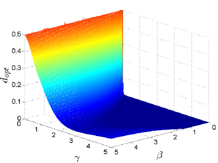
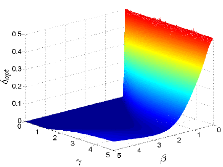
(a) (b)

 

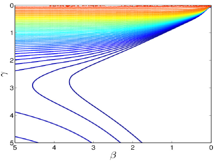
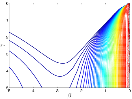
(c) (d)

Figure 3: $d_{opt}$ (a) and  $\delta_{opt}$ (b) coordinates of the minimum point of the objective function  $\mathcal{K}(d,\delta)$  and the corresponding contour plots  ($d_{opt}$: (c);  $\delta_{opt}$: (d)) for a nine-point restricted regular grid design.

3.1 Optimality of increasing domain equidistant designs

Consider now the directionally equidistant regular grid design with step sizes  $d>0$  and  $\delta>0$  consisting of observation locations  $\boldsymbol{\xi}=\big{\{}\big{(}(i\!-\!1)d,(j\!-\!1)\delta\big{)}:\ i=1,2,\ldots,n,\ j=1,2,\ldots,m\big{\}}$.  In this situation,  $L_{1}(n),\ L_{2}(n)$  and  $L_{3}(n)$ have forms given by (2.8), and in a similar way we have

$$M_{1}(m) =\frac{2-m+m{\mathrm{e}}^{\gamma\delta}}{{\mathrm{e}}^{\gamma\delta}+1},\qquad\qquad M_{2}(m)=\frac{\delta(m-1)}{2}M_{1}(m),$$ (3.7)

$$M_{3}(m) =\frac{\delta^{2}(m-1)}{{\mathrm{e}}^{2\gamma\delta}-1}\bigg{(}\frac{m(2m-1)({\mathrm{e}}^{\gamma\delta}-1)^{2}}{6}+m\big{(}{\mathrm{e}}^{\gamma\delta}-1\big{)}+1\bigg{)}.$$

Hence, objective functions  $\mathcal{D}$  and  $\mathcal{K}$  are bivariate functions of  $d$  and  $\delta$.

Theorem 3.3

For model (3.1) with covariance structure (3.2) and directionally equidistant increasing domain design with step sizes  $d>0$  and  $\delta>0$,  function  $\mathcal{D}$  is monotone increasing both in  $d$  and  $\delta$.

Similar to Section 2.1, in case of K-optimality one faces a different situation.

Example 3.4

Consider the four-point increasing domain regular grid design  $\big{\{}(0,0),(d,0),(0,\delta),(d,\delta)\big{\}}$  for the process (3.1) with parameters  $\beta=0.2,\ \gamma=0.3$.  By Theorem 3.3, there is no D-optimal design, whereas Figures 4a and 4b showing the objective function  $\mathcal{K}(d,\delta)$  and the corresponding contour plot, respectively, clearly indicate the existence of a K-optimal design.

 

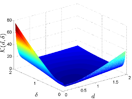
(a) (b)

Figure 4: Objective function  $\mathcal{K}(d,\delta)$  (a) and the corresponding contour plot (b) of a four-point regular grid design with  $\beta=0.2,\ \gamma=0.3$.

3.2 Comparison of equidistant designs

Again, given a fixed design space  ${\mathcal{X}}=[a_{1},b_{1}]\times[a_{2},b_{2}],\ a_{1}<b_{1},\ a_{2}<b_{2}$,  we are interested in the effect of refining the directionally equidistant regular grid design by doubling the number of partition intervals in one direction (by symmetry it suffices to deal, for instance, with the first coordinate) or in both coordinate directions. Further, we also consider the case when doubling of the partition intervals in a given coordinate direction is combined with doubling the corresponding dimension of the design space. Obviously, assumption  ${\mathcal{X}}=[0,1]^{2}$  does not violate generality, and we may consider designs  $\boldsymbol{\xi}_{n,m}$,  $\boldsymbol{\xi}_{2n,m}$  and  $\boldsymbol{\xi}_{2n,2m}$,  on  $\mathcal{X}$  with  $\boldsymbol{\xi}_{n,m}:=\big{\{}(i/n,j/m):i=0,1,\ldots,n,\ j=0,1,\ldots,m\big{\}},\ n,m\!\geq\!2,\ n,m\in{\mathbb{N}}$,  design  $\widetilde{\boldsymbol{\xi}}_{2n,2m}:=\big{\{}(i/n,j/m):i=0,1,\ldots,2n,\ j=0,1,\ldots,2m\big{\}}$  on  $\widetilde{\mathcal{X}}:=[0,2]^{2}$  and  $\widehat{\boldsymbol{\xi}}_{2n,m}:=\big{\{}(i/n,j/m):i=0,1,\ldots,2n,\ j=0,1,\ldots,m\big{\}}$  on  $\widehat{\mathcal{X}}:=[0,2]\times[0,1]$.

Theorem 3.5

For model (3.1) with covariance structure (3.2)

$$\lim_{n,m\to\infty}\frac{{\mathcal{D}}(2n,2m)}{{\mathcal{D}}(n,m)}=\lim_{n,m\to\infty}\frac{{\mathcal{D}}(2n,m)}{{\mathcal{D}}(n,m)}=\lim_{n,m\to\infty}\frac{{\mathcal{K}}(2n,2m)}{{\mathcal{K}}(n,m)}=\lim_{n,m\to\infty}\frac{{\mathcal{K}}(2n,m)}{{\mathcal{K}}(n,m)}=1,$$

where  $\mathcal{D}(n,m)$  and  $\mathcal{K}(n,m)$  are the values of the objective functions (3.5) and (3.6), respectively, corresponding to the design  $\boldsymbol{\xi}_{n,m}$  on  ${\mathcal{X}}$.

Using Theorem 3.5, on can formulate a similar conclusion as in the case of OU processes. In particular, after a sufficiently large amount of grid design points there is no need of further refinement of the grid.

Theorem 3.6

For model (3.1) with covariance structure (3.2)

$$\lim_{n,m\to\infty}\frac{\widetilde{\mathcal{D}}(2n,2m)}{{\mathcal{D}}(n,m)}\!=\!\widetilde{D}(\beta)\widetilde{D}(\gamma)\quad\text{and}\quad\lim_{n,m\to\infty}\frac{\widehat{\mathcal{D}}(2n,m)}{{\mathcal{D}}(n,m)}\!=\!\widetilde{D}(\beta),\qquad\text{with}\qquad\widetilde{D}(\beta)\!:=\!\frac{2(\beta\!+\!1)}{\beta\!+\!2}D(\beta),$$

where  $D(\beta)$  is defined by (2.12), whereas  $\widetilde{\mathcal{D}}(2n,2m)$  and  $\widehat{\mathcal{D}}(2n,m)$  denote the values of the objective function (3.5) corresponding to designs   $\widetilde{\boldsymbol{\xi}}_{2n,2m}$  and  $\widehat{\boldsymbol{\xi}}_{2n,m}$,  respectively.

 

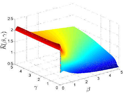
(a) (b)

Figure 5: Limiting functions  $\widetilde{K}(\beta,\gamma)$  (a) and  $\widehat{K}(\beta,\gamma)$  (b) of  $\widetilde{\mathcal{K}}(2n,2m)/{\mathcal{K}}(n,m)$  and  $\widehat{\mathcal{K}}(2n,m)/{\mathcal{K}}(n,m)$  as  $n,m\to\infty$.

As  $\widetilde{D}(\beta)$  is strictly increasing with  $\lim_{\beta\to 0}\widetilde{D}(\beta)=2$  and  $\lim_{\beta\to\infty}\widetilde{D}(\beta)=32$,  if one has a dense enough directionally equidistant grid of observations, the extension of the design space along a coordinate direction will at least double the information on the unknown regression parameters $(\alpha_{0},\alpha_{1},\alpha_{2})$.

Now, denote by $\widetilde{\mathcal{K}}(2n,2m)$  and  $\widehat{\mathcal{K}}(2n,m)$   the values of the objective function (3.6) corresponding to designs   $\widetilde{\boldsymbol{\xi}}_{2n,2m}$  and  $\widehat{\boldsymbol{\xi}}_{2n,m}$,  respectively, and let

$$\widetilde{K}(\beta,\gamma):=\lim_{n,m\to\infty}\frac{\widetilde{\mathcal{K}}(2n,2m)}{{\mathcal{K}}(n,m)}\qquad\text{and}\qquad\widehat{K}(\beta,\gamma):=\lim_{n,m\to\infty}\frac{\widehat{\mathcal{K}}(2n,m)}{{\mathcal{K}}(n,m)}.$$

Due to the very complicated form of the objective function (3.6) one cannot provide feasible expressions for the limiting functions $\widetilde{K}(\beta,\gamma)$  and  $\widehat{K}(\beta,\gamma)$,  plotted in Figures 5a and 5b, respectively. In contrast to the D-optimal design,  $\widehat{K}(\beta,\gamma)$  depends not only on  $\beta$.  Moreover, there is a substantial difference compared to the one dimensional case, since  $\widetilde{K}(\beta,\gamma)$  seems to have a maximum point.

4 Simulation results

 

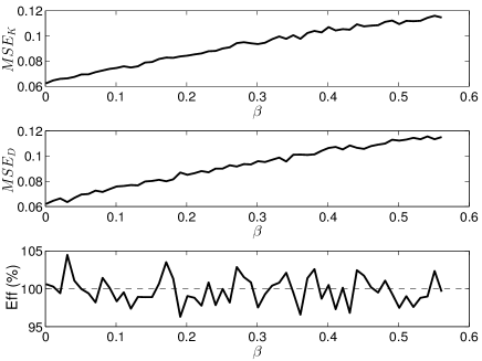
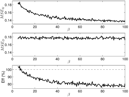
(a) (b)

Figure 6: Average mean squared errors  $\mathrm{MSE}_{K}$  and  $\mathrm{MSE}_{D}$  of GLS estimates of parameters based on three-point restricted K- and D-optimal designs and relative efficiency  ($\mathrm{Eff}:={\mathrm{MSE}_{K}}/{\mathrm{MSE}_{D}}\times 100\%$)  plotted against the parameter  $\beta$  for the intervals (a)  $]0,\beta^{*}[,\ \beta^{*}\approx 0.5718$,  and (b)   $]\beta^{**},100],\ \beta^{**}\approx 4.9586$,  respectively.

To illustrate the differences between K- and D-optimal designs, computer simulations using Matlab R2014a are performed. In general, the driving stationary Ornstein-Uhlenbeck processes and fields of models (2.1) and (3.1), respectively, can be simulated either with the help of discretization (see, e.g., Gillespie,, 1996) or using their Karhunen-Loève expansions based on representations (2.3) and (3.3) (Jaimez and Bonnet,, 1987; Baran and Sikolya,, 2012). However, in our simulation study, due to the small number of locations, it is sufficient to draw samples from the corresponding finite dimensional distributions.

In each of the following examples,  $10000$  independent samples of the driving Gaussian processes are simulated and the average mean squared errors (MSE) of the generalized least squares (GLS) estimates of the regression parameters based on samples corresponding to different designs are calculated.

Example 4.1

Consider the model (2.1) with true parameter values  $\alpha_{0}=\alpha_{1}=1$  and standard deviation parameter  $\sigma=1/4$  defined on the unit interval  $[0,1]$,  and the three-point restricted design  $\{0,d,1\}$.  As it has been mentioned in Example 2.1, the D-optimal design for all  $\beta>0$  is equidistant, whereas K-optimal design exists only for parameter values  $0<\beta<\beta^{*}\approx 0.5718$  and  $\beta>\beta^{**}\approx 4.9586$.

Figures 6a and 6b display the average mean squared errors  $\mathrm{MSE}_{K}$  and  $\mathrm{MSE}_{D}$  of the GLS estimates of parameters based on K- and D-optimal designs plotted against the parameter  $\beta$  together with the relative efficiency

$$\mathrm{Eff}:=\frac{\mathrm{MSE}_{K}}{\mathrm{MSE}_{D}}\times 100\%$$ (4.1)

for the intervals  $]0,\beta^{*}[$  and  $]\beta^{**},100]$,  respectively. Observe that for small parameter values the difference in MSE is negligible, whereas for parameters from the upper interval the K-optimal design exhibits a superior overall performance.

Example 4.2

Consider the model (3.1) with true parameter values  $\alpha_{0}=\alpha_{1}=\alpha_{1}=1$  and standard deviation parameter  $\sigma=1/4$  defined on the unit square  $[0,1]^{2}$,  and the nine-point restricted regular grid design  $\{(0,0),(0,\delta),(0,1),(d,0),(d,\delta),(d,1),(1,0),(1,\delta),(1,1)\}$.  According to the results of Example 3.2, for all positive values of  $\beta$  and  $\gamma$  the D-optimal design is directionally equidistant, that is  $d=\delta=1/2$,  whereas a non-collapsing K-optimal design exists only in a certain region of the parameter space, see Figure 3.

$\beta\setminus\gamma$ 0.01 0.03 0.05 0.10 0.15 0.01 100.88 99.45 97.53 101.60 96.92 0.03 99.43 101.54 100.12 99.22 104.38 0.05 100.79 100.33 102.00 97.51 97.46 0.10 101.37 99.91 99.61 99.86 99.66 0.15 100.94 99.51 102.65 98.48 102.48    $\beta\setminus\gamma$ 10 15 20 25 30 10 115.33 109.19 105.53 102.89 99.14 15 108.18 104.65 96.49 95.25 93.80 20 103.93 100.66 95.09 93.61 93.70 25 100.50 95.92 94.18 93.20 89.28 30 102.91 96.98 94.14 90.04 88.90

Table 1: Relative efficiency $\mathrm{Eff}$ (%) of MSEs of GLS estimates of regression parameters based on nine-point restricted K- and D-optimal regular grid designs for various values of  $\beta$  and  $\gamma$.

In Table 1 the relative efficiencies (4.1) of the MSEs of the GLS estimates of regression parameters based on nine-point restricted K- and D-optimal regular grid designs are reported for different values of  $\beta$  and  $\gamma$.  Similar to the temporal case of Example 4.1, for large parameter values, if a non-collapsing K-optimal design exists, it will outperform the corresponding D-optimal one.

5 Conclusions

We investigate the properties of K-optimal designs for temporal and spatial linear regression models driven by OU processes and sheets, respectively, and highlight the differences compared with the corresponding D-optimal sampling. We study the problems of existence of K-optimal designs and also investigate the dependence of the two designs on the covariance parameters of the driving processes. This information may be crucial for an experimenter in order to increase efficiency in practical situations. Simulation results display the superiority of restricted K-optimal designs for large covariance parameter values.

Acknowledgments

This research was supported by the János Bolyai Research Scholarship of the Hungarian Academy of Sciences and by the Hungarian – Austrian intergovernmental S&T cooperation program TÉT_15-1-2016-0046. The author is indebted to Milan Stehlík for his valuable suggestions and remarks.

Appendix A Appendix

A.1 Correlation structure of observations

The correlation matrix of observations  $\big{\{}Y(s_{i}),\ i=1,2,\ldots,n\big{\}},\ n\geq 2,$  of the stochastic process (2.1) equals

$$C(n)=\begin{bmatrix}1&p_{1}&p_{1}p_{2}&p_{1}p_{2}p_{3}&\dots&\dots&\prod_{i=1}^{n-1}p_{i}\\ p_{1}&1&p_{2}&p_{2}p_{3}&\dots&\dots&\prod_{n=2}^{n-1}p_{i}\\ p_{1}p_{2}&p_{2}&1&p_{3}&\dots&\dots&\prod_{i=3}^{n-1}p_{i}\\ p_{1}p_{2}p_{3}&p_{2}p_{3}&p_{3}&1&\dots&\dots&\vdots\\ \vdots&\vdots&\vdots&\vdots&\ddots&&\vdots\\ \vdots&\vdots&\vdots&\vdots&&\ddots&p_{n-1}\\ \prod_{i=1}^{n-1}p_{i}&\prod_{i=2}^{n-1}p_{i}&\prod_{i=3}^{n-1}p_{i}&\dots&\dots&p_{n-1}&1\\ \end{bmatrix},$$

where  $p_{i}:=\exp(-\beta d_{i})$   and  $d_{i}:=s_{i+1}-s_{i},\ i=1,2,\ldots,n-1$.  According to the results of Kiseľák and Stehlík, (2008), the inverse of  $C(n)$  is given by

$$C^{-1}(n)=\begin{bmatrix}\frac{1}{1-p_{1}^{2}}&\frac{p_{1}}{p_{1}^{2}-1}&0&0&\dots&\dots&0\\ \frac{p_{1}}{p_{1}^{2}-1}&V_{2}&\frac{p_{2}}{p_{2}^{2}-1}&0&\dots&\dots&0\\ 0&\frac{p_{2}}{p_{2}^{2}-1}&V_{3}&\frac{p_{3}}{p_{3}^{2}-1}&\dots&\dots&0\\ 0&0&\frac{p_{3}}{p_{3}^{2}-1}&V_{4}&\dots&\dots&\vdots\\ \vdots&\vdots&\vdots&\vdots&\ddots&&\vdots\\ \vdots&\vdots&\vdots&\vdots&&V_{n-1}&\frac{p_{n-1}}{p_{n-1}^{2}-1}\\ 0&0&0&\dots&\dots&\frac{p_{n-1}}{p_{n-1}^{2}-1}&\frac{1}{1-p_{n-1}^{2}}\\ \end{bmatrix},$$

where  $V_{k}:=\frac{1-p_{k}^{2}p_{k-1}^{2}}{(p_{k}^{2}-1)(p_{k-1}^{2}-1)}=\frac{1}{1-p_{k}^{2}}+\frac{p_{k-1}^{2}}{1-p_{k-1}^{2}},\ k=2,\dots,n-1$.

A.2 Proof of Theorem 2.2

Using form (2.8) of the entries of the information matrix, a short calculation shows

$${\mathcal{D}}(d)=J_{n}(\beta d)\frac{n\!-\!1}{\beta^{2}}F_{n}(\beta d),$$

with

$$J_{n}(d):=\frac{2\!-\!n\!+\!n{\mathrm{e}}^{d}}{{\mathrm{e}}^{d}\!+\!1}\geq 1\quad\text{and}\quad F_{n}(d):=\frac{d^{2}}{{\mathrm{e}}^{2d}\!-\!1}\left(\frac{n(n\!+\!1)}{12}\big{(}{\mathrm{e}}^{d}\!-\!1\big{)}^{2}\!+\!\frac{n\!+\!1}{2}\big{(}{\mathrm{e}}^{d}\!-\!1\big{)}\!+\!1\right)\geq 0,$$ (A.1)

where  $J_{n}(d)$  is a strictly increasing function of  $d$.  Hence, in order to prove the first statement of Theorem 2.2, it suffices to show that  $F_{n}(d)$  is also strictly increasing for all integers  $n\geq 2$.  This latter property obviously holds for

$$F_{2}(d)=\frac{d^{2}}{2(1-{\mathrm{e}}^{-d})}\qquad\text{and}\qquad F_{3}(d)=\frac{d^{2}}{1-{\mathrm{e}}^{-2d}},$$

whereas for  $n\geq 4$  one can consider the decomposition

$$F_{n}(d)=F_{3}(d)G_{n}(d),\qquad\text{where}\qquad G_{n}(d):=\frac{1}{{\mathrm{e}}^{2d}}\left(\frac{n(n+1)}{12}\big{(}{\mathrm{e}}^{d}-1\big{)}^{2}+\frac{n+1}{2}\big{(}{\mathrm{e}}^{d}-1\big{)}+1\right).$$

A short calculation shows that the numerator of  $G^{\prime}_{n}(d)$  equals

$$\frac{{\mathrm{e}}^{2d}(n-3)}{6}\big{(}{\mathrm{e}}^{d}(n+1)-n+2\big{)}\geq\frac{{\mathrm{e}}^{2d}(n-3)}{2}>0,$$

which completes the proof of monotonicity of  ${\mathcal{D}}(d)$.

Now, (2.7) and (2.8) imply

$$\mathcal{R}(d)=\frac{\Big{(}n({\mathrm{e}}^{\beta d}\!-\!1)^{2}\big{(}(n\!-\!1)(2n\!-\!1)d^{2}+6\big{)}/6+({\mathrm{e}}^{\beta d}\!-\!1)\big{(}n(n\!-\!1)d^{2}+2\big{)}+(n\!-\!1)d^{2}\Big{)}^{2}}{d^{2}(n\!-\!1)({\mathrm{e}}^{\beta d}\!-\!1)\big{(}n(n\!+\!1)({\mathrm{e}}^{\beta d}\!-\!1)^{2}/12+(n\!+\!1)({\mathrm{e}}^{\beta d}\!-\!1)/2+1\big{)}\big{(}n({\mathrm{e}}^{\beta d}\!-\!1)+2\big{)}}.$$ (A.2)

After dividing both the numerator and the denominator of the right-hand side of (A.2) by  ${\mathrm{e}}^{4\beta d}$,  one can easily see

$$\lim_{d\to\infty}\mathcal{R}(d)=\lim_{d\to\infty}\frac{n^{2}\big{(}(n-1)(2n-1)d^{2}+6\big{)}^{2}}{3n^{2}\big{(}n^{2}-1\big{)}d^{2}}=\infty.$$ (A.3)

In a similar way, taking into account that  $\lim_{d\to 0}\big{(}{\mathrm{e}}^{d}-1\big{)}/d=1$,  the division of both the numerator and the denominator of  ${\mathcal{R}}(d)$  by  $d^{2}({\mathrm{e}}^{\beta d}-1)$  results in

$$\lim_{d\to 0}\mathcal{R}(d)=\lim_{d\to 0}\frac{\Big{(}nd^{1/2}\big{(}(n-1)(2n-1)d^{2}+6\big{)}/6+\big{(}n(n-1)d^{3/2}+2d^{-1/2}\big{)}+(n-1)d^{1/2}\Big{)}^{2}}{2(n-1)}=\infty,$$

which together with (A.3) implies that  $\mathcal{R}(d)$  should have at least one global minimum. $\square$

A.3 Proof of Theorem 2.3

For  $n=2$  expression (A.2) simplifies to

$$\mathcal{R}(d)=\frac{\big{(}(d^{2}+2){\mathrm{e}}^{\beta d}-2\big{)}^{2}}{d^{2}\big{(}{\mathrm{e}}^{2\beta d}-1\big{)}},$$

and

$$\mathcal{R}^{\prime}(d)=\frac{2\big{(}(d^{2}\!+\!2){\mathrm{e}}^{\beta d}\!-\!2\big{)}}{d^{3}\big{(}{\mathrm{e}}^{2\beta d}\!-\!1\big{)}^{2}}R(d)\quad\text{with}\quad R(d):=(d^{2}-2){\mathrm{e}}^{3\beta d}+2(\beta d+1){\mathrm{e}}^{2\beta d}-(\beta d^{3}+d^{2}+2\beta d-2){\mathrm{e}}^{\beta d}-2.$$

For  $d\geq 0$  the derivative  $\mathcal{R}^{\prime}(d)$  equals  $0$  if and only if equation (2.9) holds, that is  $R(d)=0$.  Hence, to complete the proof of Theorem 2.3, it remains two show that (2.9) has a unique non-negative solution and this solution is the minimum of  $\mathcal{R}(d)$.  Now, observe that  $R(d)$  admits the representation

$$R(d)=d^{2}R^{(1)}(\beta d)-2R^{(2)}(\beta d),$$

where

$$R^{(1)}(x):={\mathrm{e}}^{x}\big{(}{\mathrm{e}}^{2x}-x-1\big{)}>0\quad\text{and}\quad R^{(2)}(x):=\Big{(}{\mathrm{e}}^{x}\big{(}{\mathrm{e}}^{x}-x-1\big{)}+\big{(}{\mathrm{e}}^{x}-1\big{)}\Big{)}\big{(}{\mathrm{e}}^{x}-1\big{)}>0,\ \ \text{for}\ \ x>0.$$

In this way

$$R(d)=0\qquad\text{if and only if}\qquad\frac{d^{2}}{2}=\frac{R^{(2)}(\beta d)}{R^{(1)}(\beta d)}.$$ (A.4)

A short calculation shows that  ${R^{(2)}(x)}/{R^{(1)}(x)}$  is strictly monotone increasing and strictly concave. Further, we have

$$\lim_{x\to 0}\frac{R^{(2)}(x)}{R^{(1)}(x)}=0\qquad\text{and}\qquad\lim_{x\to\infty}\frac{R^{(2)}(x)}{R^{(1)}(x)}=1.$$

Hence, by the convexity of  $d^{2}/2$,  for all  $\beta>0$  the equation on the right hand side of (A.4) has a single solution (obviously, depending on  $\beta$).  Moreover, as for all  $\beta>0$,

$$\lim_{d\to 0}R(d)=0\qquad\text{and}\qquad\lim_{d\to\infty}R(d)=\infty,$$

if  $R(d)$  has a change of sign at this unique root, the change shall be from negative to positive. This means that the solution of (2.9) is the unique minimum of  $\mathcal{R}(d)$.  Thus, it remains to show that for all  $\beta>0$,  one can find some  $d>0$  such that  $R(d)<0$.

Consider the decomposition

$$R(d)={\mathrm{e}}^{\beta d}\big{(}d^{2}Q^{(1)}(d)-2{\mathrm{e}}^{\beta d}Q^{(2)}(d)\big{)}-2Q^{(3)}(d),$$

where

$$Q^{(1)}(d):={\mathrm{e}}^{2\beta d}-\beta^{2}\Big{(}\frac{\beta d}{3}+1\Big{)}{\mathrm{e}}^{\beta d}-\beta d-1,$$

$$Q^{(2)}(d):={\mathrm{e}}^{\beta d} \,-\Big{(}\frac{\beta^{3}d^{3}}{6}+\frac{\beta^{2}d^{2}}{2}+\beta d+1\Big{)},\qquad Q^{(3)}(d):={\mathrm{e}}^{\beta d}(\beta d-1)+1.$$

Using Taylor series expansions one can easily see that for all  $x>0$

$$1-x<{\mathrm{e}}^{-x}\qquad\text{and}\qquad 1+x+\frac{x^{2}}{2}+\frac{x^{3}}{6}<{\mathrm{e}}^{x},$$

implying for all  $d>0$  and  $\beta>0$  the positivity of  $Q^{(3)}(d)$  and  $Q^{(2)}(d)$,  respectively. Finally,

$$\lim_{d\to 0}Q^{(1)}(d)=-\beta^{2}\qquad\text{and}\qquad\lim_{d\to\infty}Q^{(1)}(d)=\infty,$$

thus, for all  $\beta>0$  there exist a  $d>0$  such that  $Q^{(1)}(d)<0$,  which completes the proof. $\square$

A.4 Proof of Theorem 2.4

Under the settings of the theorem  ${\mathcal{D}}(n)=L_{1}(n+1)L_{3}(n+1)-L_{2}^{2}(n+1)$  and  ${\mathcal{K}}(n)=g\big{(}\mathcal{R}(n)\big{)}$  with  ${\mathcal{R}}(n)=\big{(}L_{1}(n+1)+L_{3}(n+1)\big{)}^{2}/\mathcal{D}(n)$  and  $g(x):=\frac{1}{4}\big{(}\sqrt{x}+\sqrt{x-4}\big{)}^{2}$,  where the expressions for  $L_{1}(n+1),\ L_{2}(n+1)$  and  $L_{3}(n+1)$  can be obtained using (2.8) with  $d=1/n$.  Since for all  $\beta>0$

$$\lim_{n\to\infty}n\big{(}{\mathrm{e}}^{\beta/n}-1\big{)}=\beta,$$

one can easily show

$$\lim_{n\to\infty}L_{1}(n+1)= \lim_{n\to\infty}L_{1}(2n+1)=\frac{\beta}{2}+1,\qquad\lim_{n\to\infty}L_{2}(n+1)=\lim_{n\to\infty}L_{2}(2n+1)=\frac{\beta}{4}+\frac{1}{2},$$ (A.5)

$$\lim_{n\to\infty}L_{3}(n+1)=\lim_{n\to\infty}L_{3}(2n+1)=\frac{1}{2\beta}\left(\frac{\beta^{2}}{3}+\beta+1\right),$$

which completes the proof. $\square$

A.5 Proof of Theorem 2.5

Similar to the proof of Theorem 2.4 we have  $\widetilde{\mathcal{D}}(2n)=\widetilde{L}_{1}(2n+1)\widetilde{L}_{3}(2n+1)-\widetilde{L}_{2}^{2}(2n+1)$  and  $\widetilde{\mathcal{K}}(2n)=g\big{(}\widetilde{\mathcal{R}}(2n)\big{)}$  with  $\widetilde{\mathcal{R}}(2n)=\big{(}\widetilde{L}_{1}(2n+1)+\widetilde{L}_{3}(2n+1)\big{)}^{2}/\widetilde{\mathcal{D}}(2n)$,  where now the expressions for  $\widetilde{L}_{1}(2n+1),\ \widetilde{L}_{2}(2n+1)$  and  $\widetilde{L}_{3}(2n+1)$  can be obtained using (2.8) for  $2n+1$  design points with  $d=1/n$.  Hence, the limits in (2.11) are direct consequences of (A.5) and

$$\lim_{n\to\infty}\widetilde{L}_{1}(2n+1)=\beta+1,\qquad\lim_{n\to\infty}\widetilde{L}_{2}(2n+1)=\beta+1,\qquad\lim_{n\to\infty}\widetilde{L}_{3}(2n+1)=\frac{1}{\beta}\left(\frac{4}{3}{\beta^{2}}+2\beta+1\right).$$

$\square$

A.6 Proof of Theorem 3.1

For the regular grid design introduced in Section 3, the covariance matrix  $C(n,m)$  of observations admits the decomposition

$$C(n,m)=P(n)\otimes Q(m),$$

where  $P(n)$  and  $Q(m)$  are covariance matrices of observations of OU processes with covariance parameters  $\beta>0$  and  $\gamma>0$  in time points  $s_{1}<s_{2}<\ldots<s_{n}$  and  $t_{1}<t_{2}<\ldots<t_{m}$, respectively (see Baran et al., (2014) or the online supplement of Baran et al., (2015)). In this way,

$$C^{-1}(n,m)=P^{-1}(n)\otimes Q^{-1}(m),$$ (A.6)

where for the exact forms of $P^{-1}(n)$  and  $Q^{-1}(m)$  see A.1. Further,

$$G(n,m)=S(n)\otimes{\mathbf{1}}_{m}^{\top}+{\mathbf{1}}_{n}^{\top}\otimes T(m),$$ (A.7)

where  ${\mathbf{1}}_{n},\ n\in{\mathbb{N}},$  denotes the column vector of ones of length  $n$,

$$S(n):=\begin{bmatrix}1/2&1/2&\cdots&1/2\\ s_{1}&s_{2}&\cdots&s_{n}\\ 0&0&\cdots&0\end{bmatrix}\quad\text{and}\quad T(m):=\begin{bmatrix}1/2&1/2&\cdots&1/2\\ 0&0&\cdots&0\\ t_{1}&t_{2}&\cdots&t_{m}\end{bmatrix}.$$

Decompositions (A.6) and (A.7) and the properties of the Kronecker product imply

$${\mathcal{I}}_{\alpha_{0},\alpha_{1},\alpha_{2}}(n,m)\!= \,\big{(}S(n)P^{-1}(n)S^{\top}(n)\big{)}\!\otimes\!\big{(}{\mathbf{1}}_{m}^{\top}Q^{-1}(m){\mathbf{1}}_{m}\big{)}\!+\!\big{(}S(n)P^{-1}(n){\mathbf{1}}_{n}\big{)}\!\otimes\!\big{(}{\mathbf{1}}_{m}^{\top}Q^{-1}(m)T^{\top}(m)\big{)}$$ (A.8)

$$+\!\big{(}{\mathbf{1}}_{n}^{\top}P^{-1}(n)S^{\top}(n)\big{)}\!\otimes\!\big{(}T(m)Q^{-1}(m){\mathbf{1}}_{m}\big{)}\!+\!\big{(}{\mathbf{1}}_{n}^{\top}P^{-1}(n){\mathbf{1}}_{n}\big{)}\!\otimes\!\big{(}T(m)Q^{-1}(m)T^{\top}(m)\big{)}.$$

Matrix manipulations, similar to the proof of (2.4), show

$$S(n)P^{-1}(n)S^{\top}(n) =\begin{bmatrix}\frac{L_{1}(n)}{4}&\frac{L_{2}(n)}{2}&0\\ \frac{L_{2}(n)}{2}&L_{3}(n)&0\\ 0&0&0\end{bmatrix},\qquad T(m)Q^{-1}(m)T^{\top}(m) =\begin{bmatrix}\frac{M_{1}(m)}{4}&0&\frac{M_{2}(m)}{2}\\ 0&0&0\\ \frac{M_{2}(m)}{2}&0&M_{3}(m)\end{bmatrix},$$

$$S(n)P^{-1}(n){\mathbf{1}}_{n} =\begin{bmatrix}\frac{L_{1}(n)}{2}&L_{2}(n)&0\end{bmatrix}^{\top},\qquad\quad\,T(m)Q^{-1}(m){\mathbf{1}}_{m} =\begin{bmatrix}\frac{M_{1}(m)}{2}&0&M_{2}(m)\end{bmatrix}^{\top},$$

$${\mathbf{1}}_{n}^{\top}P^{-1}(n){\mathbf{1}}_{n} =L_{1}(m),\qquad\qquad\qquad\qquad\qquad{\mathbf{1}}_{m}^{\top}Q^{-1}(m){\mathbf{1}}_{m} =M_{1}(m),$$

which together with (A.8) implies (3.4). $\square$

A.7 Proof of Theorem 3.3

Using (3.5) and representations (2.8) and (3.7) of the FIM, a short calculation shows

$${\mathcal{D}}(d,\delta) =\left(L_{1}^{2}(n)\Big{(}L_{3}(n)-\frac{d^{2}(n-1)^{2}}{4}L_{1}(n)\Big{)}\right)\left(M_{1}^{2}(m)\Big{(}M_{3}(m)-\frac{\delta^{2}(m-1)^{2}}{4}M_{1}(m)\Big{)}\right)$$ (A.9)

$$=\left(J_{n}^{2}(\beta d)\frac{n-1}{\beta^{2}}F_{n}(\beta d)\right)\left(J_{m}^{2}(\gamma\delta)\frac{m-1}{\gamma^{2}}F_{m}(\gamma\delta)\right),$$

where functions  $J_{n}(d)$  and  $F_{n}(d)$  are defined by (A.1). As both functions are strictly increasing in  $d$  for all integers  $n\geq 2$,  decomposition (A.9) directly implies the statement of Theorem 3.3. $\square$

A.8 Proof of Theorem 3.5

The statement of the theorem is a direct consequence of (A.5) and the corresponding limits of  $M_{1}(m+1),\ M_{2}(m+1)$  and  $M_{3}(m+1)$  as  $m\to\infty$,  where expressions for  $M_{i}(m+1),\ i=1,2,3,$  can be obtained using (3.7) with  $\delta=1/m$. $\square$

References

- Abt and Welch, (1998) Abt, M. and Welch, W. J. (1998) Fisher information and maximum-likelihood estimation of covariance parameters in Gaussian stochastic processes. Canad. J. Statist. 26, 127–137.
- Baldi Antognini and Zagoraiou, (2010) Baldi Antognini, A. and Zagoraiou, M. (2010) Exact optimal designs for computer experiments via Kriging metamodelling. J. Statist. Plann. Inference. 140, 2607–2617.
- Baran et al., (2003) Baran, S., Pap, G. and Zuijlen, M.v. (2003) Estimation of the mean of stationary and nonstationary Ornstein-Uhlenbeck processes and sheets. Comput. Math. Appl. 45, 563–579.
- Baran and Sikolya, (2012) Baran, S. and Sikolya, K. (2012) Parameter estimation in linear regression driven by a Gaussian sheet. Acta Sci. Math. (Szeged) 78, 689–713.
- Baran et al., (2013) Baran, S., Sikolya, K. and Stehlík, M. (2013) On the optimal designs for prediction of Ornstein-Uhlenbeck sheets. Statist. Probab. Lett. 83, 1580–1587.
- Baran et al., (2014) Baran, S., Sikolya, K. and Stehlík, M. (2014) Optimal designs for the methane flux in troposphere. arXiv:1404.1839.
- Baran et al., (2015) Baran, S., Sikolya, K. and Stehlík, M. (2015) Optimal designs for the methane flux in troposphere. Chemometr. Intell. Lab. 146, 407–417.
- Dette et al., (2015) Dette, H., Pepelyshev, A. and Zhigljavsky, A. (2015) Design for linear regression models with correlated errors. In: Dean, A., Morris, M., Stufken, J. and Bingham, D. (eds.), Handbook of Design and Analysis of Experiments. Chapman & Hall/CRC, Boca Raton, pp. 237–278.
- Dette et al., (2016) Dette, H., Pepelyshev, A. and Zhigljavsky, A. (2016) Optimal designs in regression with correlated errors. Ann. Statist. 44, 113–152.
- Gillespie, (1996) Gillespie, D. T. (1996) Exact numerical simulation of the Ornstein-Uhlenbeck process and its integral. Phys. Rev. E 54, 2084–2091.
- Hoel, (1958) Hoel, P. G. (1958). Efficiency problems in polynomial estimation. Ann. Math. Stat. 29, 1134–1145.
- Jaimez and Bonnet, (1987) Jaimez, R. G. and Bonnet, M. J. V. (1987) On the Karhunen-Loève expansion for transformed processes. Trabajos Estadíst. 2, 81–90.
- Kiefer, (1959) Kiefer, J. (1959) Optimum experimental designs (with discussions). J. R. Statist. Soc. B 21, 272–319.
- Kiseľák and Stehlík, (2008) Kiseľák, J. and Stehlík, M. (2008) Equidistant D-optimal designs for parameters of Ornstein-Uhlenbeck process. Statist. Probab. Lett. 78, 1388–1396.
- Maréchal et al., (2015) Maréchal, P., Ye, J. and Zhou, J. (2015) K-optimal design via semidefinite programming and entropy optimization. Math. Oper. Res. 40, 495–512.
- Müller, (2007) Müller, W. G. (2007) Collecting Spatial Data. Third Edition. Springer, Heidelberg.
- Müller and Stehlík, (2004) Müller, W. G. and Stehlík, M. (2004) An example of D-optimal designs in the case of correlated errors. In: Antoch, J. (ed.), COMPSTAT 2004 – Proceedings in Computational Statistics. Springer, Heidelberg, pp. 1542–1550.
- Näther, (1985) Näther, W. (1985) Effective Observation of Random Fields. Teubner Verlagsgesellschaft, Leipzig.
- Pázman, (2007) Pázman, A. (2007) Criteria for optimal design of small-sample experiments with correlated observations. Kybernetika 43, 453–462.
- Pukelsheim, (1993) Pukelsheim, F. (1993) Optimal Design of Experiments. Wiley, New York.
- Rempel and Zhu, (2014) Rempel, M. F. and Zhou, J. (2014) On exact K-optimal designs minimizing the condition number. Comm. Statist. Theory Methods 43, 1114–1131.
- Shewry and Wynn, (1987) Shewry, M. C. and Wynn, H. P. (1987) Maximum entropy sampling. J. Appl. Stat. 14, 165–170.
- Shorack and Wellner, (1986) Shorack, G. R. and Wellner, J. A. (1986) Empirical Processes with Applications to Statistics. Wiley, New York.
- Silvey, (1980) Silvey, S. D. (1980) Optimal Design. Chapman & Hall, London.
- Smith, (1961) Smith, O, K. (1961) Eigenvalues of a symmetric matrix. Commun. ACM 4, 168.
- Xia et al., (2006) Xia, G., Miranda, M. L. and Gelfand, A. E. (2006) Approximately optimal spatial design approaches for environmental health data. Environmetrics 17, 363–385.
- Ye and Zhou, (2013) Ye, J. and Zhou, J. (2013) Minimizing the condition number to construct design points for polynomial regression models. Siam. J. Optim. 23, 666–686.
- Zagoraiou and Baldi Antognini, (2009) Zagoraiou, M. and Baldi Antognini, A. (2009) Optimal designs for parameter estimation of the Ornstein-Uhlenbeck process. Appl. Stoch. Models Bus. Ind. 25, 583–600.