Coverage analysis of information dissemination in throwbox-augmented DTN

Abstract

This paper uses a bi-partite network model to calculate the coverage achieved by a delay-tolerant information dissemination algorithm in a specialized setting. The specialized Delay Tolerant Network (DTN) system comprises static message buffers or throwboxes kept in popular places besides the mobile agents hopping from one place to another. We identify that an information dissemination technique that exploits the throwbox infrastructure can cover only a fixed number of popular places irrespective of the time spent. We notice that such DTN system has a natural bipartite network correspondence where two sets are the popular places and people visiting those places. This helps leveraging the theories of evolving bipartite networks (BNW) to provide an appropriate explanation of the observed temporal invariance of information coverage over the DTN. In this work, we first show that information coverage can be estimated by the size of the largest component in the thresholded one-mode projection of BNW. Next, we also show that exploiting a special property of BNW, the size of the largest component size can be calculated from the degree distribution. Combining these two, we derive a closed form simple equation to accurately predict the amount of information coverage in DTN which is almost impossible to achieve using the traditional techniques such as epidemic or Markov modeling. The equation shows that full coverage quickly becomes extremely difficult to achieve if the number of places increases while variation in agent’s activity helps in covering more places.

I Inroduction

Delay Tolerant Networks are decentralized (in their primitive version peer-to-peer) communication systems consisting of multiple handheld devices carried by mobile agents (humans). One of the fundamental components of any DTN system comprises efficient message dissemination. With the advancement of DTN protocols, stationary message storing devices like ‘relay points’ or ‘throwboxes’ [40] are now being introduced to artificially and indirectly increase the contact opportunities among the mobile devices. Generally, these devices are installed in common places where people usually move, such as markets, pubs, public gatherings, relief centers during disaster etc. Mobile devices drop and collect messages from these throwboxes. This gives rise to a special kind of dissemination process where, a piece of message passes from throwbox (place) to throwbox (place) and indirectly get transferred to people (mobile devices). Since throwbox forms the basis of information dissemination, it is important to observe the number of distinct throwboxes ultimately receiving a distinct piece of message as that would indirectly indicate the extent to which the message reaches the mobile devices [12]. The number of throwboxes which has received and hosted the piece of information is termed as place coverage throughout the paper. In this work, we set the computation of this place coverage under various parameter settings, as the primary objective. Note that this problem is slightly different from the traditional spreading problem where one is mostly interested in the number of ‘infected/occupied’ individuals at a particular time; in contrast, here we are interested in the number of place that have the message in the asymptotic limits.

In order to understand the dynamical nature of place coverage, we perform extensive simulation, considering both artificial and real settings (an usual policy adopted for such studies in the literature [12]). We observe that non-intuitively the place coverage stabilizes after a certain period of time. In order to explain this phenomenon as well as to systematically understand the influence of each parameter, a mathematical model is necessary. In this context, we identify that the message dissemination process in a message buffer augmented DTN has a natural and one-to-one correspondence with a growing bipartite network [10, 13] where one partition contains a fixed number of places and the other partition contains the agents whose number continuously grows over time. We precisely attempt to show that, the existing rich theoretical backbone of evolving bipartite networks [5, 7, 17, 19, 26, 32] can be exploited to analyze the otherwise intractable characteristics of message dissemination process in DTN. The primary contributions of this work are as follows -

(a) We show that the information coverage can be estimated using the size of the largest component of the thresholded projection of the growing bipartite network appropriately constructed from the DTN.

(b) We also show that due to a special property of such bipartite networks, this largest component size can be easily derived from the degree distribution of the thresholded projection. Using this technique, we derive a closed form simple equation which faithfully captures place coverage in DTN.

(c) Finally, we draw several insights regarding the complex stochastic dynamics of place coverage in the indirect message transfer process in DTN. We find that the it (place coverage) decreases sharply (at a rate proportional to the cube of the number of places) with the increase in the number of places to be visited. Furthermore, it increases linearly when the mobility pattern becomes a bit more random. We also find that the variation in agents’ activity indirectly helps in enhancing this place coverage.

The rest of the paper is organized as follows. In the next section, we precisely describe the basic setup and the protocol followed in disseminating information in DTN using the installed buffers at the common places. Subsequently, in section III, we describe the corresponding BNW model of the DTN and the analytical estimate of the achieved coverage in DTN using the size of the largest connected component of the thresholded one-mode projection of the BNW. In section IV, we show the influence of various parameters such as the number of places in the system, the activeness of the agents etc. through the analytical framework. In this section, we also describe the effect of incorporating the presence of randomness as well as the clustering exponent in the selection of the next place to be visited by the mobile agents. In section V we present a brief review of the state-of-the-art before drawing the conclusion. We have presented some very preliminary results in a workshop [34]; the state-of-the art section clearly notes the radical improvement made in this paper.

II Information dissemination in DTN

In this section we first describe the scheme employed to disseminate information in DTN exploiting the presence of the message buffers in various common places. We perform detailed experimentation to find out how the place coverage in throwbox augmented DTN increases with time. Surprisingly we find that the achieved place coverage stabilizes with time. We further validate the results with some publicly available GPS trace based data. We also show that the place coverage and the agent coverage bear a strong positive correlation.

II-A Basic settings

The social movement patterns of the humans play a very important role in the performance of any information dissemination algorithm implemented in DTN. Therefore, we adopt the Clustered Mobility Model (CMM) [22], which primarily captures this social movement patterns (details in section II-D). Following the principles of CMM [22], we consider that in a certain geographic area there are a fixed and limited number of $N$ common places and each of them is equipped with message buffer(s). We also assume that each agent carries a mobile device which can store message in its local buffer and is also able to send/receive message to/from the throwbox installed at the common places. Detailed description of the actual message dissemination process, is given in the next subsection.

II-B The dissemination process

Initiation: The dissemination process is initiated by a single agent who wants to spread a particular piece of message to other agents. The initiator agent creates/contains the message (with unique message identifier) and carries the same to different places as he visits those places. Multiple messages with distinct message identifiers, can be initiated by multiple or same agent. However, we consider here only a single agent is disseminating a single message. As the agent comes to a place, a copy of the message is dropped in the buffer(s) installed at that place. When the message is dropped to some place in this way, that place also takes part in the dissemination process as described below.
Role of a place: When an agent arrives at a place where the initiator agent has already dropped the message, it gets transferred to the agent’s device, if the device is not already carrying the message.
Role of other agents: The role of the other agents, starts after they pick up the message from some place. They behave similarly as the initiator, i.e., drop copies of the collected message to different places as they visit.
Buffer refreshment: It is to be noted that, the message buffers have limited capacity. Therefore, in order to remove stale messages from the system, as well as to disseminate multiple messages simultaneously, some of the existing messages in each of the buffers require to be deleted periodically. To facilitate this, we assume a global refresh probability (denoted by $p$) which is pre-decided and at each time step (following the physical clock), each one of the distinct messages in each of the message buffers is deleted using refresh probability $p$.

Practical value of p: It is to be noted that, if the applied refresh probability is close to zero, then full coverage would be ensured and hence is uninteresting for any further investigation. Also, in all practical cases the value of $p$, cannot be too high - which would imply too little coverage. Therefore, we have kept the range for $p$ from 0.01 to 0.2 in our study.

No direct communication: It is to be noted here that we only consider the indirect/asynchronous communications among agents via the installed buffers in the common places. In other words, direct agent to agent message passing is not considered in the model.

A sample scenario for such kind of dissemination strategy has been pictorially described in figure 1. In this example we have assumed that there are three agents in the system and at every time step each one of them makes a visit to some place. The buffers are probabilistically refreshed at the end of every time step.

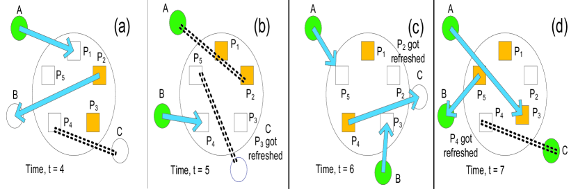
Figure 1: A schematic diagram showing the information dissemination process running in a DTN. Parts (a), (b), (c) and (d) show the status of the system at the beginning of the $4^{th}$, $5^{th}$, $6^{th}$ and $7^{th}$ time steps, in the process of dissemination. There are 5 places: $P_{1}$ … $P_{5}$ and 3 agents $A$,$B$,$C$ in the system. Each of the agents makes one visit to one of the places at every time step. We consider the dissemination of a single message only and hence, we consider that there is a buffer in each of the agents and the places which can hold a single message. The empty and the filled up circles (squares) denote agents (places) without or with the message in their buffers, respectively, at the specific annotated time step. As an agent makes a visit to a certain place, transfer of message happens only in the following two cases - (i) place has the message and the agent does not have it, or (ii) agent has the message but the place does not have it. The arrows denote the direction of transfer of the message. The dotted lines indicate that no message transfer took place. At the end of each time step, all the buffers are refreshed (message deleted) according to some probability value. The changes due to an operation performed in a particular time step is reflected in the next time step.

II-C Metrics

In our analysis, we use the two metrics as defined below to measure the efficiency of the dissemination process.

Agent coverage: The number of agents whose buffers contain the message that is being disseminated.

Place coverage: Given a message, the total number of throwboxes whose buffers receive and host the message (need not be simultaneously) due to the process of indirect dissemination described above.

In the small example depicted in figure 1, the agent coverage values at the $4^{th}$, $5^{th}$, $6^{th}$ and $7^{th}$ time steps are 1, 2, 2 and 3 respectively whereas the place coverage values at these time steps are 2, 2, 2 and 3 respectively. In this work, we mostly concentrate on the place coverage. However, we give an analysis of both of these metrics in section II-F.

There are two major issues associated with the described dissemination process. The first one is the agents’ mobility and the second one is the agents’ activity. In the next two subsections, we discuss the effect of both of these issues on the achieved coverage.

II-D Agents’ mobility

In this work the agents are considered to be only humans. In social context, preferential visit to different locations by humans has been the central idea of many proposed mobility models [25]. However, in order to keep it simple, in our analysis we consider the generalized version of the preferential selection process (complying with CMM) described as follows. At time step $t$, the chance that a place $P_{i}$ gets visited next by an agent, is modeled by the probability calculated through the following expression:

$$Prob(P_{i})=\frac{\left(d_{i}(t)+\delta\right)^{\alpha}}{\sum_{j=1}^{N}\left(d_{j}(t)+\delta\right)^{\alpha}}$$ (1)

where $d_{i}(t)$ reflects the number of agents that have already visited the place $P_{i}$ by time $t$ (i.e., the preference factor associated with a place); the parameter $\alpha$ is the clustering exponent [22]. In order to separately study the effect of the existing randomness (that moderates the preference factor) in the mobility of the agents, we introduce a parameter $\delta$ ($\geq 0$). We also assume that the stay times of the agents in the places are high and hence we ignore the transition time taken by an agent to jump from one place to the other [12].

However, in order to focus on the more fundamental properties of the dissemination process, we mostly consider $\delta$ = 0, and $\alpha$ = 1 for which the system reduces to a pure preferential one. Later, in section IV we discuss the effects of the non-zero values of $\delta$ and $\alpha$.

II-E Agents’ activity

From a global perspective, it may seem that some visits by different agents in the system take place simultaneously, i.e., at the same time. However, a more granular observation of the events reveal the fact that the probability that two distinct visits by two distinct agents to two different places or even at a same place happening exactly at the same time, is very low. In other words, at micro level timescales it is possible to perfectly order the events one after the other. Hence, without loss of generality, we assume that the agent’s visits happen sequentially and hence can be serialized according to the time stamps of those visits. This serializability of the sequence of agent visits allows us to rearrange them in a desired fashion whereby at each time step it is assumed that there is exactly one agent visit. We, however, assume that always the first agent in the system brings the message to be disseminated.

The duration of time that an agent actively participates in the dissemination process by visiting various places, can be termed as its life span (in other words, it is the time gap between the agent’s first visit and his last visit). These life spans of different agents may overlap with each other. The degree of this overlap can be controlled by restricting the life spans of the individual agents on the time line. In an extreme case of this spectrum, we have a fully overlapping model of the agent’s activity where the life spans of the agents may arbitrarily overlap with each other. In other words, if we consider the total period of activity as $T$, then in the said extreme case, an agent (say $n$) potentially stays active for the time span $E_{n}$ to $T$, where $E_{n}$ is the entry time of the agent $n$. The other extreme case is the model where the life spans of all the agents are fully disjoint from each other that is the total period of the activity of an agent is $E_{n}$ to $E_{n}+\mu-1$ where $\mu$ is the number of places visited by it. In between these two cases, we can appropriately restrict the life spans of the agents to reflect the cases where the life spans partially overlap with each other. These two scenarios of agents’ life span are pictorially explained in figure 2.

An important aspect to observe is the difference in performance arising due to varying degree of overlap. To check the difference, we empirically compare the time evolution of the achieved coverage under the two extreme cases of agents’ activity - fully overlapping and fully disjoint. To make a fair comparison, we assume that at each time step, in both the cases, $\mu$ distinct visits take place. Figure 3 shows the results for various combinations of $N$ and $\mu$. In all the cases, we find that for a given refresh probability ($p$), the coverage gets stabilized to a same value after a certain number of visits (initial delay) have been completed by the agents. The initial delay to reach the stability is much higher in the overlapping case. However, the significant observation obtained through experimentation is that the overlaps in the life spans of the agents do not have any specific effect on the final calculation of place coverage.

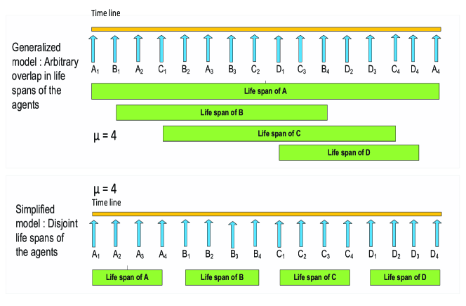
Figure 2: Disjoint and overlapping life spans of the agents. Four agents have been considered which are denoted by - A, B, C and D. Each agent is assumed to visit 4 places in the system (i.e., $\mu$=4). The subscript $i$ after an agent $X$ denotes the $i^{th}$ visit by the agent $X$. Part (a) shows the most general case where the life spans of the agents are overlapping with each other. Potentially any agent could have been active till the end. Part (b) shows the case where the life spans are all disjoint with each other.

We find that the final stabilized place coverage achieved in the dissemination process solely depends on the system parameters $N$, $\mu$ and the applied value of $p$. Hence, we concentrate only on this stabilized value of the coverage and its relationship with the other parameters. In order to get rid of the additional complexities due to the overlaps in the life spans of the agents, we adopt a simplified strategy described as follows. We assume that the life spans of the agents are disjoint. We also assume that each of the agents enters one by one, makes $\mu$ number of visits to different places and exits the system. This parameter $\mu$ actually models the average social participation of the agents. Here we have taken it as a constant but, analytically it can be shown [10] that the results remain same if it is assumed to be the average of the distribution of the number of visits an agent makes in its whole life span. Moreover, exploiting this simplistic setup we also safely assume that the dynamical time of the system is advanced after each individual agent completes all its $\mu$ visits as well as the buffers are refreshed (with probability $p$) at the end of every time unit.

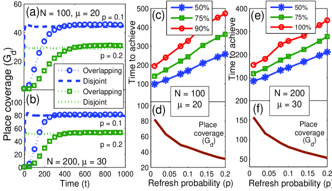
Figure 3: Parts (a) and (b) show the time evolution of the achieved coverage in the simulation of the dissemination process under overlapping and disjoint life spans of the agents for two different refresh probabilities and two different combinations of $N$ and $\mu$. Parts (c) and (e) show the plot of the relationship of the time to achieve a certain percentage of agent coverage with the applied refresh probability $p$ for two different combinations of $N$ and $\mu$. Parts (d) and (f) show the plot of the achieved place coverage for the refresh probabilities used in parts (c) and (e), respectively. In all these simulations, number of agents has been assumed to be 1000 and the results shown are the average over 1000 runs.

II-F Place coverage versus agent coverage

It should be noted that, for the sake of simplicity, in this analysis unlike the place buffers we do not consider any refreshing / resetting of the agents’ buffers. Therefore, with time the agent coverage gradually increases and after a certain time, all the agents that participate in the dissemination process get the message. Hence, the more important metric is to check the time needed to cover all the agents. We have already observed that place coverage decreases with the enhancement of refresh probability (figures 3 (a) and (b), also (d) and (f)). Figures 3 (c) and (e) show the relationship between the time to achieve a few different percentage of agent coverage with the applied refresh probability. The effect of the refresh probabilities is clearly visible - for higher values of the refresh probability, the time it takes to achieve a certain percentage of agent coverage is also high. Hence higher place coverage directly implies faster agent coverage. Thus, considering the importance of this place coverage, we set it to be the prime target of all the analysis presented in this paper. In the rest of this paper, we use the word ‘coverage’ to implicitly refer to this ‘place coverage’ (‘agent coverage’ is explicitly mentioned). We denote this quantity by $G_{d}$.

II-G Real data analysis

We use few publicly available GPS traces [33] to test whether the empirically observed temporal stability in coverage, also appears in real situation. In order to test this hypothesis the GPS trace needed to be appropriately processed which is elaborated next.

Data processing: These GPS trace data contain the information of the visits of a small number of agents at different places at different times within a certain campus area. However, the data of agent’s movement were of different days making it very sparse. Assuming regular pattern of activity where a trace in day $x$ would also appear in day $y$, we considered the trace record of a given agent for different days to be the records of separate agents. We subsequently merged all the trace records (of all the agents) together producing a consolidated trace record of a single day. We create equi-sized circles around different trace points and term the circular zones as places. We ignore the consecutive visits within same circle by the same agent. However, if an agent comes back to within a certain circle after visiting at least one different circle, we consider it to be a distinct visit. After obtaining all the visit points, we sort these common places in a descending order according to the number of visits to the places by different agents. To extract out the most popular places, we take only the top 20 places from this sorted list. This way we prepare four different datasets - KAIST, NC State fair, New York and NCSU (for details of the datasets, please see [33]).

Experiment: We run the dissemination algorithm already described on these processed datasets. We assume the existence of the message buffers (throwboxes) in the common places. We do the refreshing of the buffers and measure the coverage after the completion of every $k$ number of distinct visits by the agents. The value of $k$ is determined for each dataset depending on the total temporal length (number of hours) of the dataset as well as the frequency of the agent visits. For KAIST, NC State fair, New York and NCSU the values of $k$ are 50, 10, 4 and 4, respectively.

Results: The results are presented in figure 4. It can be observed from all these results that, for almost all different refresh probabilities the achieved coverage gets stabilized after a certain initial number of visits by the agents are over. To conclude, such stabilization is universal and is not an artifact of artificial systems. Hence, understanding the basic reason for this stabilization is an important step towards understanding the coverage dynamics.

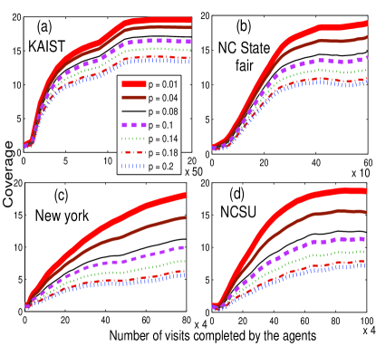
Figure 4: Plot of the coverage achieved by the application of message buffer in the information dissemination process implemented on four real datasets (a) KAIST, (b) NC State fair, (c) New York and (d) NCSU. The shown results are the average over 1000 runs of simulation of the dissemination process.

II-H Modeling with bipartite networks (BNW)

A natural and obvious interpretation of the underlying structure of DTN is a bipartite network where one partition (set of popular / common places) remains fixed in size over time and the other partition (set of agents and their visits) grows over time. Recent studies on BNW, such as [10, 11], have termed this kind of structure as $\alpha$-BiN. These works reveal few time invariant properties of such kind of BNWs. Being motivated by these works, we hypothesize that $\alpha$-BiN can be the ideal candidate to explain the stabilization of the place coverage ($G_{d}$) achieved in the DTN settings. To investigate further in this direction, we first formally model DTN as a BNW. We precisely establish a one-to-one mapping of the quantity which has to be analyzed in the DTN domain, as a quantity in the BNW domain. We briefly describe these techniques in the next section.

III $\alpha$-BiN and its relationship with DTN

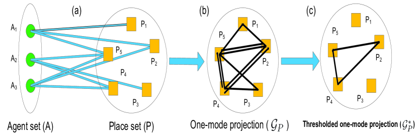
Figure 5: A schematic diagram of a possible scenario of the BNW corresponding to a DTN comprising five places, i.e., $N$=5 ($P_{1}$…$P_{5}$) and three agents, i.e., $t$=3 ($A_{1}$ … $A_{3}$) with $\mu$=3. The diagram shows a possible status after all the agents have joined the system. Part (a) shows the BNW, (b) is the one-mode projection and (c) is the thresholded one-mode projection for threshold value 2.

In order to establish the relationship between $\alpha$-BiN and DTN, several basic terminologies need to be defined which is done next. We then establish the correspondence.

III-A $\alpha$-BiN and its thresholded projection

As mentioned, $\alpha$-BiN is a bi-partite network where one partition (the place partition) is fixed and finite while the number of agents (the other partition) grows over time and is modeled by the parameter $t$. At any time instant $t$, an agent joins $\alpha$-BiN with $\mu$ connections where the connections are chosen preferentially (see figure 5). This can be thought of as the DTN situation where the life spans of the agents are disjoint and each agent makes connection sequentially one by one.

One-mode projection of the fixed partition (place set) is a place to place (weighted) graph where two places are connected by an edge if there is one common agent who visited/connected both of the places. We denote this structure by ${\mathcal{G}}_{P}$. The weight of an edge between two places in this projection denotes the number of parallel edges between the two places via same or different agents (see figure 5(b)).

Thresholded one-mode projection, is a simple graph derived from ${\mathcal{G}}_{P}$ where the edges whose weights fall below a certain threshold value $c$ in ${\mathcal{G}}_{P}$ are pruned out. We denote this construction by ${\mathcal{G}}_{P}^{*}$ (see figure 5(c)).

Time varying threshold: In general the value of the threshold $c$, can be taken to be a constant. But, it is apparent that as time grows (i.e., as more agents join the system), the structure ${\mathcal{G}}_{P}$ constructed from the $\alpha$-BiN gradually becomes a complete (weighted) graph. Thus, for a constant threshold, the corresponding ${\mathcal{G}}_{P}^{*}$ also becomes a complete (un-weighted) graph for sufficient growth of the $\alpha$-BiN. However, it has been shown in [11] that, instead of taking constant value, if the threshold value is computed by multiplying the number of agents joining the system (i.e., $t$) by a constant (say $v$, may be fraction also), i.e. $v~{}\times~{}t$, then certain properties of the resulting structure ${\mathcal{G}}_{P}^{*}$ converge and become time invariant, for a given value of $v$. We call this special kind of threshold value $v$ as time varying threshold.

Degree distribution in $\mathcal{G}_{P}^{*}$: The work [10] shows that the preferential growth of an $\alpha$-BiN can be understood as a variant of the well known Pólya urn model. Exploiting the exchangeability property of this Pólya urn model and applying de Finetti s theorem, they show that a single realization of the evolution of an $\alpha$-BiN can be mathematically understood in two steps - (a) first, a parameter, sampled from a Dirichlet distribution is preassigned with each of the place nodes in the fixed partition. We call this preassigned parameters as the attractiveness parameters and denote it by $\theta_{i}$ for node $i$. (b) Next, the agents are assumed to select a place node $i$ through a Bernoulli process with success rate equal to the attractiveness of $i$. The marginal distribution of the attractiveness parameters is a beta distribution. For special initial condition where all place nodes have equal degree 1, this beta distribution has the parameter set (1, $N$-1).

Furthermore, based on the above results, the authors in [11] derive that the growth rate of the weight of the edges between two nodes $i$ and $j$ in the one-mode projection of such $\alpha$-BiN, is asymptotically equal to the product of $\theta_{i}$ and $\theta_{j}$ and $(\mu_{2}-\mu)$, i.e.,

$$\lim_{t\to\infty}\frac{{W}(i,j)}{t}=(\mu_{2}-\mu)~{}\theta_{i}\theta_{j}$$ (2)

where $\theta_{i}$ and $\theta_{j}$ are the values of the attractiveness parameters associated with nodes $i$ and $j$, respectively; $W(i,j)$ is the weight of the edge between nodes $i$ and $j$ and $\mu$ and $\mu_{2}$ are the first and second moments of the distribution of the number of edges created by the nodes entering the growing set $V$.

The degree of a place node $i$ in $\mathcal{G}_{P}^{*}$ for a threshold value $c$ (= $v\times t$, at time $t$) will be the number of edges that are connected with $i$ in ${\mathcal{G}}_{P}$ and have weights larger equal $c$. Thus, exploiting equation 2, the work [11] also derives the cumulative degree distribution ($F_{v}(k)$) of $\mathcal{G}_{P}^{*}$ for a given time-varying threshold $v$ as follows -

$$F_{v}(k)=\left(1-\frac{v}{(\mu^{2}-\mu)x}\right)^{(N-1)},x=1-\left(\frac{k}{N-1}\right)^{\frac{1}{N-1}}$$ (3)

Special property of ${\mathcal{G}}_{P}^{*}$: A thresholded projection generally consists of a number of components (see figure 5). However, in case of a preferentially grown $\alpha$-BiN, due to a special distribution of the weights of the edges in ${\mathcal{G}}_{P}$, an interesting property is observed in the component structure of ${\mathcal{G}}_{P}^{*}$. This property relates the degree distribution of ${\mathcal{G}}_{P}^{*}$ and its largest component size. It (the property) is based on the following lemma.

Lemma $C$: The nodes which are in the largest component in $\mathcal{G}_{P}^{*}$ have strictly higher degree in $\mathcal{G}$ than the nodes which are outside the largest component in $\mathcal{G}_{P}^{*}$.

Argument: In the work [10], it has been derived that the expected degree of a node $i$ ($e(i)$) of set $P$ in $\mathcal{G}_{P}^{*}$ is equal to

$$(N-1)\left(1-\frac{v}{(\mu_{2}-\mu)\theta_{i}}\right)^{(N-1)}$$ (4)

where $v$ is the applied time varying threshold, $\theta_{i}$  is the probability that an agent will connect to node $i$ (in [10], this has been defined as the attractiveness of node $i$) and $\mu$, $\mu_{2}$ are respectively, the first and the second moments of the distribution of the number of edges created by the agent nodes entering the set $A$. Let us consider two nodes $i$ and $j$, where node $i$ has higher degree in $\mathcal{G}_{P}^{*}$ than node $j$, i.e., $e(i)>e(j)$. Using result 4, we can write that

$$(N-1)\left(1-\frac{v}{(\mu_{2}-\mu)\theta_{i}}\right)^{(N-1)}>$$

$$(N-1)\left(1-\frac{v}{(\mu_{2}-\mu)\theta_{j}}\right)^{(N-1)}$$

Manipulating this inequality, it can be easily proved that $\theta_{i}>\theta_{j}$. This implies, if a node $i~{}\epsilon~{}P$ has smaller degree than some other node $j~{}\epsilon~{}P$ in $\mathcal{G}_{P}^{*}$, then the attractiveness of node $i$ is lower than that of node $j$ (in $\mathcal{G}$). This attractiveness of a node $i$ ($\theta_{i}$), is a property of the BNW $\mathcal{G}$ and is directly proportional to the degree of $i$ in $\mathcal{G}$ (i.e., depends on how many agent’s connection a node could attract to itself in the past). Now, since we assume that at $t$=$T$, the nodes outside the largest component in $\mathcal{G}_{P}^{*}$ are degenerate, it simply follows that the nodes inside the component have higher degree in the BNW $\mathcal{G}$ itself (by virtue of having higher degree in $\mathcal{G}_{P}^{*}$) than the nodes outside the component. This proves the claim. $\diamond$

In the following we present the special property in the form of a theorem.

Theorem : For any given threshold value $v$, with high probability, the thresholded one-mode projection of a preferentially grown $\alpha$-BiN, contains a single connected component and all other nodes remain in the degenerate state.

Implication of the theorem: The property indicates a specific structure of the thresholded one-mode projection of a preferentially grown $\alpha$-BiN. This property also relates the number of components and the size of the largest component in $\mathcal{G}_{P}^{*}$ as follows. For any threshold value $v$, if the number of components in the thresholded one-mode projection, is ($C_{v}$) and the size (i.e., number of nodes) of the largest connected component is ($G_{b}$), then with high probability, $C_{v}$ + $G_{b}$ = $N$ + 1. where $N$ is the total number of nodes in the graph.

The proof follows.

Proof: Let us consider the $\alpha$-BiN $\mathcal{G}$ with set of agents $A$ and the set of places $P$. Recall that the one-mode projection on the place set is $\mathcal{G}_{P}$ and the thresholded one mode projection is $\mathcal{G}_{P}^{*}$.

Base condition: For $t$=0, i.e., when no agent has joined the system, the thresholded one mode projection will contain $N$ isolated nodes. Therefore, the theorem is trivially valid.

Induction hypotheses: We assume that for $t$=$T$, the thresholded one mode projection satisfies the theorem.

Induction step: We now prove that the theorem still holds true (with high probability) when agent number $t$=$T$+1 completes all its connections.

As the theorem is satisfied for $t$=$T$, we can say that after $T$ agents have joined the system, in $\mathcal{G}_{P}^{*}$, there is a single connected component of size less or equal to $N$ and the other nodes are isolated with degree zero.

Let us consider that the $(T+1)^{th}$ agent joins and creates $\mu$ number of connections. Let us focus on two subsets of the nodes from set $P$ in $\mathcal{G}_{P}^{*}$ at this instant of time. One subset ($S_{1}$) contains all the nodes with degree $u$ (in $\mathcal{G}$) and they currently reside inside the largest component and the other subset ($S_{2}$) contains the nodes outside the largest component comprising all the nodes of degree $v$ (in $\mathcal{G}$) (from the Claim $C$, it can be very easily proved that if some node of degree $d$ is outside the largest component, then all other nodes with the same degree are also outside the largest component. Similarly, the same is true for the degrees of the nodes inside the largest component).

We denote the probability that a randomly selected node is of degree $u$ and $v$ by $p_{u}$ and $p_{v}$ respectively. Therefore, the number of nodes of degree $u$ and $v$, i.e., the cardinality of the subset $S_{1}$ and $S_{2}$ are $Np_{u}$ and $Np_{v}$ respectively. As already $T$ agents have joined the system, the probability that the $(T+1)^{th}$ agent will select a $u$ degree node is $\frac{u}{T}$ (due to fully preferential selection). Therefore, out of $\mu$ connections of the $(T+1)^{th}$ agent, $\frac{u\mu}{T}Np_{u}$ connections will be towards the subset $S_{1}$ and similarly $\frac{v\mu}{T}Np_{v}$ connections will be towards the subset $S_{2}$.

Now, we consider three subsets of edges in the $\mathcal{G}_{P}$: $E_{1}$, $E_{2}$ and $E_{3}$. An element of set $E_{1}$ connects two nodes both of which are element of subset $S_{1}$ (i.e., connects two nodes both of which are inside the largest component). An element of set $E_{2}$ connects two nodes where one is in subset $S_{1}$ and the other is in subset $S_{2}$ (i.e., connects elements one from within and one outside the largest connected component). The elements of set $E_{3}$ connects two elements both of which are elements of the subset $S_{2}$ (i.e., connects two elements outside the largest component). The maximum number of elements possible in $E_{1}$, $E_{2}$ and $E_{3}$ are respectively $\binom{Np_{u}}{2}$,$Np_{u}\times Np_{v}$ and $\binom{Np_{v}}{2}$. These maximum number of possible edges can be thought as holes where edges which are newly created due to the joining of $(T+1)^{th}$ agent, get uniformly distributed. As a result of creating $\frac{u\mu}{T}Np_{u}$ and $\frac{v\mu}{T}Np_{v}$ edges by the $(T+1)^{th}$ agent, with the elements of the subset $S_{1}$ and $S_{2}$ respectively (in $\mathcal{G}$), the number of edges that will be created in $\mathcal{G}_{P}$ are $\binom{\frac{u\mu Np_{u}}{T}}{2}$, $\frac{u\mu Np_{u}}{T}\times\frac{v\mu Np_{v}}{T}$ and $\binom{\frac{v\mu Np_{v}}{T}}{2}$ respectively (assuming a node of $A$ creates at maximum one connection to a node of $P$). Therefore, the rate of increment of the weights of the edges of the elements forming the subset $E_{1}$, $E_{2}$ and $E_{3}$ are respectively $\frac{\binom{\frac{u\mu Np_{u}}{T}}{2}}{\binom{Np_{u}}{2}}$, $\frac{\frac{u\mu Np_{u}}{T}\times\frac{v\mu Np_{v}}{T}}{Np_{u}\times Np_{v}}$ and $\frac{\binom{\frac{v\mu Np_{v}}{T}}{2}}{\binom{Np_{v}}{2}}$. Let us denote these quantities as $r_{1}$, $r_{2}$ and $r_{3}$ respectively. Simplifying these rates we get $r_{1}$ is $\mathcal{O}(u^{2})$, $r_{2}$ is $\mathcal{O}(uv)$ and $r_{3}$ is $\mathcal{O}(v^{2})$.

Using the claim $C$, we can say that $u>v$ because, the nodes of $S_{1}$ are inside the largest component and the nodes of set $S_{2}$ are outside the largest component. Comparing the rates with each other, the following strictly descending order is obtained : $r_{1}>r_{2}>r_{3}$.

From this order we can conclude that the edges in $\mathcal{G}_{P}$ can be arranged in a strictly descending order (with high probability) in the following way based on the rate of increment of their weights: edges connecting two nodes both of which are inside the largest component, edges connecting two nodes exactly one of which is in the largest component, edges connecting nodes both of which are isolated. Therefore, with high probability, those edges which connect two nodes - one outside and another inside the largest component, will cross the threshold weight sooner than the edges which connect two nodes both of which are outside the largest component. As a result, the theorem still holds true after the $(T+1)^{th}$ agent completes its connections (with high probability). $\diamond$

Figure 6 shows a possible situation in the evolution process of the BNW when 9 agents have already joined the system, a single large component has already been formed and the $10^{th}$ agent joins.

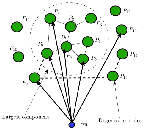
Figure 6: Schematic diagram of a possible situation at the $10^{th}$ time step in the evolution process in a BNW ($\mathcal{G}$) when $10^{th}$ agent joins the system. Place $P_{1}$…$P_{8}$ have already formed the single large component (encapsulated by dashed circle) and the rest nodes $P_{9}$ to $P_{15}$ are in a degenerate condition in the $\mathcal{G}_{P}^{*}$. The solid lines show the connections after applying threshold (i.e., in $\mathcal{G}_{P}^{*}$) and the dashed lines show the edges before thresholding in the one mode projection (i.e., in $\mathcal{G}_{P}$). At time step $T$=10, agent node $A_{10}$ arrives and creates 6 connections with the nodes in the place set (the lines with arrow head shows these connections). Nodes $P_{1}$, $P_{8}$ and $P_{6}$ (inside the largest component) have degree 5 each and nodes $P_{9}$ and $P_{15}$ (outside the largest) have degree 2 each in $\mathcal{G}$. Now, putting the values of $u$, $v$, $T$ and $\mu$ as 5,2,10 and 6 respectively, in the corresponding expressions of the rates (derived in the proof), it can be calculated that (approximately) $r_{1}$=9, $r_{2}$=3.6 and $r_{3}$=1.44. Hence, with high probability, the edge connecting $P_{8}$ and $P_{9}$ in $\mathcal{G}_{P}$ (average edge weight increment rate is 3.6 per agent) will acquire enough weight to cross the threshold weight much earlier than the edge connecting $P_{9}$ and $P_{15}$ (average edge weight increment rate is 1.44) and therefore, formation of a separate component does not occur and thus, with high probability the theorem still holds true after agent node $A_{10}$ completes all its connections.

Size of the largest component: Exploiting this property we calculate the size of the largest connected component of ${\mathcal{G}}_{P}^{*}$ as the fraction of the nodes having degree larger or equal to 1. We arrive at this quantity from the cumulative degree distribution of $\mathcal{G}_{P}^{*}$ (equation 3) as follows -

$$G_{b}=N\times\left[1-\left(\frac{\sqrt[N-1]{(N-1)}}{\sqrt[N-1]{(N-1)}-1}\right)\times\left(\frac{v}{\mu^{2}-\mu}\right)\right]^{N-1}$$ (5)

It can be inferred from [11], that the $F_{v}(k)$, for a given value of $v$ also bears time-invariant characteristics. $G_{b}$ is directly calculated from $F_{v}(k)$, hence is also independent of $t$. It can be concluded that the $G_{b}$ converges to a specific value for a given value of $v$; in other words it becomes independent of the number of agents that joined the system.

III-B Correspondence between $\alpha$-BiN and DTN

In both the BNW as well as the DTN domain, the parameters $N$, $\mu$ and $t$ have the same significance. In the DTN setup, the flow of the message between two places is controlled by the applied refresh probability $p$. The higher the value of $p$, the lower is the probability that a message will effectively get conveyed between a pair of places. We model this refresh probability using the parameter $v$ of the BNW. Hence, we estimate the coverage of information dissemination achieved under a certain value of $p$, i.e., $G_{d}$ by calculating the size of the largest component of the ${\mathcal{G}}_{P}^{*}$ in the corresponding BNW.

The parameters of the DTN and their relationship with those of the BNW are summarized in table I.

TABLE I: Relationship between the parameters in DTN and the corresponding BNW

Type	DTN	BNW	Remarks
Parameters	Agents($t$)	Agent partition ($t$)	Growing
	Places($N$)	Place partition ($N$)	Fixed and finite
	Number of place an agent visits ($\mu$)	Number of connections an agent creates with different places ($\mu$)	Constant (can be taken from some specified distribution also)
	Buffer refresh probability ($p$)	Threshold varying with $t$, ($v$)
Observable	Number of places where the message could reach under the dissemination process ($G_{d}$)	Size of the largest component of the thresholded one-mode projection ($G_{b}$)	These quantities should match

It is apparent that the two key parameters $p$ and $v$ create a bridge between the two domains - DTN and BNW. Hence, we also focus on understanding the functional relationship between $v$ and $p$.

Empirical validation: We simulate the time evolution of both $G_{d}$ as well as $G_{b}$ for many different parameter combinations. Figure 7 shows few such sample cases for different combinations of the other two parameters $N$ and $\mu$. It can be seen that the time series of these two quantities perfectly overlap for different choices of $(v,p)$ pairs.

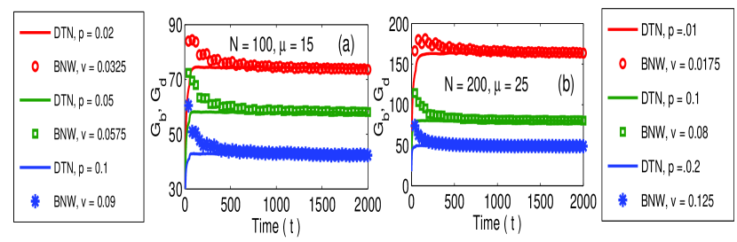
Figure 7: Comparison of the size of the largest component ($G_{b}$) in the thresholded one-mode projection of the BNW and the number of places in DTN where the message being disseminated is found, i.e., coverage ($G_{d}$). We consider the arrival of 2000 agents in both DTN and BNW. The two parts (a) and (b) of the figure show the results for two different combinations of $N$ and $\mu$. The results shown are the average over 100 runs of simulation.

Through experimentation we observe that, a linear relationship of the form $v=mp+c$, (where $m$ and $c$ are constants) exists in between $v$ and $p$. Figure 8 shows the comparison between the DTN simulation and the theoretical predictions from BNW. The theoretical results of BNW are derived in the following manner - at first, we derive the size of the giant component ($G_{b}$) for a whole range of $v$ value and then select that portion of the result (range of $v$) where the highest and the lowest value of $G_{b}$ perfectly overlap with the $G_{d}$ corresponding to the practical refresh probability ($p$) range (0.01 to 0.2). This portion is then plotted with the DTN result by linearly stretching the $v$ value to match the $p$ range. From the graph it is evident that just a linear transformation of $v$ value explains DTN coverage with high accuracy.

With this evidence, we now proceed to understand analytically the influence of various parameters on the performance of DTN (i.e., coverage).

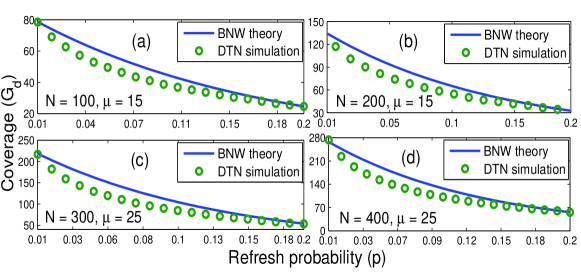
Figure 8: Comparison of the simulation of DTN and the theoretical predictions obtained from the corresponding BNW after proper linear re-scaling of the range of the values of $v$ and $p$. Different parts of the figure shows the same result for four different combinations of $N$and $\mu$. The results shown are the average over 100 runs of simulation.

IV Influence of the model parameters on coverage

In order to understand the role of the system parameters, we exploit the linear relationship between $p$ and $v$ - we replace $v$ by $p$ in equation 5, we also replace $G_{b}$ by $G_{d}$. Furthermore, using standard simplification techniques, the equation 5 changes to the following -

$$G_{d}=N-kN^{2}\frac{p(N-1)}{\mu(\mu-1)}$$ (6)

where $k$ is a constant.

In the following we present several significant insights drawn from the above mentioned simple formula.

IV-A Effect of the basic $\alpha$-BiN parameters

Effect of $p$ : For a certain fixed number of common places ($N$) and for a fixed number of visits ($\mu$) by the agents, the achieved coverage in DTN decreases linearly with the refresh probability. Figures 9(a) and (b) show few such sample results bringing out this linear relationship between the coverage and the $p$ (in the admissible range) for different choices of $N$ and $\mu$.

Effect of $N$: For a fixed number of visits by the agents and for a given refresh probability, the possibility of full coverage in DTN decreases at a rate proportional to the cubic power of the number of common places (i.e., $N^{3}$), that is, with the increase in size of $N$, it becomes very difficult to have full coverage. To illustrate this in figures 9(c) and (d), we plot the normalized coverage, that is, Coverage/$N$ in the y-axis. As seen in the graph, the coverage quickly diminishes with the increase in $N$.

Effect of $\mu$: For a certain fixed number of common places and for a given refresh probability, the achieved coverage in DTN increases at a rate proportional to $\mu^{2}$. Figure 9(e) presents few such sample results showing this relationship between $G_{d}$ and $\mu$. It can be seen from this figure that, up to a certain value of $\mu$, the achieved coverage $G_{d}$ increases rapidly (provided all other parameters remain fixed). However, beyond that, coverage hardly increases.

Furthermore, it can be shown that for a generalized distribution of the number of visits of the agents in the system (let us denote it by $F(x)$), the denominator ($\mu^{2}$ - $\mu$) in equation 6, can be replaced by ($\sigma^{2}+\psi(\psi-1))$ where $\psi$ and $\sigma$ are the average and the standard deviation of $F(x)$ (as shown in [10, 11]). Hence the inferences are (a) the achieved coverage only depends on the first and the second moment of $F(x)$ and (b) for a fixed value of $\psi$, if the number of agent visits are more diverse, (i.e., $F(x)$ has higher variance), then the achieved coverage in the dissemination process will be higher, i.e., the larger $F(x)$ varies, the higher is the coverage. Figure 9(f) presents few such results showing the relationship between the variance of $F(x)$ and the achieved coverage (detailed in the caption of the figure).

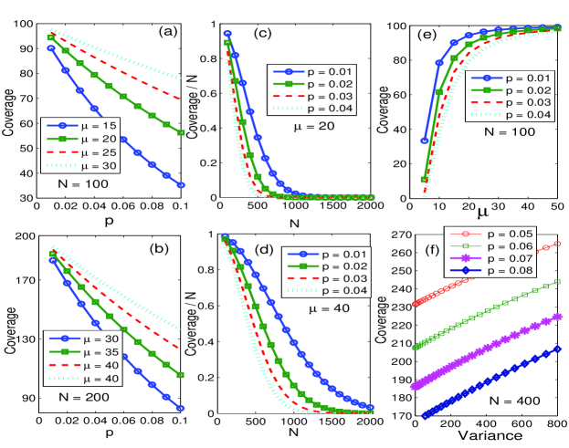
Figure 9: Parts (a) and (b) show the plot of the relationship between the refresh probability and the coverage in DTN, for different combinations $N$ and $\mu$. Parts (c) and (d) show dependence of the fraction of the nodes covered in DTN, i.e, $\frac{coverage}{N}$ on the total number of places for different combinations of $\mu$ and $p$. Part (e) shows the relationship between the coverage in DTN and $\mu$ for $N$=100 and different values of $p$. All these presented relationships are derived from equation 6. Part (f) shows the relationship between the coverage and the variance of the distribution of the number of places visited by the agents for $N$ = 1000 and few different values of the $p$. We consider an uniform distribution of the number of places visited by the agents. We set the value of average of this distribution (=$\mu$) at 50 and vary the range of the value (such as [1,99], [11, 89], [21,79] etc.) to vary the variance. For each different variance we calculate the achieved coverage from equation 6.

IV-B Effect of mobility related parameters

We also consider two other parameters related to the mobility of the agents - (a) randomness in selecting new places ($\delta$) (b) propensity of the agents to visit nearer places, termed as clustering exponent ($\alpha$). These two terms have been discussed in section II-D and equation 1.

Effect of randomness, $\delta$ : We find that the achieved coverage increases noticeably for the initial values of $\delta$ (between 0 and 1) and changes very slowly for higher values. Figures 10(a) to (d), show some sample results for few different combinations of $N$, $\mu$ and $p$. The reason for the improvement in coverage with the slight increase in the randomness is that with randomness, people tend to visit many other places with higher frequency in comparison to the pure preferential case.

Effect of clustering exponent, $\alpha$ : We observe completely opposite effect of $\alpha$ on the achieved coverage. We find a drastic decrease in $G_{d}$ with even a very small increase in the $\alpha$. Figures 10(e) to (h) show some sample results for few different combinations of $N$, $\mu$ and $p$. This happens due to the fact that, for higher value of $\alpha$, people tend to visit in a more clustered fashion, i.e., few places start getting visited even at higher frequencies while the other places get visited with lesser frequencies in comparison to the pure preferential case. Subsequently a super-preferential attachment dynamics emerges; hence the number of places preserving the message drastically decreases.

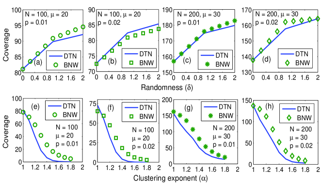
Figure 10: Parts (a) - (d) show the plot of the achieved coverage in the simulation of message dissemination in DTN, for several different values of $\delta$, under two different refresh probabilities and two different combinations of $N$ and $\mu$. Parts (e) - (h) show the plot of the achieved coverage in DTN, for several different values of $\alpha$, under two different refresh probabilities and two different combinations of $N$ and $\mu$. The simulation results obtained from the BNW have been also shown. All the simulation results were computed by averaging over 1000 runs.

V Related Work

Bipartite networks and their projections have been employed as a model in various diverse fields, e.g., personal recommendation [28, 41, 38], analysis of social networks [23, 31, 37], protein structures [24], linguistics [7] etc. In the current work we use an evolving bipartite network [10] to model the message dissemination process in buffer augmented DTN. On the other hand, the spreading processes also have been studied immensely using various models such as SI, SIS, SIR, SIRS [1, 18] etc. Even recently bipartite networks have been studied under such frameworks [14, 15]. However, message dissemination in DTN being a computer-science application specific problem, the place coverage as studied in this paper, is more significant in this context than various other critical issues which are generally analyzed in epidemiology. In the following we briefly describe the existing works in this specific direction.

In the communication network literature, from the perspective of information dissemination, the coverage, i.e., number of distinctly visited nodes in any network, has been a significant metric. Many works have been done on developing either efficient algorithms or analyzing the maximum achievable coverage [9, 20, 27, 29, 30] in both wired and wireless networks through appropriate modeling of the undergoing process. However, similar work for DTN (augmented with message buffers [40, 16]) is largely missing in the literature.

Most dissemination schemes proposed for DTN follow a store-carry-forward paradigm in which the mobile devices carried by the agents temporarily buffer the data and forward it to other (appropriate) agents. Various strategies like epidemic routing [36], spray and wait protocols [35], contact history-based protocols [4] have been employed to enhance the speed and amount of coverage. In addition, the efficiency of any such strategy heavily depends on exploiting the patterns emerging from the underlying mobility models. Various such models have been proposed - from the simple random walk [3] to the more sophisticated models such as self similar least action walk  [21].

A majority of the past studies assume a suitable mathematical abstraction of the real world DTN environment and observe the important characteristics through simulations and analytics. This is a very standard and well accepted approach adopted in the literature [36, 35] which has been also the central policy of the current work. Several stochastic techniques like epidemic spreading [8], ordinary differential equations [39], partial differential equations [6] as well as Markov models [2] have been applied to gain the necessary analytical insight. However, the use of store-carry-forward paradigm in the dissemination processes adopted for DTN in conjunction with the complex human mobility models, make it extremely difficult to produce neat results using such traditional mathematical tools. All the above mentioned works in the direction of analyzing coverage, either use very simplistic setup or ultimately land up in very complicated open equations where the relationships among the key parameters of the system cannot be easily understood from these equations. The work presented in this paper is significant in the sense that we come up with simple closed form equations through clever modelling of the complex process.

Recently, Gu et al [12] have addressed this issue in similar lines as those presented in this paper. They have perceived the use of message buffers as an instance of bio-inspired methods (e.g., pheromone or footprint). Using discrete Markov chain based modeling, they analyzed the importance of buffer time as well as the preferences of visiting different places by the mobile agents. They studied the impact of these two crucial system features on the latency and the message delivery ratio of the dissemination process in the network. In our work, we specifically emphasize on the inherent bipartite nature of the “throwbox augmented DTN” and thus bring forward the fact that instead of starting from scratch, the existing theories of the bipartite network can be used (with necessary modifications) to analyze the coverage problems related to DTN. In [34] we introduced this methodology for the first time and reported certain initial results. The settings assumed there have been largely artificial where neither real-life traces, clustered mobility models etc. have been considered. We also assumed theoretical setups like buffer time, i.e., the number of time steps for which a given message is stored in a message buffer (denoted by $b$), to be a globally fixed quantity. However, here we adopt the buffer refresh probability which happens to be more easily implementable (hence practical), maintainable and cost effective solution. Moreover, we also demonstrate here our detailed study on how the coverage in DTN gets affected depending on various issues related to the mobility of the agents -like their life spans, activities, variation in the place selection strategy.

VI Conclusion

In this work we introduce a new mathematical tool (bipartite network) to analyze place coverage in the process of information dissemination through indirect message transfer in DTN. We show that the size of the largest component of the thresholded projection of an appropriately constructed bipartite network, can be used to accurately measure place coverage. We also demonstrate a straightforward way of calculating the size of the largest component from the degree distribution. Moreover, from the mathematical equations we derive several simple insights regarding the complex process of message spreading in throwbox augmented DTN. One of the most significant non-intuitive results is that place coverage converges and does not increase beyond a certain level for a given refresh probability ($p$) and this level is significantly lower than full coverage for even a very small value of $p$. The lesson learned is that if the number of places increases or the variation of agent activity is not very high or if the agents have the tendency to roam within only popular places, even the introduction of throwbox as a backbone infrastructure may not be sufficient.

References

- [1] R. Anderson and R. M. May, Infectious diseases of humans: Dynamics and control. Oxford: Oxford University Press, 1992.
- [2] C. Boldrini, M. Conti, and A. Passarella, “Modelling data dissemination in opportunistic networks,” in Proceedings of the third ACM workshop on Challenged Networks, ser. CHANTS ’08. New York, NY, USA: ACM, 2008, pp. 89–96. [Online]. Available: http://doi.acm.org/10.1145/1409985.1410002
- [3] J. Broch, D. A. Maltz, D. B. Johnson, Y.-C. Hu, and J. Jetcheva, “A performance comparison of multi-hop wireless ad hoc network routing protocols,” in Proceedings of the 4th annual ACM/IEEE international conference on Mobile computing and networking, ser. MobiCom ’98. New York, NY, USA: ACM, 1998, pp. 85–97. [Online]. Available: http://doi.acm.org/10.1145/288235.288256
- [4] J. Burgess, B. Gallagher, D. Jensen, and B. N. Levine, “MaxProp: Routing for Vehicle-Based Disruption-Tolerant Networks,” in Proceedings IEEE INFOCOM, Apr. 2006. [Online]. Available: http://prisms.cs.umass.edu/brian/pubs/burgess.infocom2006.pdf
- [5] E. Burgos, H. Ceva, L. Hernández, R. P. J. Perazzo, M. Devoto, and D. Medan, “Two classes of bipartite networks: Nested biological and social systems,” Phys. Rev. E, vol. 78, p. 046113, Oct 2008. [Online]. Available: http://link.aps.org/doi/10.1103/PhysRevE.78.046113
- [6] A. Chaintreau, J.-Y. Le Boudec, and N. Ristanovic, “The age of gossip: spatial mean field regime,” in Proceedings of SIGMETRICS ’09: the eleventh international joint conference on Measurement and modeling of computer systems. New York, NY, USA: ACM Press, June 2009, pp. 109–120. [Online]. Available: http://dx.doi.org/10.1145/1555349.1555363
- [7] M. Choudhury, N. Ganguly, A. Maiti, A. Mukherjee, L. Brusch, A. Deutsch, and F. Peruani, “Modeling discrete combinatorial systems as alphabetic bipartite networks: Theory and applications,” Phys. Rev. E, vol. 81, p. 036103, Mar 2010. [Online]. Available: http://link.aps.org/doi/10.1103/PhysRevE.81.036103
- [8] D. J. Daley and J. Gani, Epidemic Modelling: An Introduction (Cambridge Studies in Mathematical Biology), 1st ed. Cambridge University Press, May 2001. [Online]. Available: http://www.amazon.com/exec/obidos/redirect?tag=citeulike07-20“&path=ASI%N/0521014670
- [9] V. V. Dimakopoulos and E. Pitoura, “On the performance of flooding-based resource discovery,” IEEE Trans. Parallel Distrib. Syst., vol. 17, no. 11, pp. 1242–1252, Nov. 2006. [Online]. Available: http://dx.doi.org/10.1109/TPDS.2006.161
- [10] N. Ganguly, S. Ghosh, T. Krueger, and A. Srivastava, “Degree distributions of evolving alphabetic bipartite networks and their projections,” Theoretical Computer Science, vol. 466, no. 0, pp. 20 – 36, 2012. [Online]. Available: http://www.sciencedirect.com/science/article/pii/S0304397512007682
- [11] S. Ghosh, S. Saha, A. Srivastava, T. Krueger, N. Ganguly, and A. Mukherjee, “Understanding evolution of inter-group relationships using bipartite networks,” Selected Areas in Communications, IEEE Journal on, vol. PP, no. 99, pp. 1–11, 2013.
- [12] B. Gu, X. Hong, and P. Wang, “Analysis for bio-inspired thrown-box assisted message dissemination in delay tolerant networks,” Telecommun Syst, Springer, 2011.
- [13] J.-L. Guillaume and M. Latapy, “Bipartite structure of all complex networks,” Information processing letters, vol. 90, no. 5, pp. 215–221, 2004.
- [14] D. G. Hernández and S. Risau-Gusman, “Epidemic thresholds for bipartite networks,” Phys. Rev. E, vol. 88, p. 052801, Nov 2013. [Online]. Available: http://link.aps.org/doi/10.1103/PhysRevE.88.052801
- [15] X. Huang, I. Vodenska, S. Havlin, and H. E. Stanley, “Cascading failures in bi-partite graphs: model for systemic risk propagation,” Scientific reports, vol. 3, 2013.
- [16] M. Ibrahim, A. Al Hanbali, and P. Nain, “Delay and resource analysis in manets in presence of throwboxes,” Perform. Eval., vol. 64, no. 9-12, pp. 933–947, Oct. 2007. [Online]. Available: http://dx.doi.org/10.1016/j.peva.2007.06.005
- [17] J. Jaworski, M. Karoński, and D. Stark, “The degree of a typical vertex in generalized random intersection graph models,” Discrete Mathematics, vol. 306, no. 18, pp. 2152 – 2165, 2006. [Online]. Available: http://www.sciencedirect.com/science/article/pii/S0012365X0600361X
- [18] M. J. Keeling and P. Rohani, Modeling infectious diseases in humans and animals. Princeton University Press, 2008.
- [19] M. Kitsak and D. Krioukov, “Hidden variables in bipartite networks,” Phys. Rev. E, vol. 84, p. 026114, Aug 2011. [Online]. Available: http://link.aps.org/doi/10.1103/PhysRevE.84.026114
- [20] H. Larralde, P. Trunfio, S. Havlin, H. E. Stanley, and G. H. Weiss, “Number of distinct sites visited by N random walkers,” Phys. Rev. A, vol. 45, pp. 7128–7138, May 1992. [Online]. Available: http://link.aps.org/doi/10.1103/PhysRevA.45.7128
- [21] K. Lee, S. Hong, S. J. Kim, I. Rhee, and S. Chong, “Slaw: A new mobility model for human walks,” in INFOCOM 2009, IEEE, April 2009, pp. 855–863.
- [22] S. Lim, C. Yu, and C. Das, “Clustered mobility model for scale-free wireless networks,” in Local Computer Networks, Proceedings 2006 31st IEEE Conference on, 2006, pp. 231–238.
- [23] J.-G. Liu, Z. Hu, and Q. Guo, “Effect of the social influence on topological properties of user-object bipartite networks,” The European Physical Journal B, vol. 86, no. 11, pp. 1–11, 2013.
- [24] S. Maslov and K. Sneppen, “Specificity and stability in topology of protein networks,” Science, vol. 296, no. 5569, pp. 910–913, 2002. [Online]. Available: http://www.sciencemag.org/content/296/5569/910.abstract
- [25] A. Mei and J. Stefa, “SWIM: A simple model to generate small mobile worlds,” in INFOCOM 2009, IEEE, 2009, pp. 2106–2113.
- [26] A. Mukherjee, M. Choudhury, and N. Ganguly, “Understanding how both the partitions of a bipartite network affect its one-mode projection,” Physica A, vol. 390, no. 20, pp. 3602 – 3607, 2011.
- [27] S. Nandi, L. Brusch, A. Deutsch, and N. Ganguly, “Coverage-maximization in networks under resource constraints,” Phys. Rev. E, vol. 81, p. 061124, Jun 2010. [Online]. Available: http://link.aps.org/doi/10.1103/PhysRevE.81.061124
- [28] D.-C. Nie, Y.-H. An, Q. Dong, Y. Fu, and T. Zhou, “Information filtering via balanced diffusion on bipartite networks,” arXiv preprint arXiv:1402.5774, 2014.
- [29] K. Oikonomou, D. Kogias, and I. Stavrakakis, “Probabilistic flooding for efficient information dissemination in random graph topologies,” Comput. Netw., vol. 54, no. 10, pp. 1615–1629, July 2010. [Online]. Available: http://dx.doi.org/10.1016/j.comnet.2010.01.007
- [30] K. Oikonomou and I. Stavrakakis, “Performance analysis of probabilistic flooding using random graphs,” in Proceedings of IEEE WOWMOM 2007, june 2007, pp. 1–6.
- [31] T. Opsahl, “Triadic closure in two-mode networks: Redefining the global and local clustering coefficients,” Social Networks, vol. 35, no. 2, pp. 159–167, 2013.
- [32] F. Peruani, M. Choudhury, A. Mukherjee, and N. Ganguly, “Emergence of a non-scaling degree distribution in bipartite networks: A numerical and analytical study,” EPL (Europhysics Letters), vol. 79, no. 2, p. 28001, 2007. [Online]. Available: http://stacks.iop.org/0295-5075/79/i=2/a=28001
- [33] I. Rhee, M. Shin, S. Hong, K. Lee, S. Kim, and S. Chong, “CRAWDAD data set ncsu/mobilitymodels (v. 2009-07-23),” Downloaded from http://crawdad.cs.dartmouth.edu/ncsu/mobilitymodels, July 2009.
- [34] S. Saha, N. Ganguly, and A. Mukherjee, “Information dissemination dynamics in delay tolerant network: a bipartite network approach,” in Proceedings of the third ACM international workshop on Mobile Opportunistic Networks, ser. MobiOpp ’12. New York, NY, USA: ACM, 2012, pp. 21–28. [Online]. Available: http://doi.acm.org/10.1145/2159576.2159583
- [35] P. U. Tournoux, J. Leguay, F. Benbadis, V. Conan, M. Dias de Amorim, and J. Whitbeck, “The Accordion phenomenon: Analysis, characterization, and impact on DTN routing,” in Proceedings of IEEE INFOCOM 2009 - The 28th Conference on Computer Communications. IEEE, Apr. 2009, pp. 1116–1124. [Online]. Available: http://dx.doi.org/10.1109/INFCOM.2009.5062024
- [36] A. Vahdat and D. Becker, “Epidemic Routing for Partially-Connected Ad Hoc Networks,” CS-200006, Duke University, Tech. Rep., Apr. 2000. [Online]. Available: http://issg.cs.duke.edu/epidemic/epidemic.pdf
- [37] M. Yu, K. Zhao, J. Yen, and D. Kreager, “Recommendation in reciprocal and bipartite social networks–a case study of online dating,” in Social Computing, Behavioral-Cultural Modeling and Prediction. Springer, 2013, pp. 231–239.
- [38] W. Zeng, A. Zeng, M.-S. Shang, and Y.-C. Zhang, “Information filtering in sparse online systems: recommendation via semi-local diffusion,” PloS one, vol. 8, no. 11, p. e79354, 2013.
- [39] X. Zhang, G. Neglia, J. Kurose, and D. Towsley, “Performance modeling of epidemic routing,” Comput. Netw., vol. 51, no. 10, pp. 2867–2891, July 2007. [Online]. Available: http://dx.doi.org/10.1016/j.comnet.2006.11.028
- [40] W. Zhao, Y. Chen, M. H. Ammar, M. D. Corner, B. N. Levine, and E. W. Zegura, “Capacity enhancement using throwboxes in dtns.” in Proceedings of MASS. IEEE, 2006, pp. 31–40.
- [41] T. Zhou, J. Ren, M. c. v. Medo, and Y.-C. Zhang, “Bipartite network projection and personal recommendation,” Phys. Rev. E, vol. 76, p. 046115, Oct 2007. [Online]. Available: http://link.aps.org/doi/10.1103/PhysRevE.76.046115