Solar cycle 25: another moderate cycle?

Abstract

Surface flux transport simulations for the descending phase of cycle 24 using random sources (emerging bipolar magnetic regions) with empirically determined scatter of their properties provide a prediction of the axial dipole moment during the upcoming activity minimum together with a realistic uncertainty range. The expectation value for the dipole moment around 2020 $(2.5\pm 1.1\,$G) is comparable to that observed at the end of cycle 23 (about $2\,$G). The empirical correlation between the dipole moment during solar minimum and the strength of the subsequent cycle thus suggests that cycle 25 will be of moderate amplitude, not much higher than that of the current cycle. However, the intrinsic uncertainty of such predictions resulting from the random scatter of the source properties is considerable and fundamentally limits the reliability with which such predictions can be made before activity minimum is reached.

1 Introduction

Owing to the growing practical importance of space weather, attempts to predict future levels of solar activity have found much interest in recent years. A considerable variety of methods has been suggested, of which the so-called precursor methods proved most successful (see review by Petrovay, 2010). These methods take the strength of the magnetic field at the solar polar caps (or some proxy thereof, such as the open heliospheric magnetic flux, the strength of the radial interplanetary field, or the level of geomagnetic disturbances) during activity minimum as indicator for the strength of the subsequent cycle. The high empirical correlation between precursor level and cycle strength (e.g. Wang & Sheeley, 2009) has a theoretical basis in the Babcock-Leighton scenario for the solar dynamo (Charbonneau, 2010; Cameron & Schüssler, 2015). Thus a prediction of the amplitude of the next activity maximum made at a time around minimum, when the polar fields are fully developed, rests on rather solid empirical and theoretical ground. The level of uncertainty of such a prediction can be estimated from the data.

The question is whether and how a prediction at an earlier phase during a cycle can be made. One possibility is to use surface flux transport (SFT) simulations, which have quite successfully reproduced the observed evolution of the large-scale magnetic field at the solar surface in the course of the solar cycle, particulary also the evolution of the polar fields and axial dipole moment (e.g. Wang et al., 1989; Sheeley, 2005; Mackay & Yeates, 2012; Jiang et al., 2014b; Upton & Hathaway, 2014). Such simulations also showed that randomness in the properties of the magnetic flux sources in the form of emerging bipolar magnetic regions (such as emergence latitude and tilt angle) has a strong effect: single bipolar regions emerging near the equator can significantly affect the level of the polar field (or axial dipole moment) around solar minimum and thus influence the strength of the subsequent cycle (Jiang et al., 2014a, 2015). Therefore, any prediction of the polar field strength also needs to quantify the uncertainty that arises from the random scatter of the source properties.

In the work presented in this paper, we used empirically determined statistical properties of emerging bipolar regions (sunspot groups) during the declining phases of solar cycles and ran Monte-Carlo ensembles of SFT simulations starting from observed synoptic maps of the surface magnetic field. We thus obtained the axial dipole moment during solar minima as an ensemble average over the realizations together with an empirically based estimate of the uncertainty. We prefer to consider the axial dipole moment and not the polar field strength since it is a uniquely defined quantity and limits the effect of a hemispherically asymmetric distribution of magnetic flux. Around activity minima, the axial dipole moment is dominated by the magnetic flux at the polar caps and represents the open heliospheric flux. We first tested our approach by deriving postdictions for the axial dipole moment during the minima of cycles 21-23, which can be compared with observations. We then ran simulations for cycle 24 and obtained predictions and statistical uncertainties for the dipole moment during the upcoming minimum around 2020.

2 Surface flux transport (SFT) model

2.1 SFT code

The SFT code used is described in Baumann et al. (2004) and Cameron et al. (2010). It treats the evolution of the radial component of the large-scale magnetic field at the solar surface resulting from passive transport by convection, differential rotation, and meridional flow. The corresponding magnetohydrodynamic induction equation is given by

$$\frac{\partial B}{\partial t}= -\Omega(\lambda)\frac{\partial B}{\partial\phi}-\frac{1}{R_{\odot}\cos\lambda}\frac{\partial}{\partial\lambda}[\upsilon(\lambda)B\cos\lambda]$$ (1)

$$+\eta\left[\frac{1}{R_{\odot}^{2}\cos{\lambda}}\frac{\partial}{\partial\lambda}\left(\cos\lambda\frac{\partial B}{\partial\lambda}\right)+\frac{1}{R_{\odot}^{2}\cos^{2}{\lambda}}\frac{\partial^{2}B}{\partial\phi^{2}}\right]+S(\lambda,\phi,t),$$

where $B(\lambda,\phi,t)$ is the radial component of the magnetic field. $\lambda$ and $\phi$ are heliographic latitude and longitude, respectively. We used the profile of latitudinal differential rotation, $\Omega(\lambda)$, determined by Snodgrass (1983) and took the profile of the poleward meridional flow, $\upsilon(\lambda)$, from van Ballegooijen et al. (1998). The magnetic diffusivity $\eta=250$ km²s^-1 describes the random walk of the magnetic flux elements as transported by supergranulation flows (Leighton, 1964). The source term, $S(\lambda,\phi,t)$, represents the emergence of magnetic flux at the solar surface. The properties of the corresponding bipolar regions were defined as described in Baumann et al. (2004). Further details are given in Cameron et al. (2010).

2.2 Source selection and initial condition

Our method requires us to provide synthetic source data (emerging bipolar magnetic regions, BMRs) for the time period of the prediction. The properties of these sources were chosen according to their empirical statistics during the descending phases of previous activity cycles.

The number of BMRs emerging per month of the simulation was taken to be equal to $R/2.75$, where $R$ is the monthly sunspot number. This calibration was carried out on the basis of the sunspot data for cycles 21–24 (between 1976 and 2016). We adopted the functional form $R_{G}=f(t)+\Delta f(t)$, where $f(t)$ is given by Eq. (1) of Hathaway et al. (1994) and $\Delta f(t)$ represents the random scatter of the time evolution. We followed the procedure given in Hathaway et al. (1994) to fix the independent parameters $a$ (amplitude) and $t_{0}$ (starting time) involved in $f(t)$ from observational data for the cycles considered here. The obtained values for $(a;t_{0})$ are $(0.00351;1976.39)$ for cycle 21, $(0.00336;1986.16)$ for cycle 22, $(0.00229;1996.57)$ for cycle 23, and $(0.00103;2008.84)$ for cycle 24. The standard deviation $\sigma_{f}(t)$ of $\Delta f(t)$ is determined from the difference between the fit profiles $f(t)$ and the observed profiles for cycles 21–23. It is well represented by $\sigma_{f}(t)=0.5f(t)$.

For the latitudinal distribution of the sources as a function of cycle phase we used the empirically derived functional forms for mean latitude and width (standard deviation, $\sigma_{\lambda}$) of the activity belts given by Eqs. (4) and (5) of Jiang et al. (2011). The area distribution for the emerging BMRs and its dependence on cycle phase follows the empirical profiles represented by Eqs. (12)–(14) of Jiang et al. (2011).

The mean tilt angle, $\alpha_{n}(\lambda)$, of the emerging BMRs for cycle number $n$ is assumed to follow Joy’s law in the form $\alpha_{n}(\lambda)=T_{n}\sqrt{|\lambda|}$. $T_{n}$ was taken from the linear relation with maximum sunspot number given by Eq. (15) of Jiang et al. (2011). For the scatter of the tilt angle, $\sigma_{\alpha}$ (in degrees), we used the empirical relation with sunspot umbral area, $A_{U}$, given by $\sigma_{\alpha}=-11\log A_{U}+35.$ as determined by Jiang et al. (2014a). To connect total sunspot area, $A_{S}$, and BMR area with umbral area, we used the relation $A_{S}=5A_{U}$ (Brandt et al., 1990).

The relevant quantity for the contribution of a BMR to the axial dipole moment is the latitudinal separation of the two polarities, which depends on the tilt angle and on the distance between the polarities. For the latter we employ its empirical relation with the BMR area as derived by Cameron et al. (2010). Here the BMR area is defined as the sum of sunspot area and plage area, using the relationship derived from observations by Chapman et al. (1997). The distribution of latitudinal polarity distance derived by this procedure agrees well with that determined directly from historical sunspot data. This applies particularly to the tails of the distribution, which are most important for the buildup of the polar fields.

The procedure for defining the sources is then as follows: for each month of the simulation, the number of emerging BMRs is determined according to the value of $f(t)$ and a random deviation $\Delta f(t)$. These BMRs are distributed randomly over the days of the month. For each emerging BMR, its size is chosen randomly from the (time-dependent) size distribution. Its latitude is given by the (time-dependent) mean latitude plus a random component drawn from a distribution with standard deviation $\sigma_{\lambda}$. The tilt angle is chosen according to Joy’s law plus a random component drawn from a distribution with standard deviation $\sigma_{\alpha}$. The resulting tilt angle is multiplied by a factor 0.7 to account for the effect of latitudinal inflows towards active regions (Cameron et al., 2010). Finally, the BMRs are distributed randomly over longitude and the two hemispheres.

The introduction of the factor 0.7 is neccessary because the tilt angle distributions empirically determined by Jiang et al. (2014a) refer to the instant of maximum sunspot area during the evolution of an active region, which typically is a few days after the beginning of flux emergence. Martin-Belda & Cameron (2016, see Fig. 8 therein) have shown that the lateral inflows towards active regions significantly reduce the tilt angle after this moment. Quantitatively, the reduction is consistent with the factor 0.7 assumed here, a value that also provided good reproduction of the observationally inferred polar fields (open heliospheric flux) during the activity minima between 1913 and 1986 with our flux transport model (Cameron et al., 2010).

Fig. 1 shows an example for one realization of random sources for cycle 24. The upper panel provides a comparison of the actual monthly group sunspot number (black), one realization of the random sources (red) and the average of 50 random realizations (blue). The lower panel shows a butterfly diagram with the actual sunspot groups (black crosses) and one realization of the random sources (red crosses).

We started the SFT simulations from observed synoptic magnetograms using data from NSO/KPVT (available from 8/1976 until 8/2003), NSO/SOLIS (8/2003 until present), SOHO/MDI (6/1996 until 11/2010), and SDO/HMI (5/2010 until present). All magnetogram data used were reduced to a resolution of $1\deg$ in latitude and longitude, respectively.

2.3 Error estimate

For a sensible prediction, we need to quantify the uncertainty involved in our extrapolation of the evolution of the axial dipole moment based on SFT simulations with random sources. Two causes of error are considered here: 1) uncertainty due to scatter in the properties of the source BMRs (number, emergence location, size, and tilt angle) and 2) uncertainty due to measurement error in the magnetogram used as initial state. While (1) represents the intrinsic uncertainty resulting from the random component of the solar dynamo process, the contribution of (2) is due to imperfect measurement and depends on the instrument that provided the data, the data analysis procedure, etc. Since both contributions to the total error are uncorrelated, they add quadratically.

The effect of the scatter in the source properties (1) was determined by repeating each SFT simulation 50 times with different random realizations of the sources. The uncertainty resulting from the error in the initial magnetograms (2) was estimated by consideing the averaged measured radial surface field,

$$\overline{B_{r}}(t)=\frac{1}{4\pi}\int_{\pi/2}^{-\pi/2}\int_{0}^{2\pi}B_{r}(\lambda,t)\cos\lambda d\lambda d\phi,$$ (2)

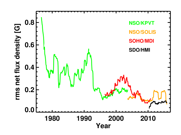
Figure 2: RMS fluctuation of the surface-averaged radial magnetic field shown by synoptic magnetograms. The line colors indicate the data source as indicated in the legend.

which should vanish since the magnetic field is divergence-free. Any deviation from zero must therefore be due to measurement error (e.g., instrumental noise, Zeeman saturation, $B$ angle correction). We estimate the rms error of $\overline{B_{r}}$ by considering a 19-month running mean (indicated by angular brackets), $\varepsilon(t)=\langle\overline{B_{r}}^{2}\rangle^{1/2}$. Fig. 2 shows $\varepsilon(t)$ for the various time series of synoptic magnetograms considered here. As the instruments were improved over time and became characterized better, $\varepsilon$ decreased since 1976 by about a factor of 10 from values over $0.8\,$G to about $0.08\,$G. In the estimate of the rms error we can safely neglect the average $\langle\overline{B_{r}}\rangle$, which is small compared to $\varepsilon$.

In order to estimate the contribution of the measurement error in the initial magnetogram to the uncertainty of the axial dipole moment resulting from the SFT simulation, we need to consider the two hemispheres separately. The relevant quantity is the rms of the error differences between the hemispheres, $\varepsilon_{\rm N-S}(t)$. Assuming that the errors on the two hemispheres are uncorrelated, we have $\varepsilon_{\rm N-S}(t)=\varepsilon(t)$. If we assume further that the statistical distribution of the error is uniform over the solar surface, we can estimate the rms error of the axial dipole moment, $\varepsilon_{\rm DM}(t)$, by running a SFT simulation without sources and with an initial radial field equal to $\varepsilon(t_{0})$ in the northern and $-\varepsilon(t_{0})$ in the southern hemisphere, where $\varepsilon(t_{0})$ is the rms error at the epoch of the initial magnetogram. This procedure draws upon the linearity of Eq. 1, which results in $\varepsilon_{\rm DM}\propto\varepsilon_{\rm N-S}=\varepsilon$.

We note that there is possibly an additional contribution to the intrinsic uncertainty. Wang et al. (2009) proposed that cycle-to-cycle variations of the mean meridional flow could be responsible for the variability of the polar field amplitude. In the absence of a sufficiently extended data base for the meridional flow, it is difficult to judge the validity of this suggestion. If these variations were of a random nature, they would (quadratically) add to the uncertainty determined here.

3 Results

3.1 Axial dipole moment for cycles 21–23: postdiction

In order to test and validate our procedure, we carried out SFT simulation runs with random sources for the descending phases of cycles 21, 22, and 23, for which we can directly compare the prediction (actually: postdiction) from the simulation with the observed actual evolution of the axial dipole moment. The simulations were started from synoptic magnetograms obtained about 4 years prior to the subsequent activity minima. The initial magnetograms correspond to Carrington rotations CR1729 (Nov 25–Dec 22, 1982; NSO/KPVT) for cycle 21, CR1864 (Dec 24,1992–Jan 22, 1993; NSO/KPVT) for cycle 22, and CR2024 (Dec 5, 2004–Jan 3, 2005; SoHO/MDI) for cycle 23. For each of the three cycles, we carried out 50 SFT simulations with different realizations of random sources. The results are shown in Fig. 3. The predictions for the axial dipole moment up to the corresponding solar minimum are given by the averaged evolution for the 50 realizations each (solid blue curves) in comparison with the actual data obtained from the observed synoptic magnetograms. The uncertainty of the predictions was determined according to the procedure outlined in Sec. 2.3. The total $\pm 2\sigma$-error is indicated by blue shading. The dashed blue lines denote the $\pm 2\sigma$-error due to source scatter alone, i.e., without the error in the initial magnetograms.

The results show that the predictions agree with the actual observation within the $\pm 2\sigma$ uncertainty range. For cycle 22 though, this is only marginally true owing to the early decay of the dipole moment shortly after activity maximum.Such a deviation is expected to occur occasionally owing to the significant scatter in the tilt angle and other properties of BMRs. In particular, the axial dipole moment can be significantly affected by the emergence of single strongly tilted BMRs near the equator (Cameron et al., 2013). In addition, fluctuations in the background meridional flow (not considered in our model) could also have contributed.

If a stochastic process indeed underlies the variability of the axial dipole moment around solar minima, the prediction is expected to be within the $\pm 2\sigma$ range for about 95% of the cycles. Considering only three cycles, of course we cannot make a definite statement beyond noting that the comparison of our postdictions with the observations is so far statistically consistent with the assumed stochastic processes (basically source scatter).

3.2 Dipole moment for cycle 24: predictor for cycle 25

We now consider the prediction for the axial dipole moment during the minimum of the current cycle 24, expected to occur around the year 2020 (cf. Fig. 1). As initial state for the SFT simulation we used the synoptic magnetogram for Carrington rotation 2171 (Nov 28–Dec 25, 2015) from SDO/HMI. Using the same procedure as for the previous cycles, we determined the predicted evolution of the axial dipole moment, which is displayed in Fig. 4. During the upcoming minimum around 2020, the expected value and $2\sigma$ uncertainty for the axial dipole moment is $2.5\pm 1.1\,$G. The expected value for the dipole moment is not much higher than that observed at the end of cycle 23 ($\sim 2\,$G) and significantly lower than those for cycle 21 ($\sim 3.5\,$G) and 22($\sim 4.1\,$G). However, within the rather high level of the $2\sigma$ uncertainty, the dipole moment could be as high as that of cycle 21 or significantly lower than that of cycle 23. Note also that (for reasons unknown to us) the NSO/SOLIS and SDO/HMI data drifted apart by about $0.5\,$G. As a result, taking the NSO/SOLIS magnetogram for CR2171 as initial state leads to a higher expectation value of $3.1\pm 1.1$G for the axial dipole moment around 2020.

Owing to the good (although not perfect) correlation between the open heliospheric magnetic flux (strongly related to the axial dipole moment) during solar minimum and the strength of the subsequent cycle (Wang & Sheeley, 2009; Cameron & Schüssler, 2012) we therefore expect that cycle 25 will be of moderate strength, but possibly somewhat more active than the current cycle. However, the uncertainty of this prediction is considerable: within the $2\sigma$ range, cycle 25 could also be as strong as cycle 22 or even considerable weaker than cycle 24. This reflects the intrinsic limitation of such predictions resulting from the random nature of flux emergence.

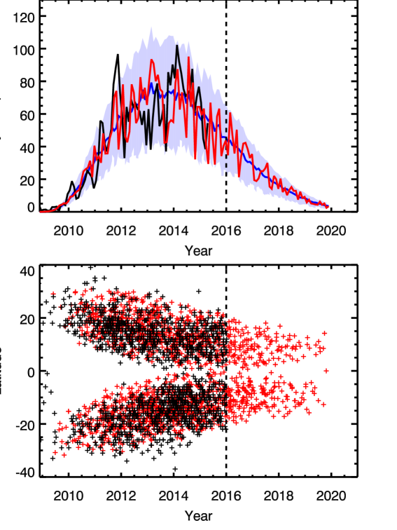
Figure 1: Example of a realization of cycle 24 with random sources. Upper panel: monthly group sunspot number (black curve: observed; red curve: one random realization; blue curve: average of 50 random realizations). The shading indicates the $\pm 2\sigma$ variation corresponding to 50 random realizations. Lower panel: butterfly diagram of emerging sunspot groups (bipolar magnetic regions). Black crosses indicate observed sunspot groups; red crosses give one realisation of random sources, corresponding to the red curve in the upper panel.

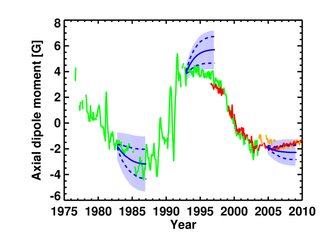
Figure 3: Evolution of the axial dipole moment for cycles 21–23. Solid blue lines show the average of 50 SFT simulations with random sources. Blue shading indicates the total $2\sigma$ uncertainty range. The dashed blue lines goive the $2\sigma$ range for the intrinsic solar contribution (source scatter). The other colored lines correspond to the values determined from the various series of synoptic magnetograms (see legend in Fig. 2).

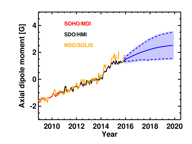
Figure 4: Predicted evolution of the axial dipole moment until 2020 (expected activity minimum of cycle 24) based on 50 SFT simulation with random sources starting from a synoptic magnetogram taken with SDO/HMI. The figure layout corresponds to that of Fig. 3. Black and orange lines indicate values determined from SDO/HMI and NSO/SOLIS data, respectively.

References

- Baumann et al. (2004) Baumann, I., Schmitt, D., Schüssler, M., & Solanki, S. K. 2004, A&A, 426, 1075
- Brandt et al. (1990) Brandt, P. N., Schmidt, W., & Steinegger, M. 1990, Sol. Phys., 129, 191
- Cameron et al. (2013) Cameron, R. H., Dasi-Espuig, M., Jiang, J., Işık, E., Schmitt, D., & Schüssler, M. 2013, A&A, 557, A141
- Cameron et al. (2010) Cameron, R. H., Jiang, J., Schmitt, D., & Schüssler, M. 2010, ApJ, 719, 264
- Cameron & Schüssler (2012) Cameron, R. H. & Schüssler, M. 2012, A&A, 548, A57
- Cameron & Schüssler (2015) —. 2015, Science, 347, 1333
- Chapman et al. (1997) Chapman, G. A., Cookson, A. M., & Dobias, J. J. 1997, ApJ, 482, 541
- Charbonneau (2010) Charbonneau, P. 2010, Living Reviews in Solar Physics, 7, 3, http://www.livingreviews.org/lrsp
- Hathaway et al. (1994) Hathaway, D. H., Wilson, R. M., & Reichmann, E. J. 1994, Sol. Phys., 151, 177
- Jiang et al. (2011) Jiang, J., Cameron, R. H., Schmitt, D., & Schüssler, M. 2011, A&A, 528, A82
- Jiang et al. (2014a) Jiang, J., Cameron, R. H., & Schüssler, M. 2014a, ApJ, 791, 5
- Jiang et al. (2015) —. 2015, ApJ, 808, L28
- Jiang et al. (2014b) Jiang, J., Hathaway, D. H., Cameron, R. H., Solanki, S. K., Gizon, L., & Upton, L. 2014b, Space Sci. Rev., 186, 491
- Leighton (1964) Leighton, R. B. 1964, ApJ, 140, 1547
- Mackay & Yeates (2012) Mackay, D. & Yeates, A. 2012, Living Reviews in Solar Physics, 9, 6
- Martin-Belda & Cameron (2016) Martin-Belda, D. & Cameron, R. H. 2016, A&A, 586, A73
- Petrovay (2010) Petrovay, K. 2010, Living Reviews in Solar Physics, 7
- Sheeley (2005) Sheeley, Jr., N. R. 2005, Living Reviews in Solar Physics, 2, 5
- Snodgrass (1983) Snodgrass, H. B. 1983, ApJ, 270, 288
- Upton & Hathaway (2014) Upton, L. & Hathaway, D. H. 2014, ApJ, 780, 5
- van Ballegooijen et al. (1998) van Ballegooijen, A. A., Cartledge, N. P., & Priest, E. R. 1998, ApJ, 501, 866
- Wang et al. (1989) Wang, Y.-M., Nash, A. G., & Sheeley, Jr., N. R. 1989, Science, 245, 712
- Wang et al. (2009) Wang, Y.-M., Robbrecht, E., & Sheeley, Jr., N. R. 2009, ApJ, 707, 1372
- Wang & Sheeley (2009) Wang, Y.-M. & Sheeley, N. R. 2009, ApJ, 694, L11