Capacity of Cellular Networks with Femtocache

Abstract

The capacity of next generation of cellular networks using femtocaches is studied when multihop communications and decentralized cache placement are considered. We show that the storage capability of future network User Terminals (UT) can be effectively used to increase the capacity in random decentralized uncoded caching. We further propose a random decentralized coded caching scheme which achieves higher capacity results than the random decentralized uncoded caching. The result shows that coded caching which is suitable for systems with limited storage capabilities can improve the capacity of cellular networks by a factor of $\log(n)$ where $n$ is the number of nodes served by the femtocache.

I Introduction

Future cellular networks require the support for high data rate video and content delivery. Many researchers have recently focused on proposing robust solutions to efficiently address the bandwidth utilization problem. For example, the authors in [5] proposed to create home sized femtocells to overcome this issue.

Golrezaei et. al [8] proposed an alternate solution by introducing the concept of femtocaching. In their solution, several helper nodes with high storage capabilites are deployed in each cell to create a distributed wireless caching infrastructure. These nodes will reduce the communication burden on the base station by satisfying many of the User Terminal (UT) requests using the stored contents in their caches. Therefore, the storage capability of helper nodes is used to increase the overall network capacity.

Currently, many researchers recommend to utilize high bandwidth Device-to-Device (D2D) and Machine-to-Machine (M2M) communication capabilities for UTs. Current IEEE 802.11ad standard [1] and the millimeter-wave proposal for future 5G networks [2, 22] are examples of such high bandwidth D2D communications which can enable up to hundreds of GHz of bandwidth. Authors in [15] suggest to use this abundant bandwidth to deliver the contents from the helper nodes to the UTs through multihop communications. Therefore, they extend the solution in [8] to allow multihop communication between the helper and the UTs. This approach can significantly reduce network deployment and maintenance costs without imposing restrictions on content delivery.

On the other hand, multihop communication between the helper node and the UTs together with the use of UTs’ storage capabilities can improve the overall network capacity. Current improvements on the storage capacity of mobile devices show that future UTs will have considerable under-utilized storage capabilities which can be effectively used to improve the network content delivery. Utilizing the storage capability of UTs allows future cellular networks to move toward a distributed D2D wireless caching network without imposing significant communication burden on the base station.

In this paper, we consider a wireless cellular network in which several helper nodes are deployed throughout the network to create a wireless distributed caching infrastructure. Each helper is serving a wireless ad hoc network of UTs through multihop communications as proposed in [15]. We assume that helpers are connected to the base station through a high bandwidth backhaul infrastructure and have access to all contents. They will use multihop communications to deliver the contents to the UTs. We assume that the UTs also use their under-utilized storage capacity to improve network content delivery. We will compute the capacity of such networks under decentralized random coded and uncoded cache placement algorithms.

In decentralized cache placement algorithms, each UT’s cache is populated independently of other UTs. In a random decentralized uncoded cache placement algorithms, contents are chosen randomly and stored in UTs cache locations. However, in a random decentralized coded cache placement algorithm, each UT stores a combination of multiple contents in its cache. The UTs will follow this process until their caches are fully populated. Coded cache placement is of interest in systems when the storage capacity of each node is limited compared to the total number of contents in the network.

This paper computes the capacity of cellular networks with multihop communications using helper and relay nodes for both uncoded and coded random decentralized cache placement algorithm. Our prior work [15] focused on multihop communications with helper nodes but without using the contents stored by the relay nodes. In this paper, the requests can be satisfied either by the helper node or a relay on the path between requesting node and the helper. As far as we know, this is the first paper to prove that coded caching which is originally motivated by the lack of sufficient storage capacity in UTs [17] can also increase the network capacity.

The rest of the paper is organized as follows. In section II, the related work is discussed and section III describes the network model considered in this paper. Section IV focuses on the capacity computation of wireless cellular networks operating under a decentralized random uncoded cache placement algorithm and section V reports the capacity for a random coded cache placement algorithm. Simulation results are reported in section VI and the paper is concluded in section VII.

II Related Work

The femtocaching network model is proposed in [8, 23] and the capacity improvement for single-hop communication is computed. In [15], the authors considered a femtocaching D2D network with multihop relaying of information from the helper to the UTs. They proposed a solution based on index coding in which the helper is utilizing the side information in the UTs to create index codes which are to be multicasted to the UTs. This way, they reduce bandwidth utilization by grouping multiple unicast transmissions into multicast transmission. However, that paper does not consider the case of coded side information and also it assumes that the relayed message from the helper cannot be changed based on the information in the relaying UTs.

Caching has been a subject of recent interest to many researchers. The fundamental limits of caching is studied in [19]. The results in [19] has been extended to include decentralized coded caching strategies in [18, 20, 9, 13]. Other researchers studied the problem of caching in wireless and D2D networks. Among them are the works of authors in [12, 11, 10]. The authors in [10] have studied the capacity of wireless D2D networks with caching in certain regimes. Our work is essentially different from all of these works in the sense that the UT always request the content from helper (femtocache) while in these papers, a wireless ad hoc network is considered where UTs’ requests can be satisfied by any of the nodes in the network. Clearly, such network model requires significant overhead to locate the nearest UT with the requested content while in our approach, the request always is sent toward the helper.

Coded caching has been previously suggested [17, 6] as an efficient caching technique for devices with small storage capacity. Our results demonstrate that apart from the practical importance of coded caching in small storage systems, it can be useful in increasing the capacity of cached networks.

III Network Model

In this paper we will study the capacity of cellular networks utilizing a distributed femtocaching infrastructure as proposed in [8]. In these networks, it is assumed that several helpers with high storage capacity are deployed throughout the network to assist the base station in delivering the contents to the UTs. The UTs can receive contents from helpers using D2D communications through either single hop [7] or multiple hops [15].

Assume that a helper is serving a D2D network of $n$ nodes. To analyze the capacity of this network, we will use the deterministic routing approach proposed in [16]. Without loss of generality, it is assumed that the UTs are distributed on a square of area one and the helper is located at the center of the square as shown in Figure 1.

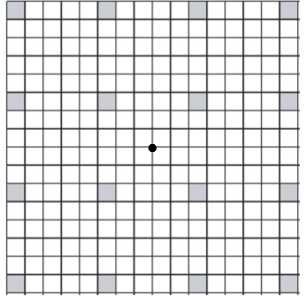
Figure 1: The helper node which is located at the center of the unit square is serving $n$ UTs which are randomly distributed on a unit square. The square is divided into $\Theta(\frac{n}{\log n})$ square-lets of area $\Theta(\frac{\log n}{n})$. Gray square-lets can transmit simultaneously. Around each grey square-lets there is a “silence” region of square-lets that are not allowed to transmit in the given time slot.

When a UT requests a content from the helper, the content is routed from the helper to the UT in a sequence of horizontal and vertical square-lets that are crossing the straight line which connects the helper to the UT. It is proved in [16] that if the UTs are uniformly distributed over the unit square area and the area is divided into $\Theta(\frac{n}{\log n})$ square-lets each with area $\Theta(\frac{\log n}{n})$, then with a probability close to one, each square-let contains $\Theta(\log n)$ UTs. A minimum transmission range of $s(n)=\Theta(\sqrt{\frac{\log n}{n}})$ ensures network connectivity [21] in such a dense network. Therefore, assuming a transmission range of $s(n)=\Theta(\sqrt{\frac{\log n}{n}})$, the proposed routing algorithm is proved to converge and all the UTs will be able to receive their requested contents with probability one.

To avoid multiple access interference, a Protocol Model is considered [24] for the successful communication between UTs. According to this model, if the UT $i$ is placed at the coordinates $Y_{i}$, then a transmission from $i$ to another UT $j$ is successful if $|Y_{i}-Y_{j}|<s(n)$ and for any other UT $k$ transmitting on the same frequency band, $|Y_{k}-Y_{j}|>(1+\Delta)s(n)$ for a fixed guard zone factor $\Delta$. A Time Division Multiple Access (TDMA) scheme is assumed for the transmission between the square-lets. With the assumption of Protocol Model, it was shown [16] that if the square-lets have a side length of $C_{1}s(n)$ for a fixed constant $C_{1}$ and if the square-lets with a distance of $C_{2}=\frac{2+\Delta}{C_{1}}$ square-lets apart from each other transmit simultaneously, then there will be no interference between the concurrent transmissions.

Lets denote the data rate for each UT by $\lambda$, the number of hops between each UT and its helper by $x$, its average value by $\mathbb{E}[x]$, and the total network throughput by $n\lambda$. Therefore, on average the network delivers $n\lambda\mathbb{E}[x]$ bits in a unit of time. There are exactly $\frac{1}{(C_{2}C_{1}s(n))^{2}}$ square-lets at any time slot available for transmission and if the total network bandwidth is $W$ which is a constant value independent of $n$, then the total number of bits that the network is capable of delivering is upper bounded [14] by $\frac{W}{(C_{2}C_{1}s(n))^{2}}$. Hence,

$$\lambda\leq\lambda_{\max}=\dfrac{W}{n\mathbb{E}[x](C_{2}C_{1}s(n))^{2}}=\Theta\left(\dfrac{1}{\mathbb{E}[x]\log n}\right).$$ (1)

This result implies that the maximum throughput can be derived by computing $\mathbb{E}[x]$. The capacity problem is therefore reduced to computing the average number of hops traveled between the UTs and the helper.

We assume the number of contents in the network is $m$ which grows polynomially with $n$ [10] as $m=C_{3}n^{\alpha}$. We denote the set of indices of all contents by $\xi=\{1,2,\dots,m\}$. Without loss of generality we assume that the contents with lower indices are more popular compared to the ones with higher indices. We further assume that the contents can be categorized into two groups of highly popular contents and less popular contents. Let’s denote the requested content by $r$, then the probability that $r$ belongs to the highly popular group of contents should be close to one. The highly popular and less popular groups can be defined as

Definition 1.

For $\epsilon\in(0,1)$, define $h_{\epsilon}$ as the smallest integer such that if $\xi_{1-\epsilon}=\{1,2,\dots,h_{\epsilon}\}$ and $\xi_{\epsilon}=\{h_{\epsilon}+1,h_{\epsilon}+2,\dots,m\}$, then $\textrm{P}[r\in\xi_{1-\epsilon}]\geq 1-\epsilon$.

We refer to $\xi_{1-\epsilon}$ as the group of highly popular contents and $\xi_{\epsilon}$ as the group of less popular contents. We assume that the helper has access to all the contents in $\xi$ but the UTs are assumed to have a limited cache of size $M=C_{4}n^{\beta}$. For the purpose of this paper, we assume that all UTs have the same cache size and the helper (or base station) is applying a decentralized caching strategy to populate a UT cache independently of other UTs. Since the UTs have limited cache size, we assume that only popular contents in $\xi_{1-\epsilon}$ are stored in UTs caches. Any request for the less popular contents from $\xi_{\epsilon}$ will be satisfied directly by the helper or base station.

When a UT $i$ requests a content, if that specific content or a group of coded contents which can be used to decode the content are available in the caches of the UTs in the routing path between the UT $i$ and the helper, then the helper informs the UTs which have the coded contents in their caches to send the content to UT $i$. If the content or a set of coded contents do not exist in the caches of the UTs between UT $i$ and helper, then the content is routed to UT $i$ from the helper through on average $s(n)^{-1}=\Theta(\sqrt{\frac{n}{\log n}})$ hops. Since majority of the requests are from popular contents, these requests can be satisfied by the UTs instead of helper which reduces the average number of transmissions per request. Therefore, provided that the content request probability distribution is known, the average number of traveled hops in the network can be written as

$$\mathbb{E}[x] = \mathbb{E}[x|r\in\xi_{\epsilon}]\textrm{P}[r\in\xi_{\epsilon}]+\mathbb{E}[x|r\in\xi_{1-\epsilon}]\textrm{P}[r\in\xi_{1-\epsilon}],$$ (2)

$$= \epsilon\sqrt{\frac{n}{\log n}}+(1-\epsilon)\mathbb{E}[x|r\in\xi_{1-\epsilon}].$$

Remark 1.

By choosing $\epsilon=\frac{1}{\sqrt{n}}$, the average hop count of the contents in $\xi_{\epsilon}$ will become less than one and therefore the total average hop count can be approximated by the average hop counts of the files in $\xi_{1-\frac{1}{\sqrt{n}}}$, i.e.,

$$\mathbb{E}[x] = \frac{1}{\sqrt{n}}\sqrt{\frac{n}{\log n}}+(1-\frac{1}{\sqrt{n}})\mathbb{E}[x|r\in\xi_{1-\frac{1}{\sqrt{n}}}]$$ (3)

$$= \Theta(\mathbb{E}[x|r\in\xi_{1-\frac{1}{\sqrt{n}}}])$$

For many web applications [3, 4], the content request popularity follows Zipfian-like distributions. Although we will express our results in general form without any specific assumption, we will later compute explicit capacity results assuming a Zipfian content popularity distribution. Our main results in proving the gain of coded caching over uncoded caching is independent of the content popularity distribution.

For a Zipfian content popularity distribution with parameter $s$, the probability of requesting a content with popularity index $i$ will have the form $\textrm{P}[r=i]=\frac{i^{-s}}{\sum_{j=1}^{m}j^{-s}}=\frac{i^{-s}}{H_{m,s}},$ where $H_{m,s}$ represents the generalized harmonic number with parameter $s$.

Remark 2.

In case of Zipfian distribution with $s>1$, when few popular contents are widely requested by the UTs, we have

$$\textrm{P}[r\in\xi_{\epsilon}]=\sum_{i=h_{\epsilon}+1}^{m}\frac{i^{-s}}{H_{m,s}}\leq\frac{(m-h_{\epsilon})(h_{\epsilon})^{-s}}{H_{m,s}}.$$ (4)

Assuming that $m=C_{3}n^{\alpha}$ is a large number, $H_{m,s}$ converges to Reimann Zeta function $\zeta(s)$. Since the number of popular contents is negligible compared to the total number of contents, $\frac{m-h_{\epsilon}}{H_{m,s}}$ can be upper bounded by $\frac{2m}{\zeta(s)}$ and therefore in case of a Zipfian distribution with $s>1$, we have

$$\textrm{P}[r\in\xi_{\epsilon}]\leq\frac{2C_{3}n^{\alpha}(h_{\epsilon})^{-s}}{\zeta(s)}.$$ (5)

In order to compute $h_{\frac{1}{\sqrt{n}}}$ such that $\textrm{P}[r\in\xi_{\frac{1}{\sqrt{n}}}]\leq\frac{1}{\sqrt{n}}$, it is sufficient to have

$$h_{\frac{1}{\sqrt{n}}}=\Theta\left(n^{\frac{1}{s}(\alpha+\frac{1}{2})}\right).$$ (6)

Since we implicitly assume that $h_{\frac{1}{\sqrt{n}}}=O(m)=O(C_{3}n^{\alpha})$, equation (6) is valid when $\alpha>\frac{1}{2(s-1)}$.

Remark 3.

In case when $\beta>\frac{1}{s}(\alpha+\frac{1}{2})$, the average number of traveled hops can be zero since in that case, all UTs can store all the popular contents in their caches. Therefore, in this case, the maximum per node capacity $\Theta(1)$ is trivially achievable.

For the rest of paper, we compute capacity assuming that the number of popular contents $h_{\epsilon}$ is known. The capacity for the special case of Zipfian distribution will be derived as well.

IV Decentralized Uncoded Caching

This section focuses on computing the capacity of cellular networks when UTs cache uncoded contents in a distributed fashion. It is assumed that the UTs only cache the most popular contents from $\xi_{1-\epsilon}$.

Lemma 1.

If a content is drawn uniformly at random from the set of most popular contents in $\xi_{1-\epsilon}$, then the average required number of requests to have at least one copy of each content from $\xi_{1-\epsilon}$ is equal to

$$\mathbb{E}[l]=h_{\epsilon}H_{h_{\epsilon}}=h_{\epsilon}\sum_{i=1}^{h_{\epsilon}}\frac{1}{i}=\Theta(h_{\epsilon}\log h_{\epsilon}),$$ (7)

where $H_{h_{\epsilon}}$ is the $h_{\epsilon}^{th}$ harmonic number. This problem is similar to the well-known coupon collector problem.

Proof.

Denote $t_{i}$ as the number of required requests to collect the $i^{th}$ content after $(i-1)^{th}$ content have been collected. Notice that the probability of collecting a new content given that $i-1$ contents have been collected is equal to $p_{i}=\frac{{h_{\epsilon}}-(i-1)}{{h_{\epsilon}}}$. Therefore, $t_{i}$ has geometric distribution with expected value of $\frac{1}{p_{i}}=\frac{{h_{\epsilon}}}{{h_{\epsilon}}-(i-1)}$. By the linearity of expectation we have:

$$\mathbb{E}[l]=\sum_{i=1}^{{h_{\epsilon}}}\mathbb{E}[t_{i}]=\sum_{i=1}^{{h_{\epsilon}}}\frac{{h_{\epsilon}}}{{h_{\epsilon}}-(i-1)}={h_{\epsilon}}\sum_{i=1}^{{h_{\epsilon}}}\frac{1}{i}=h_{\epsilon}H_{h_{\epsilon}}$$

∎

Remark 4.

Notice that the contents in UT caches should be stored such that each UT does not cache a content more than once. Therefore, this problem cannot exactly be modeled by the coupon collector problem but when $h_{\epsilon}>>M$, the probability of having multiple instances of the same content in one UT goes to zero and hence the above argument is valid and $\mathbb{E}[l]=h_{\epsilon}H_{h_{\epsilon}}$.

Note that during placement phase, we cache contents from the popular set $\xi_{1-\epsilon}$ inside the UTs independently and with uniform distribution. The distribution of placement of contents inside the UTs is different from the popularity distribution of the contents.

Theorem 1.

In a cellular network with femtocaching operating under a decentralized uncoded caching assumption, the average number of traveled hops is

$$\mathbb{E}[x]=\mathbb{E}[x|r\in\xi_{1-\frac{1}{\sqrt{n}}}]=\Theta\left(\frac{h_{\frac{1}{\sqrt{n}}}\log h_{\frac{1}{\sqrt{n}}}}{M}\right).$$ (8)

Therefore, the following capacity is achievable

$$\lambda_{\textrm{uncoded}}=\Theta(\frac{1}{\mathbb{E}[x]\log n})=\Theta\left(\frac{M}{h_{\frac{1}{\sqrt{n}}}\log h_{\frac{1}{\sqrt{n}}}\log n}\right).$$ (9)

Proof.

Lemma 1 shows that the average number of cache places needed so that all of the requests can be satisfied is $\Theta(h_{\frac{1}{\sqrt{n}}}\log h_{\frac{1}{\sqrt{n}}})$. Since each UT has a cache size $M$, it is obvious that the average number of users needed such that at least one copy of each content is available in their caches is $\Theta(\frac{h_{\frac{1}{\sqrt{n}}}\log h_{\frac{1}{\sqrt{n}}}}{M})$. Hence, along the routing path to the helper, the average number of required hops needed so that the UT can reach its desired content is $\Theta(\frac{h_{\frac{1}{\sqrt{n}}}\log h_{\frac{1}{\sqrt{n}}}}{M})$. This proves the theorem. Equation (1) can be used to compute the capacity by replacing $\mathbb{E}[x]$ with the above result. ∎

We can use equation (6) to simplify the results of theorem 9 to the case of Zipfian content request distribution.

Corollary 1.

In a cellular femtocaching network with Zipfian content request distribution with parameter $s>1$ and assuming $\alpha>\frac{1}{2(s-1)}$, the following capacity result is achievable.

$$\lambda_{\textrm{uncoded}}^{\textrm{Zipf}}=\Theta\left(n^{\beta-\frac{1}{s}(\alpha+\frac{1}{2})}\frac{1}{(\log n)^{2}}\right)$$ (10)

V Decentralized Coded Caching

In this section we will find capacity results assuming that the UTs are caching coded contents from the set of popular contents in $\xi_{1-\epsilon}$ independently of other UTs. We propose a random coding strategy and we will prove that if UTs follow this random coding strategy, the capacity will be increased by a factor of $\log h_{\epsilon}$. The result proves that not only coded caching is more efficient in small storage scenarios [17], but also it increases the capacity. We first describe the random coding cache placement and the decoding procedure.

Coded cache placement: For the purposes of this paper, we assume that random coding is done over Galois Field GF(2). For each encoded file, the helper node (or base station) randomly selects each one of contents from the set $\xi_{1-\epsilon}$ with probability $\frac{1}{2}$ and then add all the selected contents to create one encoded file. For a UT with cache size $M$, the helper node creates $M$ of these encoded files. Therefore, each one of the contents in $\xi_{1-\epsilon}$ has been used on average $\frac{M}{2}$ times to create the $M$ coded files.

Coded file reconstruction: When a UT requests a content, if the content is among the set of popular contents $\xi_{1-\epsilon}$, it sends the request to the helper. The helper then decides to send the file through a routing path as proposed in [16]. However, it is highly possible that the content can be reconstructed using the coded contents in the caches of UTs between the requesting UT and the helper along the routing path. If that is the case, then the helper sends appropriate coding information to the relaying UTs along the routing path and each relay UT that has useful information, add that information to the file that is being relayed to the requesting UT. This procedure continues hop by hop until the content reaches the requesting UT. After the requesting UT receives this file, it can reconstruct the desired content by applying its own coding gains to the received coded file. By doing so, there will not be multiple transmissions by relaying UTs to construct the requested content.

To prove our results we will first prove the following lemma.

Lemma 2.

If for a vector $v_{i}\in\mathbb{F}_{2}^{{h_{\epsilon}}}$, every element is equal to 1 with probability $\frac{1}{2}$ and equal to 0 with probability $\frac{1}{2}$ and $\{v_{1},v_{2},\dots,v_{q}\}$ span the vector space of $\mathbb{F}_{2}^{h_{\epsilon}}$, then the average required number of such vectors to span the set $\mathbb{F}_{2}^{{h_{\epsilon}}}$ equals $\mathbb{E}[q]={h_{\epsilon}}+\sum_{i=1}^{h_{\epsilon}}\frac{1}{2^{i}-1}={h_{\epsilon}}+\gamma$ where $\gamma\approx 1.6067$ is called the Erdős–Borwein constant.

Proof.

We can form a Markov chain to model the problem. The states of this Markov chain are equal to the dimension of the space spanned by vectors $v_{1},v_{2},\dots,v_{l}$. Let $k_{l}$ ($k_{l}\leq h_{\epsilon}$) denote the dimension of the space spanned by vectors $v_{1},v_{2},\dots,v_{l}$. Therefore, the Markov chain will have $k_{l}+1$ distinct states. Assuming that we are in state $k_{l}$, we want to find the probability that adding a new vector will change the state to $k_{l}+1$. When we are in state $k_{l}$, adding $2^{k_{l}}$ vectors out of the total $2^{h_{\epsilon}}$ possible vectors will not change the dimension while adding any one of $2^{h_{\epsilon}}-2^{k_{l}}$ new vectors will change the dimension to $k_{l}+1$. Therefore, the Markov chain can be represented as the one in Figure 2.

Figure 2: The state space of the Markov chain used in proof of lemma 2.

The state transition matrix for this Markov chain can be written in the form of a discrete phase-type distribution as

$$P=\begin{bmatrix}T&T_{0}\\ 0&1\\ \end{bmatrix},$$ (11)

where

$$T=\begin{bmatrix}\frac{1}{2^{h_{\epsilon}}}&1-\frac{1}{2^{h_{\epsilon}}}&0&\cdots&0&0\\ 0&\frac{2}{2^{h_{\epsilon}}}&1-\frac{2}{2^{h_{\epsilon}}}&\cdots&0&0\\ 0&0&\frac{4}{2^{h_{\epsilon}}}&\cdots&0&0\\ \vdots&\vdots&\vdots&\ddots&\vdots&\vdots\\ 0&0&0&\cdots&\frac{2^{{h_{\epsilon}}-2}}{2^{h_{\epsilon}}}&1-\frac{2^{{h_{\epsilon}}-2}}{2^{h_{\epsilon}}}\\ 0&0&0&\cdots&0&\frac{2^{{h_{\epsilon}}-1}}{2^{h_{\epsilon}}}\\ \end{bmatrix},$$ (12)

$$T_{0}^{t}=[0\hskip 7.22743pt0\ldots 1-\frac{2^{{h_{\epsilon}}-1}}{2^{h_{\epsilon}}}],$$ (13)

and $t$ denotes transpose operation. If $e$ denotes all one vector of size ${h_{\epsilon}}$, since $P$ is a probability distribution we have $P\begin{bmatrix}e\\ 1\end{bmatrix}=\begin{bmatrix}e\\ 1\end{bmatrix}.$ This implies that $Te+T_{0}=e$, hence $T_{0}=(I-T)e$. Therefore, it is easy to show by induction that the state transition matrix in $l$ steps can be written as

$$P^{l}=\begin{bmatrix}T^{l}&(I-T^{l})e\\ 0&1\\ \end{bmatrix}.$$ (14)

This equation implies that if we define the absorption time as

$$q=\inf\{l\geq 1~{}|~{}k_{l}={h_{\epsilon}}\},$$ (15)

and if $l$ is strictly less than the absorption time, the probability of transitioning from state $i$ to state $j$ by having $l$ new vectors can be found from the submatrix $T^{l}$ of $P^{l}$. In other words,

$$\mathrm{P}_{i}^{l}[k_{l}=j,l<q]=(T^{l})_{ij}.$$ (16)

Therefore, starting from state $i$, if $t_{j}^{i}$ denotes the time spent in state $j$ before absorption, $t_{j}^{i}$ can be written as

$$t_{j}^{i}=\sum_{l=0}^{q-1}\mathrm{1}\{k_{l}=j\}$$ (17)

Therefore, starting from state $i$, the average time spent in state $j$ will be equal to

$$\mathbb{E}[t_{j}^{i}]=\mathbb{E}\left[\sum_{l=0}^{q-1}\mathrm{1}\{k_{l}=j\}\right]=\sum_{l=0}^{q-1}\mathbb{E}\left[\mathrm{1}\{k_{l}=j\}\right].$$

Since $\mathbb{E}\left[\mathrm{1}\{k_{l}=j\}\right]=\mathrm{P}_{i}^{l}(k_{l}=j,l\leq q-1)$, we have

$$\mathbb{E}[t_{j}^{i}]=\sum_{l=0}^{q-1}\mathrm{P}_{i}^{l}(k_{l}=j,l\leq q-1)=\sum_{l=0}^{\infty}\mathrm{P}_{i}^{l}(k_{l}=j,l\leq q-1)$$

$$=\sum_{l=0}^{\infty}\mathrm{P}_{i}^{l}(k_{l}=j,l<q)=\sum_{l=0}^{\infty}(T^{l})_{ij}.$$ (18)

Since the probability is nonzero up to $q-1$, then we can extend the summation to infinity adding zero terms in (18). Notice that the equality in the last line comes from equation (16). If we denote matrix $U=(\mathbb{E}[t_{j}^{i}])_{ij}$, using equation (V) and using matrix algebra, we have

$$U=\sum_{i=0}^{\infty}T^{i}=(I-T)^{-1}.$$ (19)

It is not difficult to verify that

$$\\ U=(I-T)^{-1}=\begin{bmatrix}\frac{2^{h_{\epsilon}}}{2^{h_{\epsilon}}-1}&\frac{2^{{h_{\epsilon}}-1}}{2^{{h_{\epsilon}}-1}-1}&\frac{2^{{h_{\epsilon}}-2}}{2^{{h_{\epsilon}}-2}-1}&\cdots&2\\ 0&\frac{2^{{h_{\epsilon}}-1}}{2^{{h_{\epsilon}}-1}-1}&\frac{2^{{h_{\epsilon}}-2}}{2^{{h_{\epsilon}}-2}-1}&\cdots&2\\ 0&0&\frac{2^{{h_{\epsilon}}-2}}{2^{{h_{\epsilon}}-2}-1}&\cdots&2\\ \vdots&\vdots&\vdots&\ddots&\vdots\\ 0&0&0&\cdots&2\end{bmatrix}$$

Therefore, starting at $k_{l}=0$, the average time it takes to get to absorption is equal to

$$\mathbb{E}[q] = \begin{bmatrix}1&0&\cdots&0\end{bmatrix}Ue$$ (20)

$$= \begin{bmatrix}1&0&\cdots&0\end{bmatrix}(I-T)^{-1}e$$

$$= \sum_{i=1}^{h_{\epsilon}}\frac{2^{i}}{2^{i}-1}={h_{\epsilon}}+\sum_{i=1}^{h_{\epsilon}}\frac{1}{2^{i}-1}$$

This proves the lemma. ∎

This lemma shows that each UT’s request can be satisfied in a smaller number of hops compared to an uncoded caching strategy. Therefore, the capacity will be increased. The following theorem formalizes this.

Theorem 2.

In a cellular network with femtocaching, our proposed decentralized coded caching in which each popular content in $\xi_{1-\epsilon}$ is present in any cache location with probability $\frac{1}{2}$ reduces the required number of traveled hops for each request by UTs to at most

$$\mathbb{E}[x]=\mathbb{E}[x|r\in\xi_{1-\frac{1}{\sqrt{n}}}]=\Theta\left(\frac{h_{\frac{1}{\sqrt{n}}}}{M}\right).$$ (21)

Therefore, the following capacity is achievable through decentralized coded caching.

$$\lambda_{\textrm{coded}}=\Theta(\frac{1}{\mathbb{E}[x]\log n})=\Theta\left(\frac{M}{h_{\frac{1}{\sqrt{n}}}\log n}\right)$$ (22)

Proof.

Lemma 2 shows that to be able to decode a requested content, on average $\Theta(h_{\frac{1}{\sqrt{n}}})$ coded contents are required. Since each UT has a cache of size $M$, we need $\Theta(\frac{h_{\frac{1}{\sqrt{n}}}}{M})$ UTs to be able to decode the desired content. This means that along the routing path, we only need to travel a distance of $\Theta(\frac{h_{\frac{1}{\sqrt{n}}}}{M})$ hops away from each UT to find all the contents that the UT requires for decoding its desired content. Notice that individual UTs do not need to separately send their coded content to the requesting node. Each UT can combine the appropriate encoded files to the received file along the route to the requesting node. ∎

Similarly, the results of theorem 22 can be simplified by using equation (6) for the case of Zipfian content request distribution.

Corollary 2.

In a cellular femtocaching network with Zipfian content request distribution with parameter $s>1$ and assuming $\alpha>\frac{1}{2(s-1)}$, the following capacity result is achievable through decentralized coded caching.

$$\lambda_{\textrm{coded}}^{\textrm{Zipf}}=\Theta\left(n^{\beta-\frac{1}{s}(\alpha+\frac{1}{2})}\frac{1}{\log n}\right)$$ (23)

Our proposed coded caching strategy can be done with insignificant overhead as the coding instructions sent from the helper is negligible compared to the size of the files. The computational complexity of in each UT (XOR operation) is also not significant. However, the helper requires to have high computational complexity capability. Future works should concentrate on the ways to reduce the complexity and delay for this approach.

VI Simulations

The simulation results compare the performance of our proposed decentralized random coded caching with decentralized random uncoded caching. We assume a helper which is serving $n=2500$ UTs. The Zipfian content request probability parameter is $s=2.5$, $\alpha=1.5$, and $C_{3}=8$ which means that a total of $m=1000000$ contents exist in the network and 523 popular contents are considered for this simulation. The cache size parameter $\beta$ is ranging from $0.3$ to $0.8$ while $C_{4}=1$. Figure 3 shows the simulation results comparing the average number of hops required to decode the content in both decentralized coded and uncoded caching. As can be seen from this figure, our proposed decentralized random coded cache placement algorithm can significantly reduce the average number of traveled hops compared to decentralized uncoded cache placement. Further, the theoretical results match the simulation results for both cases.

Figure 3: Simulation results show that the expected number of hops in case of decentralized coded caching is significantly lower than the expected number of hops for decentralized uncoded caching.

VII Conclusions

In this paper, we studied the content delivery capacity in cellular networks with femtocaching with decentralized uncoded and coded caching for UTs. We computed the capacity of random decentralized uncoded caching. We then proposed a random coded caching strategy for network users and proved that this random coded caching technique can improve the capacity. Note that we did not consider the possibility of congestion near helper node since all contents are moving toward that node. In the future work, we intend to study the effects of congestion on the capacity of the network.

References

- [1] Amendments in IEEE 802.11ad™ enable multi-gigabit data throughput and groundbreaking improvements in capacity. https://standards.ieee.org/news/2013/802.11ad.html, 2013. [Online; accessed 9-October-2015].
- [2] Federico Boccardi, Robert W Heath, Aurelie Lozano, Thomas L Marzetta, and Petar Popovski. Five disruptive technology directions for 5G. Communications Magazine, IEEE, 52(2):74–80, 2014.
- [3] Lee Breslau, Pei Cao, Li Fan, Graham Phillips, and Scott Shenker. On the implications of Zipf’s law for web caching. Technical report, Citeseer, 1998.
- [4] Lee Breslau, Pei Cao, Li Fan, Graham Phillips, and Scott Shenker. Web caching and Zipf-like distributions: Evidence and implications. In INFOCOM’99. Eighteenth Annual Joint Conference of the IEEE Computer and Communications Societies. Proceedings. IEEE, volume 1, pages 126–134. IEEE, 1999.
- [5] Vikram Chandrasekhar, Jeffrey G Andrews, and Alan Gatherer. Femtocell networks: a survey. Communications Magazine, IEEE, 46(9):59–67, 2008.
- [6] Zhi Chen. Fundamental limits of caching: Improved bounds for small buffer users. arXiv preprint arXiv:1407.1935, 2014.
- [7] Negin Golrezaei, Andreas F Molisch, Alexandros G Dimakis, and Giuseppe Caire. Femtocaching and device-to-device collaboration: A new architecture for wireless video distribution. Communications Magazine, IEEE, 51(4):142–149, 2013.
- [8] Negin Golrezaei, Karthikeyan Shanmugam, Alexandros G Dimakis, Andreas F Molisch, and Giuseppe Caire. Femtocaching: Wireless video content delivery through distributed caching helpers. In INFOCOM, 2012 Proceedings IEEE, pages 1107–1115. IEEE, 2012.
- [9] Jad Hachem, Nikhil Karamchandani, and Suhas Diggavi. Multi-level coded caching. In Information Theory (ISIT), 2014 IEEE International Symposium on, pages 56–60. IEEE, 2014.
- [10] Sang-Woon Jeon, Song-Nam Hong, Mingyue Ji, Giuseppe Caire, and Andreas F Molisch. Wireless multihop device-to-device caching networks. arXiv preprint arXiv:1511.02574, 2015.
- [11] Mingyue Ji, Giuseppe Caire, and Andreas F Molisch. Wireless device-to-device caching networks: Basic principles and system performance. arXiv preprint arXiv:1305.5216, 2013.
- [12] Mingyue Ji, Giuseppe Caire, and Andreas F Molisch. Fundamental limits of caching in wireless D2D networks. arXiv preprint arXiv:1405.5336, 2014.
- [13] Nikhil Karamchandani, Urs Niesen, Mohammad Ali Maddah-Ali, and Suhas Diggavi. Hierarchical coded caching. In Information Theory (ISIT), 2014 IEEE International Symposium on, pages 2142–2146. IEEE, 2014.
- [14] Mohsen Karimzadeh Kiskani, Bita Azimdoost, and Hamid Sadjadpour. Effect of social groups on the capacity of wireless networks. Wireless Communications, IEEE Transactions on, 2015.
- [15] Mohsen Karimzadeh Kiskani and Hamid R. Sadjadpour. Multihop caching-aided coded multicasting for the next generation of cellular networks. arXiv preprint arXiv:1412.2391, 2015.
- [16] Sanjeev R Kulkarni and Pramod Viswanath. A deterministic approach to throughput scaling in wireless networks. Information Theory, IEEE Transactions on, 50(6):1041–1049, 2004.
- [17] Namyoon Lee, Alexandros G Dimakis, and Robert W Heath. Index coding with coded side-information. Communications Letters, IEEE, 19(3):319–322, 2015.
- [18] Mohammad Ali Maddah-Ali and Urs Niesen. Decentralized coded caching attains order-optimal memory-rate tradeoff. In Communication, Control, and Computing (Allerton), 2013 51st Annual Allerton Conference on, pages 421–427. IEEE, 2013.
- [19] Mohammad Ali Maddah-Ali and Urs Niesen. Fundamental limits of caching. Information Theory, IEEE Transactions on, 60(5):2856–2867, 2014.
- [20] Ramtin Pedarsani, Mohammad Ali Maddah-Ali, and Urs Niesen. Online coded caching. In Communications (ICC), 2014 IEEE International Conference on, pages 1878–1883. IEEE, 2014.
- [21] Mathew D Penrose. The longest edge of the random minimal spanning tree. The annals of applied probability, pages 340–361, 1997.
- [22] Theodore S Rappaport, Shu Sun, Rimma Mayzus, Hang Zhao, Yaniv Azar, Kangping Wang, George N Wong, Jocelyn K Schulz, Mathew Samimi, and Felix Gutierrez. Millimeter wave mobile communications for 5G cellular: It will work! Access, IEEE, 1:335–349, 2013.
- [23] Karthikeyan Shanmugam, Negin Golrezaei, Alexandros G Dimakis, Andreas F Molisch, and Giuseppe Caire. Femtocaching: Wireless content delivery through distributed caching helpers. Information Theory, IEEE Transactions on, 59(12):8402–8413, 2013.
- [24] Feng Xue and Panganamala R Kumar. Scaling laws for ad hoc wireless networks: an information theoretic approach. Now Publishers Inc, 2006.