Chained Gaussian Processes

Abstract

Gaussian process models are flexible, Bayesian non-parametric approaches to regression. Properties of multivariate Gaussians mean that they can be combined linearly in the manner of additive models and via a link function (like in generalized linear models) to handle non-Gaussian data. However, the link function formalism is restrictive, link functions are always invertible and must convert a parameter of interest to a linear combination of the underlying processes. There are many likelihoods and models where a non-linear combination is more appropriate. We term these more general models Chained Gaussian Processes: the transformation of the GPs to the likelihood parameters will not generally be invertible, and that implies that linearisation would only be possible with multiple (localized) links, i.e. a chain. We develop an approximate inference procedure for Chained GPs that is scalable and applicable to any factorized likelihood. We demonstrate the approximation on a range of likelihood functions.

1 Introduction

Gaussian process models are flexible distributions that can provide priors over non linear functions. They rely on properties of the multivariate Gaussian for their tractability and their non-parametric nature. In particular, the sum of two functions, drawn from a Gaussian process is also given by a Gaussian process. Mathematically, if $f\sim\mathcal{N}\left(\mu_{f},k_{f}\right)$ and $g\sim\mathcal{N}\left(\mu_{g},k_{f}\right)$ and we define $y=g+f$ then properties of multivariate Gaussian give us that $y\sim\mathcal{N}\left(\mu_{f}+\mu_{g},k_{f}+k_{g}\right)$ where $\mu_{f}$ and $\mu_{g}$ are deterministic functions of a single input, $k_{f}$ and $k_{g}$ are deterministic, positive semi definite functions of two inputs and $y$, $g$ and $f$ are stochastic processes.

This elementary property of the Gaussian process is the foundation of much of its power. It makes additive models trivial, and means we can easily combine any process with Gaussian noise. Naturally, it can be applied recursively, and covariance functions can be designed to reflect the underlying structure of the problem at hand (e.g. Hensman et al. (2013b) uses additive structure to account for variation in replicate behavior in gene expression).

In practice observations are often non Gaussian. In response, statistics has developed the field of generalized linear models (Nelder and Wedderburn, 1972). In a generalized linear model a link function is used to connect the mean function of the Gaussian process with the mean function of another distribution of interest. For example, the log link can be used to relate the rate in a Poisson distribution with our GP, $\log\lambda=f+g$. Or for classification the logistic distribution can be used to represent the mean probability of positive outcome, $\log\frac{p}{1-p}=f+g$.

Writing models in terms of the link function captures the linear nature of the underlying model, but it is somewhat against the probabilistic approach to modeling where we consider the generative model of our data. While there’s nothing wrong with this relationship mathematically, when we consider the generative model we never apply the link function directly, we consider the inverse link or transformation function. For the log link this turns into the exponential, $\lambda=\exp(f+g)$. Writing the model in this form emphasizes the importance that the transformation function has on the generative model (see e.g. work on warped GPs (Snelson et al., 2004)). The log link implies a multiplicative combination of $f$ and $g$, $\lambda=\exp(f+g)=\exp(f)\exp(g)$, but in some cases we might wish to consider an additive model, $\lambda=\exp(f)+\exp(g)$. Such a model no longer falls within the class of generalized linear models as there is no link function that renders the two underlying processes additive Gaussian. In this paper we address this issue and use variational approximations to develop a framework for non-linear combination of the latent processes. Because these models cannot be written in the form a single link function we call this approach “Chained Gaussian Processes”.

In this paper we are interested in performing variational inference when we have input-dependent likelihood parameters. We will focus on the case when where the likelihood contains two latent parameters, though the model is general enough to handle more. Parameters of interest could be a latent mean which we wish to infer, a shape parameter for determining the shape of the tails, amongst other things. We will focus on the cases where we have two such latent parameters but propose methods for extending this further.

We will focus on likelihoods $p(\mathbf{y}|{\bf f},{\bf g})$ that depend on two latent functions, ${\bf f}\sim\mathcal{N}\left({\bf f}|{\bm{\mu}}_{f},f(\mathbf{x})\right)$, ${\bf g}\sim\mathcal{N}\left({\bf g}|{\bm{\mu}}_{g},g(\mathbf{x})\right)$. If this noise distribution is a Gaussian then we have two special cases, with $g(\mathbf{x})=\sigma^{2}$ we have a Gaussian process with the conjugate homogeneous Gaussian likelihood. With $g(\mathbf{x})=e^{g(\mathbf{x})}$ we obtain a model for a heteroscedastic Gaussian process (Lazaro-Gredilla and Titsias, 2011).

A range of other noise models require multiple parameters to be learnt. Traditionally within the Gaussian process literature MAP solutions are used, or alternatively these parameters are integrated out approximately (Rue et al., 2009). In this work we accept that these parameters may change as a function of the input space, and look at inferring posterior Gaussian process functions for these parameters. We do so in a scalable way with sparse variational methods, with the capability of using stochastic gradients during inference. We believe scalability is essential as parameters may only become well determined as the number of observations grow large. We show results with a number of different noise models

We will first introduce notation, and review previous work on heteroscedastic Gaussian processes. Then, we show how to elegantly extend this idea into a more scalable and general framework, allowing a huge number of likelihoods to utilise multiple input dependent processes.

2 Background

Assume we have access to a training dataset of $n$ input-output observations $\{(\mathbf{x}_{i},y_{i})\}^{n}_{i=1}$, $y_{i}$ is assumed to be a noisy realisation of an underlying latent function ${\bf f}=f(\mathbf{x})$, i.e. $y_{i}=f(\mathbf{x}_{i})+\epsilon_{i}$. For a Gaussian likelihood $\epsilon_{i}\sim\mathcal{N}\left(\mu,\sigma^{2}\right)$, $\mathbf{x}_{i}\in\mathbb{R}^{q}$ and $y_{i}\in\mathbb{R}$. Normally the mean of the likelihood is assumed to be input dependent and given a GP prior $\mu={\bf f}_{i}=f(\mathbf{x}_{i})$ where $f(\mathbf{x})\sim\mathcal{GP}({\bm{\mu}}_{f},k_{g}(\mathbf{x},\mathbf{x}^{\prime}))$, and $\sigma$ is fixed at an optimal point. In this case the integrals required to infer a posterior, $p({\bf f}|\mathbf{y})$, are tractable.

One extension of this model is the heteroscedastic GP regression model (Goldberg et al., 1998; Lazaro-Gredilla and Titsias, 2011), where the noise variance $\sigma$ is dependent on the input. The noise variance can be assigned a log GP prior, $y_{i}\sim\mathcal{N}\left(f(\mathbf{x}_{i}),e^{g(\mathbf{x}_{i})}\right)$, where $g(\mathbf{x})=\mathcal{GP}({\bm{\mu}}_{g},k_{g}(\mathbf{x},\mathbf{x}^{\prime}))$, i.e. a log link function is used. Unfortunately this generalization of the original Gaussian process model is not analytically tractable and requires an approximation to be made. Suggested approximations include MCMC (Goldberg et al., 1998), variational inference (Lazaro-Gredilla and Titsias, 2011), Laplace approximation (Vanhatalo et al., 2013) and expectation propagation (Hernández-Lobato et al., 2014) (EP).

Another generalization of the standard GP is to vary the scale of the process as a function of the inputs. Adams and Stegle (2008) suggest a log GP prior for the scale of the process giving rise to non-parametric non-stationarity in the model. Turner and Sahani (2011) took a related approach to develop probabilistic amplitude demodulation, here the amplitude (or scale) of the process was given by a Gaussian process with a link function given by $\sigma=\log(\exp(f)-1)$. Finally Tolvanen et al. (2014) assign both the noise variance and the scale a log GP prior.

Both these two variations on Gaussian process regression combine processes in a non-linear way within a Gaussian likelihood, but the idea may be further generalized to systems that deal with non-Gaussian observation noise.

In this paper we describe a general approach to combining processes in a non-linear way. We assume that the likelihood factorizes across the data, but is a general non-linear function of $b$ input dependent latent functions. Our main focus will be examples of likelihoods with $b=2$, $f(\mathbf{x}_{i})$ and $g(\mathbf{x}_{i})$, such that, $p(\mathbf{y}|f(\mathbf{x}_{i}),g(\mathbf{x}_{i}))$, though the ideas can all be generalized to $b>2$. Previous work in this domain include the use of the Laplace approximation (Vanhatalo et al., 2013), however this method scales poorly, $\mathcal{O}(b^{3}n^{3})$ and so isn’t applicable to datasets of a moderate size.

To render the model tractable we extend recent advances in large scale variational inference approaches to GPs (Hensman et al., 2013a). With non-Gaussian likelihoods restrictions on the latent function values may differ, and a non-linear transformation of the latent function, ${\bf g}\in\mathbb{R}^{q}$ may be required. The inference approach builds on work by Hensman et al. (2015), that in turn builds on the variational inference method proposed by Opper and Archambeau (2009).

In other work (Nguyen and Bonilla, 2014) mixtures of Gaussian latent functions have also been applied for non-Gaussian likelihoods, we expect such mixture distributions would also be applicable to our case. More recently this approach (Dezfouli and Bonilla, 2015) was extended to provide scalability utilising sparse methods similar to this work.

3 Chained Gaussian Processes

Our approach to approximate inference in chained GPs builds on previous work in inducing point methods for sparse approximations of GPs (Snelson and Ghahramani, 2006; Titsias, 2009; Hensman et al., 2015, 2013a). Inducing point methods introduce $m$ ‘pseudo inputs’, known as inducing inputs, at locations $\mathbf{{Z}}=\{\mathbf{z}_{i}\}^{m}_{i=1}$. The corresponding function values are given by ${\bf u}_{i}=f(\mathbf{z}_{i})$. These inducing inputs points do not effect the marginal of ${\bf f}$ because

$$p({\bf f}|\mathbf{{X}},\mathbf{{Z}})=\int p({\bf f}|{\bf u},\mathbf{{X}})p({\bf u}|\mathbf{{Z}})d{\bf u},$$

where $p({\bf u}|\mathbf{{Z}})=\mathcal{N}\left({\bf u}|0,\mathbf{{K}}_{\mathbf{u}\mathbf{u}}\right)$ and $p({\bf f}|{\bf u},\mathbf{{X}})=\mathcal{N}\left({\bf f}|\mathbf{{K}}_{\mathbf{f}\mathbf{u}}\mathbf{{K}}_{\mathbf{u}\mathbf{u}}^{-1}{\bf u},\mathbf{{K}}_{\mathbf{f}\mathbf{f}}-\mathbf{{K}}_{\mathbf{f}\mathbf{u}}\mathbf{{K}}_{\mathbf{u}\mathbf{u}}^{-1}\mathbf{{K}}_{\mathbf{u}\mathbf{f}}\right)$. The part-covariances given by $\mathbf{{K}}_{\mathbf{f}\mathbf{u}}=k_{f}(\mathbf{{X}},\mathbf{{Z}})$ where $\mathbf{{X}}$ is the locations of ${\bf f}$, define the relationship between inducing variables and the latent function of interest, $f$. The marginal likelihood is $p(\mathbf{y})=\int p(\mathbf{y}|{\bf f})p({\bf f}|{\bf u})p({\bf u})d{\bf f}\,d{\bf u}$. To avoid $\mathcal{O}(n^{3})$ computation complexity Titsias (2009) invokes Jensen’s inequality to obtain a lower bound on the marginal likelihood $\log p(\mathbf{y})$, an approach known as variational compression. This approximation also forms the basis of our approach for non-Gaussian models.

3.1 Variational Bound

For non-Gaussian likelihoods, even with a single latent process the marginal likelihood, $p(\mathbf{y})$, is not tractable, but it can be lower bounded variationally. We assume that the latent functions, ${\bf f}=f(\mathbf{x})$ and ${\bf g}=g(\mathbf{x})$ are a priori independent

$$p({\bf f},{\bf g}|{\bf u}_{f},{\bf u}_{g})=p({\bf f}|{\bf u}_{f})p({\bf g}|{\bf u}_{g}).$$ (1)

The derivation of the variational lower bound then follows a similar form as (Hensman et al., 2015) with the extension to multiple latent functions. We begin by writing down our log marginal likelihood,

$$\log p(\mathbf{y}) =\log\int p(\mathbf{y}|{\bf f},{\bf g})p({\bf f},{\bf g}|{\bf u}_{f},{\bf u}_{g})p({\bf u}_{f})p({\bf u}_{g})d{\bf f}\,d{\bf g}\,d{\bf u}_{f}\,d{\bf u}_{g}$$

then introduce a variational approximation to the posterior,

$$p({\bf f},{\bf g},{\bf u}_{g},{\bf u}_{f}|\mathbf{y})\approx p({\bf f}|{\bf u}_{f})p({\bf g}|{\bf u}_{g})q({\bf u}_{f})q({\bf u}_{g}),$$ (2)

where we have made the additional assumption that the latent functions factorize in the variational posterior.

Using Jensen’s inequality and the factorization of the latent functions (1), a variational lower bound can then be obtained for the log marginal likelihood,

$$\log p(\mathbf{y}) =\log\int p(\mathbf{y}|{\bf f},{\bf g})p({\bf f}|{\bf u}_{f})p({\bf g}|{\bf u}_{g})p({\bf u}_{f})p({\bf u}_{g})d{\bf f}\,d{\bf g}\,d{\bf u}_{f}\,d{\bf u}_{g}$$

$$\geq\int q({\bf f})q({\bf g})\log p(\mathbf{y}|{\bf f},{\bf g})d{\bf f}\,d{\bf g}-\text{KL}\left(q({\bf u}_{f})\,\|\,p({\bf u}_{f})\right)-\text{KL}\left(q({\bf u}_{g})\,\|\,p({\bf u}_{g})\right),$$ (3)

where $q({\bf f})=\int p({\bf f}|{\bf u}_{f})q({\bf u}_{f})d{\bf u}_{f}$ and $q({\bf g})=\int p({\bf g}|{\bf u}_{g})q({\bf u}_{g})d{\bf u}_{g}$, and $\text{KL}\left(p(a)\,\|\,p(b)\right)$ denotes the KL divergence between the two distributions. For Gaussian process priors on the latent functions we recover

$$p({\bf f}|{\bf u}_{f}) =\mathcal{N}\left({\bf f}|\mathbf{{K}}_{{\bf f}{\bf u}_{f}}\mathbf{{K}}_{{\bf u}_{f}{\bf u}_{f}}^{-1}{\bf u}_{f},\mathbf{{K}}_{{\bf f}{\bf f}}-{\bf Q}_{\mathbf{f}\mathbf{f}}\right)$$

$$p({\bf g}|{\bf u}_{g}) =\mathcal{N}\left({\bf g}|\mathbf{{K}}_{{\bf g}{\bf u}_{g}}\mathbf{{K}}_{{\bf u}_{g}{\bf u}_{g}}^{-1}{\bf u}_{g},\mathbf{{K}}_{{\bf g}{\bf g}}-\mathbf{Q}_{{\bf g}{\bf g}}\right),$$

where

$${\bf Q}_{\mathbf{f}\mathbf{f}}=\mathbf{{K}}_{{\bf f}{\bf u}_{f}}\mathbf{{K}}_{{\bf u}_{f}{\bf u}_{f}}^{-1}\mathbf{{K}}_{{\bf u}_{f}{\bf f}}$$

$$\mathbf{Q}_{{\bf g}{\bf g}}=\mathbf{{K}}_{{\bf g}{\bf u}_{g}}\mathbf{{K}}_{{\bf u}_{g}{\bf u}_{g}}^{-1}\mathbf{{K}}_{{\bf u}_{g}{\bf g}}.$$

Note that covariances for ${\bf f}$ and ${\bf g}$, can differ though their inducing input locations, $\mathbf{{Z}}$, are shared.

We take $q({\bf u}_{f})$ and $q({\bf u}_{g})$ to be Gaussian distributions with variational parameters, ${q({\bf u}_{f})=\mathcal{N}\left({\bf u}_{f}|{\bm{\mu}}_{f},{\bm{S}}_{f}\right)}$ and ${q({\bf u}_{g})=\mathcal{N}\left({\bf u}_{g}|{\bm{\mu}}_{g},{\bm{S}}_{g}\right)}$. Using the properties of multivariate Gaussians this results in tractable integrals for $q({\bf f})$ and $q({\bf g})$,

$$q({\bf f}) =\mathcal{N}\left({\bf f}|\mathbf{{K}}_{{\bf f}{\bf u}_{f}}\mathbf{{K}}_{{\bf u}_{f}{\bf u}_{f}}^{-1}{\bm{\mu}}_{f},\mathbf{{K}}_{{\bf f}{\bf f}}+\mathbf{\hat{Q}}_{{\bf f}{\bf f}}\right)$$ (4)

$$q({\bf g}) =\mathcal{N}\left({\bf g}|\mathbf{{K}}_{{\bf g}{\bf u}_{g}}\mathbf{{K}}_{{\bf u}_{g}{\bf u}_{g}}^{-1}{\bm{\mu}}_{g},\mathbf{{K}}_{{\bf g}{\bf g}}+\mathbf{\hat{Q}}_{{\bf g}{\bf g}}\right),$$ (5)

where

$$\mathbf{\hat{Q}}_{{\bf f}{\bf f}}=\mathbf{{K}}_{{\bf f}{\bf u}_{f}}\mathbf{{K}}_{{\bf u}_{f}{\bf u}_{f}}^{-1}({\bm{S}}_{f}-\mathbf{{K}}_{{\bf u}_{f}{\bf u}_{f}})\mathbf{{K}}_{{\bf u}_{f}{\bf u}_{f}}^{-1}\mathbf{{K}}_{{\bf u}_{f}{\bf f}}$$

$$\mathbf{\hat{Q}}_{{\bf g}{\bf g}}=\mathbf{{K}}_{{\bf g}{\bf u}_{g}}\mathbf{{K}}_{{\bf u}_{g}{\bf u}_{g}}^{-1}({\bm{S}}_{g}-\mathbf{{K}}_{{\bf u}_{g}{\bf u}_{g}})\mathbf{{K}}_{{\bf u}_{g}{\bf u}_{g}}^{-1}\mathbf{{K}}_{{\bf u}_{g}{\bf g}}.$$

The KL terms in (3) and their derivative can be computed in closed form and are inexpensive as they are divergence between Gaussians. However, an intractable integral, ${\int q({\bf f})q({\bf g})\log p(\mathbf{y}|{\bf f},{\bf g})d{\bf f}\,d{\bf g}}$, still remains. Since the likelihood factorizes,

$$p(\mathbf{y}|{\bf f},{\bf g})=\prod\nolimits^{n}_{i=1}p(\mathbf{y}_{i}|{\bf f}_{i},{\bf g}_{i}),$$

the problematic integral in (3) also factorizes across data points, allowing us to use stochastic variational inference (Hensman et al., 2013a; Hoffman et al., 2013),

$$\int q({\bf f})q({\bf g})\log p(\mathbf{y}|{\bf f},{\bf g})d{\bf f}\,d{\bf g} =\int q({\bf f})q({\bf g})\log\prod^{n}_{i=1}p(\mathbf{y}_{i}|{\bf f}_{i},{\bf g}_{i})d{\bf f}\,d{\bf g}$$

$$=\sum\nolimits^{n}_{i=1}\int q({\bf f}_{i})q({\bf g}_{i})\log p(\mathbf{y}_{i}|{\bf f}_{i},{\bf g}_{i})d{\bf f}_{i}\,d{\bf g}_{i}.$$ (6)

We are then left with $n$, $b$ dimensional Gaussian integrals over the log-likelihood,

$$\log p(\mathbf{y}) \geq\sum\nolimits^{n}_{i=1}\int q({\bf f}_{i})q({\bf g}_{i})\log p(\mathbf{y}_{i}|{\bf f}_{i},{\bf g}_{i})d{\bf f}_{i}\,d{\bf g}_{i}$$

$$\quad-\text{KL}\left(q({\bf u}_{f})\,\|\,p({\bf u}_{f})\right)-\text{KL}\left(q({\bf u}_{g})\,\|\,p({\bf u}_{g})\right).$$ (7)

The bound will also hold for any additional number of latent functions by assuming they all factorize in the variational posterior.

The bound decomposes into a sum over data, as such the $n$ input points can be visited in mini-batches, and the gradients and log-likelihood of each mini-batch can be subsequently summed, this operation can be also be parallelized (Gal et al., 2014). A single mini-batch can instead be visited obtaining a stochastic gradient for use in a stochastic optimization (Hensman et al., 2013a; Hoffman et al., 2013). This provides the ability to scale to huge datasets.

If the likelihood is Gaussian these integrals are analytic (Lazaro-Gredilla and Titsias, 2011), though the noise variance must be constrained positive via a transformation of the latent function, e.g an exponent. In this case,

$$\int q({\bf f}_{i})q({\bf g}_{i})\log p(\mathbf{y}_{i}|{\bf f}_{i},{\bf g}_{i})d{\bf f}_{i}\,d{\bf g}_{i}$$

$$\quad=\int\mathcal{N}\left({\bf f}_{i}|{{\bm{m}}_{f}}_{i},{{\bm{v}}_{f}}_{i}\right)\mathcal{N}\left({\bf g}_{i}|{{\bm{m}}_{g}}_{i},{{\bm{v}}_{g}}_{i}\right)\log\mathcal{N}\left(\mathbf{y}_{i}|{\bf f}_{i},e^{{\bf g}_{i}}\right)$$

$$\quad=\log\mathcal{N}\left(\mathbf{y}_{i}|{{\bm{m}}_{f}}_{i},e^{{{\bm{m}}_{g}}_{i}-\frac{{{\bm{v}}_{g}}_{i}}{2}}\right)-\frac{{{\bm{v}}_{g}}_{i}}{4}-\frac{{{\bm{v}}_{f}}_{i}e^{-{{\bm{m}}_{g}}_{i}+\frac{{{\bm{v}}_{g}}_{i}}{2}}}{2}$$

where we define

$${{\bm{m}}_{f}}=\mathbf{{K}}_{{\bf f}{\bf u}_{f}}\mathbf{{K}}_{{\bf u}_{f}{\bf u}_{f}}^{-1}{\bm{\mu}}_{f} {{\bm{v}}_{f}}=\mathbf{{K}}_{{\bf f}{\bf f}}+\mathbf{\hat{Q}}_{{\bf f}{\bf f}}$$

$${{\bm{m}}_{g}}=\mathbf{{K}}_{{\bf g}{\bf u}_{g}}\mathbf{{K}}_{{\bf u}_{g}{\bf u}_{g}}^{-1}{\bm{\mu}}_{g} {{\bm{v}}_{g}}=\mathbf{{K}}_{{\bf g}{\bf g}}+\mathbf{\hat{Q}}_{{\bf g}{\bf g}}.$$

${{\bm{v}}_{f}}_{i}$ denotes the $i$th diagonal element of the matrix with ${{\bm{v}}_{f}}$ along its diagonal. It may be possible in this Gaussian case to find the optimal $q({\bf f})$ such that the bound collapses to that of Lazaro-Gredilla and Titsias (2011), however this would not allow for stochastic optimization. Here we arrive at a sparse extension, where a Gaussian distribution is assumed for the posterior over of ${\bf f}$, where as previously $q({\bf f})$ has been collapsed out and could take any form. This sparse extension provides the ability to scale to much larger datasets whilst maintaining a similar variational lower bound.

The model is however not restricted to heteroscedastic Gaussian likelihoods. If the integral (6) and its gradients can be computed in an unbiased way, any factorizing likelihood can be used. This can be seen as a chained Gaussian process. There is no single link function that allows the specification of this model under the modelling assumptions of a generalised linear model. An example that will be revisited in the experiments is the beta distribution, $y_{i}\sim B(\alpha,\beta)$ where $\alpha,\beta\in\mathbb{R}^{+}$ and observations $y_{i}\in(0,1)$, $\mathbf{x}_{i}\in\mathbb{R}^{q}$. Since $\alpha,\beta$ must maintain positiveness, then can be assigned log GP priors,

$$y_{i}\sim B(\alpha=e^{f(\mathbf{x}_{i})},\beta=e^{g(\mathbf{x}_{i})}),$$ (8)

where $f(\mathbf{x})=\mathcal{GP}({\bm{\mu}}_{f},k_{f}(\mathbf{x},\mathbf{x}^{\prime}))$ and $g(\mathbf{x})=\mathcal{GP}({\bm{\mu}}_{g},k_{g}(\mathbf{x},\mathbf{x}^{\prime}))$. This allows the shape of the beta distribution to change over time, see Supplementary Material and section 4.2.2 for an example plots.

Using the variational bound above, all that is required is to perform a series of $n$ two dimensional quadratures, for both the log-likelihood and its gradients, a relatively simple task and computationally feasible when looking at modest batch sizes. From this example the power and adaptability of the method should be apparent.

A major strength of this method is that performing this integral is the only requirement to implement a new noise model, similarly to (Nguyen and Bonilla, 2014; Hensman et al., 2015). Further, since a stochastic optimizer is used the gradients do not need to be exact. Our implementations can use off the shelf stochastic optimizer, such as Adagrad (Duchi et al., 2011) or RMSProp (Tieleman and Hinton, 2012). Further, for many likelihoods some portion of these integrals is analytically tractable, reducing the variance introduced by numerical integration. See supplementary material for an investigation.

3.2 Posterior and Predictive Distributions

Following from (2) it is clear that when the variational lower bound bound has been maximised with respect to the variational parameters, $p({\bf u}_{f}|\mathbf{y})\approx q({\bf u}_{f})$ and $p({\bf u}_{g}|\mathbf{y})\approx q({\bf u}_{g})$. The posterior for $p({\bf f}^{*}|\mathbf{y}^{*})$ under this approximation is

$$p({\bf f}^{*}|\mathbf{y}^{*}) =\int p({\bf f}^{*}|\mathbf{x},{\bf f})p({\bf f}|{\bf u}_{f})p({\bf u}_{f}|\mathbf{y})d{\bf f}\,d{\bf u}_{f}$$

$$=\int p({\bf f}^{*}|{\bf u}_{f})p({\bf u}_{f}|\mathbf{y})d{\bf u}_{f}$$

$$\approx\int p({\bf f}^{*}|{\bf u}_{f})q({\bf u}_{f})d{\bf u}_{f}=q({\bf f}^{*}),$$

where $q({\bf f}^{*})$ and $q({\bf g}^{*})$ become similar to (4).

Finally, treating each prediction point independently, the predictive distribution for each data pair $\{(\mathbf{x}_{i}^{*},\mathbf{y}^{*}_{i})\}^{n^{*}}_{i=1}$ follows as

$$p(\mathbf{y}_{i}^{*}|\mathbf{y}_{i},\mathbf{x}_{i}) =\int p(\mathbf{y}_{i}^{*}|{\bf f}_{i}^{*},{\bf g}_{i}^{*})q({\bf f}_{i}^{*})q({\bf g}_{i}^{*})d{\bf f}_{i}^{*}\,d{\bf g}_{i}^{*}.$$

This integral is analytically intractable in the general case, but again can be computed using a series of two dimensional quadrature or simple Monte Carlo sampling.

4 Experiments

To evaluate the effectiveness of our chained GP approximations we consider a range of real and synthetic datasets. The performance measure used throughout is the negative log predictive density (NLPD) on held out data, table 1. The results for mean absolute error (MAE) (Supplementary Material) show comparable results between methods. 5-fold cross-validation is used throughout. The non-linear optimization of (hyper-) parameters is subject to local minima, as such multiple runs were performed on each fold with a range of parameter initialisations. The solution obtaining the highest log-likelihood on the training data of each fold was retained. Automatic relevance determination exponentiated quadratic kernels are used throughout allowing one lengthscale per input dimension, in addition to a bias kernel... In all experiments 100 inducing points were used and their locations were optimized with respect to the lower bound of the log marginal likelihood following (Titsias, 2009).

Data	NLPD
	G	CHG	Lt	Vt	CHt
elevators1000	$0.39\pm 0.13$	$0.1\pm 0.01$	NA	NA	NA
elevators10000	$0.07\pm 0.01$	$0.03\pm 0.02$	NA	NA	NA
motorCorrupt	$2.04\pm 0.06$	$1.79\pm 0.05$	$1.73\pm 0.05$	$2.52\pm 0.09$	$1.7\pm 0.05$
boston	$0.27\pm 0.02$	$0.09\pm 0.01$	$0.23\pm 0.02$	$0.19\pm 0.02$	$0.09\pm 0.02$

Table 1: Results NLPD over 5 cross-validation folds with 10 replicates each. Models shown in comparison are sparse Gaussian (G), chained heteroscedastic Gaussian (CHG), Student-$t$ Laplace approximation (Lt), Student-$t$ VB approximation (Vt), and chained heteroscedastic Student-$t$ (CHt).

4.1 Heteroscedastic Gaussian

In our introduction we related our ideas to heteroscedastic GPs. We will first use our approximations to show how the addition of input dependent noise to a Gaussian process regression model effects performance, compared with a sparse Gaussian process model (Titsias, 2009). Performance is shown to improve as more data is provided as would be expected, making it clear that both models can scale with data, though the new model is more flexible when handling the distributions tails. A sparse Gaussian process with Gaussian likelihood is chosen in these experiments as a baseline, as a non-sparse Gaussian process cannot scale to the size of all the experiments.

The Elevator1000 uses a subset of $1,000$ of the Elevator dataset . In this data the heteroscedastic model (Chained GP) offers considerable improvement in terms of negative log predictive density (NLPD) over the sparse GP (Table 1. Our second experiment with the Gaussian likelihood, Elevator10000, examines scaling of the model. Here a subset of $10,000$ data points of the Elevator dataset are used, and performance is improved as expected. Previous models for heteroscedastic Gaussian process models cannot scale, the chained GP can implement the heteroscedastic setting and scale.

(a) NLPD motor

(b) NLPD Boston

Figure 1: 1) NLPD on corrupt motorcycle dataset. 1) NLPD of Boston housing dataset. In NLPD lower is better, models shown in comparison are sparse Gaussian (G), Student-$t$ Laplace approximation (Lt), Student-$t$ VB approximation (Vt), chained heteroscedastic Gaussian (CHG), and chained heteroscedastic Student-$t$ (CHt). Boxplots show the variation over 5 folds.

4.2 Non-Gaussian Heteroscedastic likelihoods

One of the major strengths of the approximation over pure scalability, is the ability to use more general non-Gaussian likelihoods. In this section we will investigate this flexibility by performing inference with non-standard likelihoods. This allows models to be specified that correspond to the modellers belief about the data in a flexible way.

We first investigate an extension of the Student-$t$ likelihood that endows it with an input-dependent scale parameter. This is straightforward in the chained GP paradigm.

The corrupt motorcycle dataset is an artificial modification to the benchmark motorcycle dataset (Silverman, 1985) and shows the models capabilities more clearly. The original motorcycle dataset has had 25 of its data randomly corrupted with Gaussian noise of $\mathcal{N}\left(0,3\right)$, simulating spurious accelerometer readings. We hope that our method will be robust and ignore such outlying values. An input-dependent mean, $\mu$, is set alongside an input dependent scale which must be positive, $\sigma$. A constant degrees of freedom parameter $\nu$, is initalized to 4.0 and then is optimized to its MAP solution.

$$y_{i}\sim St(\mu=f(\mathbf{x}_{i}),\sigma^{2}=e^{g(\mathbf{x}_{i})},\nu)$$ (9)

where $f(\mathbf{x})=\mathcal{GP}({\bm{\mu}}_{f},k_{f}(\mathbf{x},\mathbf{x}^{\prime}))$ and $g(\mathbf{x})=\mathcal{GP}({\bm{\mu}}_{g},k_{g}(\mathbf{x},\mathbf{x}^{\prime}))$. This provides a heteroscedastic extension to the Student-$t$ likelihood. We compare the model with a Gaussian process with homogeneous Student-$t$ likelihood, approximated variationally (Hensman et al., 2015) and the Laplace approximation. Figure 2 shows the improved quality of the error bars with the chained heteroscedastic Student-$t$ model. Learning a model with heavy tails allows outliers to be ignored, and so its input dependent variance can be collapsed around just points close to the underlying function, which in this case is known to be well modelled with a heteroscedastic Gaussian process (Lazaro-Gredilla and Titsias, 2011; Goldberg et al., 1998). It is also interesting to note the heteroscedastic Gaussian’s performance, although not able to completely ignore outliers the model has learnt a very short lengthscale. This renders the prior over the scale parameter independent across the data, meaning that the resulting likelihood is more akin to a scale-mixture of Gaussians (which endows appropriate robustness characteristics). The main difference is that the scale-mixture is based on a log-Gaussian prior, as opposed to the Student-$t$ which is based on an inverse Gamma.

Figure 1 shows the NLPD on the corrupt motorcycle dataset and Boston housing dataset. The Boston housing dataset shows the median house prices throughout the Boston area, quantified by 506 data points, with 13 explanatory input variables (Kuß, 2006). We find that the chained heteroscedastic Gaussian process model already outperforms the Student-$t$ model on this dataset, and the additional ability to use heavier tails in the chained Student-$t$ is not used. This ability to regress back to an already powerful model is a useful property of the chained Student-$t$ model.

Figure 2: Corrupted motorcycle dataset, fitted with a Gaussian process model with a Gaussian likelihood, a Gaussian process with input dependent noise (heteroscedastic) with a Gaussian likelihood, and a Gaussian process with Student-$t$ likelihood, with an input dependent shape parameter. The mean is shown in solid and the variance is shown as dotted

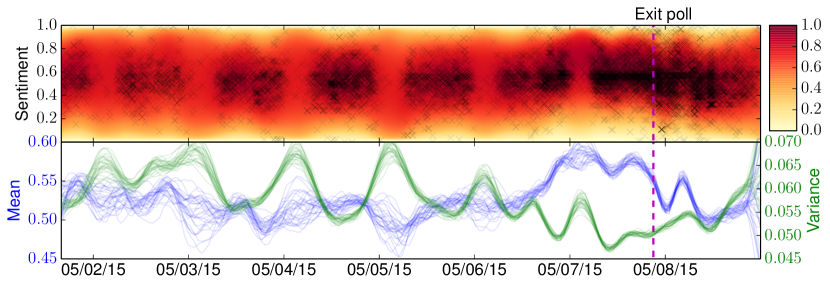
Figure 3: Twitter sentiment from the UK general election modelled using a heteroscedastic beta distribution. The timing of the exit poll is marked and is followed by a night of tweets as election counts come in. Other night time periods have a reduced volume of tweets and a corresponding increase in sentiment variance. Ticks on the x-axis indicate midnight.

4.2.1 Survival Analysis

Survival analysis focuses on the analysis of time-to-event data. This data arises frequently in clinical trials, though it is also commonly found in failure tests within engineering. In these settings it is common to observe censoring. Censoring occurs when an event is only observed to exist between two times, but no further information is available. For right-censoring, the most common type of censoring, the event time $T\in[t,\infty)$.

A common model to analyse this type of data is an accelerated failure time model. This suggests that the distribution of when an random event, $T$, may occur, is multiplicatively effected by some function of the covariates, $f(\mathbf{x})$, thus accelerating or retarding time; akin to notion of dog years. In a generalized linear model we may write this as $\log T=\log T_{0}+\log f(\mathbf{x})$, where $T$ is the random variable for failure time of the individual with covariates $\mathbf{x}$, and $T_{0}$ follows a parametric distribution describing a non-accelerated failure time.

To account for censoring the cumulative distribution needs to be computable and event times are restricted to be positive. A common parametric distribution for $T_{0}$ that fulfills these restrictions is the log-logistic distribution, with the median being some function of the covariates, $f(\mathbf{x})$. This however is restrictive as the shape of failure time distribution is assumed to be the same for all patients. We relax this assumption by allowing the shape parameter of the log-logistic distribution to vary with response to the input,

$$y_{i}\sim LL(\alpha=e^{f(\mathbf{x}_{i})},\beta=e^{g(\mathbf{x}_{i})}),$$

where $f(\mathbf{x})=\mathcal{GP}({\bm{\mu}}_{f},k_{f}(\mathbf{x},\mathbf{x}^{\prime}))$ and $g(\mathbf{x})=\mathcal{GP}({\bm{\mu}}_{g},k_{g}(\mathbf{x},\mathbf{x}^{\prime}))$. This allows both skewed unimodal and exponential shaped distributions for the failure time distribution depending on the individual, as shown in Figure 4. Again there is no associated link-function in this case, and the model can be modelled as a chained-survival model.

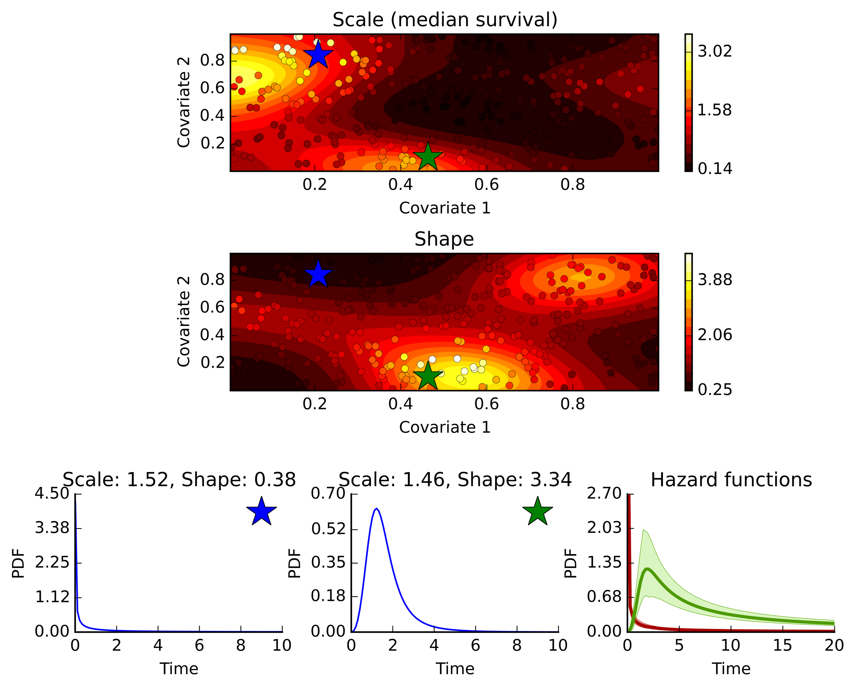
Figure 4: Resulting model on synthetic survival dataset. Shows variation of median survival time and shape of log-logistic distribution, in response to differing covariate information. Background colour shows the chained-survivals predictions, coloured dots show ground truth. Lower figures show associated failure time distributions and hazards for two different synthetic patients. Shapes can be both unimodal or exponential.

Data	NLPD
	G	LSurv	VSurv	CHSurv
leuk	$4.03\pm.08$	$1.57\pm.01$	$1.57\pm.01$	$1.56\pm.01$
Surv	$5.45\pm.06$	$2.52\pm.02$	$2.52\pm.02$	$2.16\pm.02$

Table 2: Results NLPD over 5 cross-validation folds with 10 replicates each. Models shown in comparison are sparse Gaussian (G), survival Laplace approximation (LSurv), survival VB approximation (VSurv), chained heteroscedastic survival (CHSurv).

Table 2 shows the models performance a real and synthetic datasets. The leukemia dataset (Henderson et al., 2002) contains censored event times for 1043 leukemia patients and is known to have non-linear responses certain covariates (Gelman et al., 2013). We find little advantage from using the chained-survival model, but as usual the model is robust such that performance isn’t degraded in this case. We additionally show the results on a synthetic dataset where the shape parameter is known to vary with response to the input, in this case an increase in performance is seen. See Appendix A.5 for more details on the model and synthetic dataset.

4.2.2 Twitter Sentiment Analysis in the UK Election

The final experiment shows the adaptability of the model even further, on a novel dataset and with a novel heteroscedastic model. We consider sentiment in the UK general election, focussing on tweets tagged as supporters of the Labour party. We used a sentiment analysis tagging system to evaluate the positiveness of 105,396 tweets containing hashtags relating to recent the major political parties, over the run in to the UK 2015 general election.

We are interested in modeling the distribution of positive sentiment as a function of time. The sentiment value is constrained to be to be between zero and one, and we do not believe the distribution of tweets through time to be necessarily unimodal. A natural likelihood to use in this case is the beta likelihood. This allows us to accommodate bathtub shaped distributions, indicating tweets are either extremely positive or extremely negative. We then allow the distribution over tweets to be heterogenous throughout time by using Gaussian process models for each parameter of the beta distribution,

$$y_{i}\sim B(\alpha=e^{f(\mathbf{x}_{i})},\beta=e^{g(\mathbf{x}_{i})}),$$

where $f(\mathbf{x})=\mathcal{GP}({\bm{\mu}}_{f},k_{f}(\mathbf{x},\mathbf{x}^{\prime}))$ and $g(\mathbf{x})=\mathcal{GP}({\bm{\mu}}_{g},k_{g}(\mathbf{x},\mathbf{x}^{\prime}))$.

The upper section of Figure 3 shows the data and the probability of each sentiment value throughout time. The lower part shows the corresponding mean and variance functions induced by the above parameterization. This year’s general election was particularly interesting: polls throughout the election showed it to be a close race between the two major parties, Conservative and Labour. But at the end of polling an exit poll was released that predicted an outright win for the Conservatives. This exit poll proved accurate and is associated with a corresponding dip in the sentiment of the tweets. Other interesting aspects of the analysis include the reduction in number of tweets during the night and the corresponding increase in the variance of our estimates.

4.2.3 Decomposition of Poisson Processes

The intensity, $\lambda(x)$, of a Poisson process can be modelled as the product of two positive latent functions, $\exp(f(x))$ and $\exp(g(x))$, as a generalrised linear model,

$$\log(\lambda)=f(x)+g(x)$$

$$y\sim\textrm{Poisson}(\lambda=\exp(f+g)=\exp(f(x))\exp(g(x))),$$

using a log link function.

Instead imagine we form a new process by combining two different underlying Poisson processes through addition. The superposition property of Poissons means that the resulting process is also Poisson with rates given by the sum of the underlying rates.

To model this via a Gaussian process we have to assume that the intensity of the resulting Poisson, $\lambda(x)$ is a sum of two positive functions, which are denoted by $\exp(f(x))$ and $\exp(g(x))$ respectively,

$$y\sim\textrm{Poisson}(\lambda=\exp(f(x))+\exp(g(x))),$$ (10)

there is no link function representation for this model, it takes the form of a chained-GP.

Focusing purely on the generative model of the data, the lack of an link function does not present an issue. Figure 5 shows a simple demonstration of the idea in a simulated data set.

Using an additive model for the rate rather than a multiplicative model for counting processes has been discussed previously in the context of linear models for survival analysis, with promising results Lin and Ying (1995).

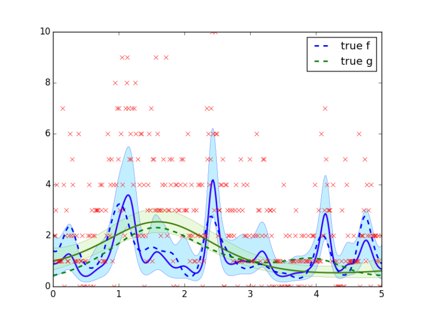
Figure 5: Even with 350 data we can start to see the differentiation of the addition of a long lengthscale positive process and a short lengthscale positive process. Red crosses denote observations, dotted lines are the true latent functions generating the data using Eq (10), the solid line and associated error bars are the approximate posterior predictions, $q({\bf f}^{*}),q({\bf g}^{*})$, of the latent processes.

To illustrate the model on real data we considered homicide data in Chicago. Taking data from http://homicides.redeyechicago.com/ (see also Linderman and Adams (2014)) we aggregated data into three months periods by zip code. We considered an additive Poisson process with a particular structure for the covariance functions. We constructed a rate of the form:

$$\Lambda(x,t)=\lambda_{1}(x)\mu_{1}(t)+\lambda_{2}(x)\mu_{2}(t)$$

where $\lambda_{1}(x)=\exp(f_{1}(x))$, $\lambda_{2}(x)=\exp(g_{1}(x))$, $\mu_{1}(t)=\exp(f_{2}(t))$ and $\mu_{2}(t)=\exp(g_{2}(t))$ where $f_{1}(x)$, $g_{1}(x)$ are spatial GPs and $f_{2}(t)$ and $g_{2}(t)$ are temporal GPs. The overall rate decomposes into two separable rate functions, but the overall rate function is not separable. We have a sum of separable (Álvarez et al., 2012) rate functions. This structure allows us to decompose the homicide map into separate spatial maps that each evolve at different time rates. We selected one spatial map with a length scale of 0.04 and one spatial map with a length scale of 0.09. The time scales and variances of the temporal rate functions were optimized by maximum likelihood. The results are shown in Figure 6. The long length scale process hardly fluctuates across time, whereas the short lengthscale process, which represents more localized homicide activity, fluctuates across the seasons with scaled increases of around 1.25 deaths per month per zip code. This decomposition is possible and interpretable due to the structured underlying nature of the GPs inside the chained model.

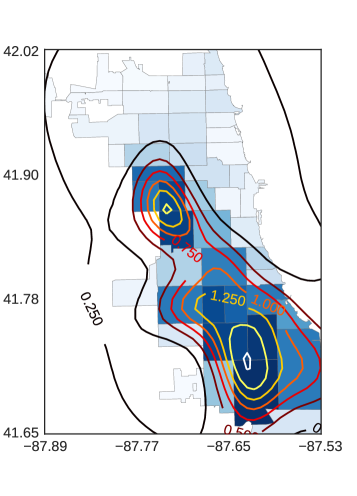
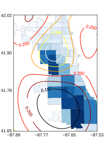
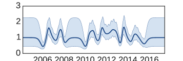
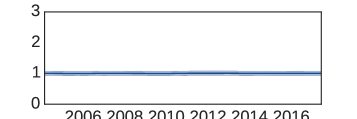
Figure 6: Homicide rate maps for Chicago. The short length scale spatial process, $\lambda_{1}(x)$ (above-left) is multiplied in the model by a temporal process, $\mu_{1}(t)$ (below-left) which fluctuates with passing seasons. Contours of spatial process are plotted as deaths per month per zip code area. Error bars on temporal processes are at 5th and 95th percentile. The longer length scale spatial process, $\lambda_{2}(x)$ (above-right) has been modeled with little to no fluctuation temporally $\mu_{2}(t)$ (below-right).

5 Conclusions

We have introduced “Chained Gaussian Process” models. They allow us to make predictions which are based on a non-linear combination of underlying latent functions. This gives a far more flexible formalism than the generalized linear models that are classically applied in this domain.

Chained Gaussian processes are a general formalism and therefore are intractable in the base case. We derived an approximation framework that is applicable for any factorized likelihood. For the cases we considered, involving two latent functions, the approximation made use of two dimensional Gauss-Hermite quadrature. We speculated that when the idea is extended to higher numbers of latent functions it may be necessary to resort to Monte Carlo sampling.

Our approximation is highly scalable through the use of stochastic variational inference. This enables the full range of standard stochastic optimizers to be applied in the framework.

Acknowledgments

AS was supported by a University of Sheffield, Faculty Scholarship, JH was supported by a MRC fellowship. The authors also thank Amazon for a donation of AWS compute time and the anonymous reviewers of a previous transcript of this work.

A Supplementary Material

A.1 Collapsed Heteroscedastic

Lazaro-Gredilla and Titsias (2011) form a bound by ‘collapsing out’ the $q({\bf f})$ distribution, such that it need not take a Gaussian form. As a brief review their bound can be derived as follows.

$$\log p(\mathbf{y}|{\bf f}) \geq{\mathbb{E}}_{q({\bf f})}\Big{[}{\log p(\mathbf{y}|{\bf f},{\bf g})}\Big{]}+\log{\mathbb{E}}_{q({\bf g})}\Big{[}{\frac{p({\bf g})}{q({\bf g})}}\Big{]}$$

$$=\log\mathcal{N}\left(\mathbf{y}|{\bf f},e^{{{\bm{m}}_{f}}_{i}-\frac{{{\bm{v}}_{f}}_{i}}{2}}\right)-\frac{1}{4}\sum^{n}_{i=1}{{\bm{v}}_{f}}_{i}=L^{\prime}$$

$$L =\int p(\mathbf{y}|{\bf f})p({\bf f})d{\bf f}$$

$$\geq\int e^{L^{\prime}}p({\bf f})d{\bf f}$$

$$=\int\mathcal{N}\left(\mathbf{y}|{\bf f},e^{{{\bm{m}}_{f}}_{i}-\frac{{{\bm{v}}_{f}}_{i}}{2}}\right)\mathcal{N}\left({\bf f}|0,\mathbf{{K}}_{{\bf f}{\bf f}}\right)-\frac{1}{4}\sum^{n}_{i=1}{{\bm{v}}_{f}}_{i}$$

$$\quad-\text{KL}\left(q({\bf g})\,\|\,p({\bf g})\right)$$

$$=\mathcal{N}\left(\mathbf{y}|0,\mathbf{{K}}_{{\bf f}{\bf f}}+e^{{{\bm{m}}_{f}}_{i}-\frac{{{\bm{v}}_{f}}_{i}}{2}}\right)-\frac{1}{4}\sum^{n}_{i=1}{{\bm{v}}_{f}}_{i}$$

$$\quad-\text{KL}\left(q({\bf g})\,\|\,p({\bf g})\right)$$

The bound that we assumes a sparse approximation, however it also constrains $q({\bf f})$ to be Gaussian. This leads to an additional KL divergence since the optimal is not chosen, and additional penalty term arising from the mismatch of the constrained form of $q({\bf f})$.

A.2 Quadrature and Monte Carlo

Computing the expected likelihood requires many low-dimensional integrals. Recently, there has been progress in using stochastic methods to obtain unbiased estimates in this area using centered representations (Kingma and Welling, 2014; Rezende et al., 2014). In this section, we re-examine the effectiveness of Gauss-Hermite quadrature in this setting. Gauss-Hermite quadrature approximates Gaussian integrals in one dimension using a pre-defined grid. For expectations of polynomial functions, the method is exact when the grid size meets the degree of the polynomial; for non-polynomial functions as we will encounter in general, we must accept a small amount of bias. To integrate higher dimensional functions, we must nest the quadrature, doing an integral across one dimension for each quadrature point in the other. Our experiments suggest that even in this case, the amount of bias is negligible, as Figure 7 investigates, examining the accuracy of nested quadrature as compared to Monte Carlo estimates using the centered parameterization (Kingma and Welling, 2014). Inspired by an examination of quadrature for expectation propagation (Jylänki et al., 2011), we examine the effectiveness for a several positions of the integral of a Student-$t$.

(a) Test locations marked

(b) Student-$t$ mode

(c) Student-$t$ shoulder

(d) Student-$t$ tail

Figure 7: Two dimensional Gauss-Hermite quadrature vs Monte Carlo. Each plot shows the log absolute error in estimating the two dimension integral required by our Heteroscedastic Student-$t$ model (see section 4.2). In each case, the bias introduced by quadrature (circles) is small: a long way into the tail of the variance from the MC approximation. In fact, for small numbers of quadrature points, we often do better than the expected value using many more MC samples. Boxplots shows the absolute error on 1000 separate reruns of MC, whereas quadrature is deterministic. The error was evaluated at various points in the tail of the distribution as shown in 7).

Gauss-Hermite quadrature is appropriate for our integral as the Gaussian posteriors $q({\bf f}_{i})q({\bf g}_{i})$ are convolved with a function $p(\mathbf{y}_{i}|{\bf g}_{i},{\bf f}_{i})$. Monte Carlo integration is exact in the limit of infinite samples, however in practice a subset of samples must be used. Gauss-Hermite requires ${p}h^{b}$ evaluations per point in the mini-batch, where $h$ is the number of Gauss-Hermite points used, $p$ is the number of output dimensions, and $b$ is the number of latent functions. Since Monte Carlo is unbiased, using a stochastic optimizer with the stochastic estimates of the integral and its gradients will work effectively (Nguyen and Bonilla, 2014; Kingma and Welling, 2014), though we find the bias introduced by the quadrature approach to be negligible. For higher number of latent functions it may be more efficient to make use of low variance Monte Carlo estimates for the integrals. Gradients for the model can be computed in a similar way with the Gaussian idenities used by Opper and Archambeau (2009).

A.3 Gradients and Optimization

Gradients can be computed similarly to (Hensman et al., 2015) using the equalities,

$$\frac{\partial}{\partial\mu}{\mathbb{E}}_{\mathcal{N}\left(x|\mu,\sigma^{2}\right)}\Big{[}{f(x)}\Big{]} ={\mathbb{E}}_{\mathcal{N}\left(x|\mu,\sigma^{2}\right)}\Big{[}{\frac{\partial}{\partial x}f(x)}\Big{]}$$ (11)

$$\frac{\partial}{\partial\sigma^{2}}{\mathbb{E}}_{\mathcal{N}\left(x|\mu,\sigma^{2}\right)}\Big{[}{f(x)}\Big{]} =\frac{1}{2}{\mathbb{E}}_{\mathcal{N}\left(x|\mu,\sigma^{2}\right)}\Big{[}{\frac{\partial}{\partial x^{2}}f(x)}\Big{]}$$ (12)

and the chain rule.

Since our posterior assumes factorization between $q({\bf f})$ and $q({\bf g})$ we simply do the gradients independently. That is calculate

$$\frac{\partial}{\partial{\bm{\mu}}_{f}}{\mathbb{E}}_{\mathcal{N}\left(\mathbf{x}_{i}|{{\bm{m}}_{f}},{{\bm{v}}_{f}}\right)}\Big{[}{\log p(\mathbf{y}|{\bf f},{\bf g})}\Big{]}$$

$$\frac{\partial}{\partial{\bm{\mu}}_{g}}{\mathbb{E}}_{\mathcal{N}\left(\mathbf{x}_{i}|{{\bm{m}}_{g}},{{\bm{v}}_{g}}\right)}\Big{[}{\log p(\mathbf{y}|{\bf f},{\bf g})}\Big{]}$$

$$\frac{\partial}{\partial{{\bm{v}}_{f}}}{\mathbb{E}}_{\mathcal{N}\left(\mathbf{x}_{i}|{{\bm{m}}_{f}},{{\bm{v}}_{f}}\right)}\Big{[}{\log p(\mathbf{y}|{\bf f},{\bf g})}\Big{]}$$

$$\frac{\partial}{\partial{{\bm{v}}_{g}}}{\mathbb{E}}_{\mathcal{N}\left(\mathbf{x}_{i}|{{\bm{m}}_{g}},{{\bm{v}}_{g}}\right)}\Big{[}{\log p(\mathbf{y}|{\bf f},{\bf g})}\Big{]},$$

independently using (11) and (12). The expectations can then be done using quadrature, or Monte Carlo sampling. As before

$${{\bm{m}}_{f}} =\mathbf{{K}}_{{\bf f}{\bf u}_{f}}\mathbf{{K}}_{{\bf u}_{f}{\bf u}_{f}}^{-1}{\bm{\mu}}_{f}$$

$${{\bm{v}}_{f}} =\mathbf{{K}}_{{\bf f}{\bf f}}+\mathbf{{K}}_{{\bf f}{\bf u}_{f}}\mathbf{{K}}_{{\bf u}_{f}{\bf u}_{f}}^{-1}({\bm{S}}_{f}-\mathbf{{K}}_{{\bf u}_{f}{\bf u}_{f}})\mathbf{{K}}_{{\bf u}_{f}{\bf u}_{f}}^{-1}\mathbf{{K}}_{{\bf u}_{f}{\bf f}}$$

$${{\bm{m}}_{g}} =\mathbf{{K}}_{{\bf g}{\bf u}_{g}}\mathbf{{K}}_{{\bf u}_{g}{\bf u}_{g}}^{-1}{\bm{\mu}}_{g}$$

$${{\bm{v}}_{g}} =\mathbf{{K}}_{{\bf g}{\bf g}}+\mathbf{{K}}_{{\bf g}{\bf u}_{g}}\mathbf{{K}}_{{\bf u}_{g}{\bf u}_{g}}^{-1}({\bm{S}}_{g}-\mathbf{{K}}_{{\bf u}_{g}{\bf u}_{g}})\mathbf{{K}}_{{\bf u}_{g}{\bf u}_{g}}^{-1}\mathbf{{K}}_{{\bf u}_{g}{\bf g}}.$$

We then can chain using $\frac{\partial}{\partial{{\bm{m}}_{f}}}{\mathbb{E}}_{\mathcal{N}\left(\mathbf{x}_{i}|{{\bm{m}}_{f}},{{\bm{v}}_{f}}\right)}\Big{[}{\log p(\mathbf{y}|{\bf f},{\bf g})}\Big{]}\frac{\partial{{\bm{m}}_{f}}}{\partial\mathbf{{K}}_{{\bf f}{\bf u}_{f}}}\frac{\partial\mathbf{{K}}_{{\bf f}{\bf u}_{f}}}{\partial\theta}$, where $\theta$ is a hyper parameter of the kernel $k_{f}$. Similar chain rules can be written for the other derivatives.

The model contains variational parameters corresponding to $q({\bf u}_{f})=\mathcal{N}\left({\bf u}_{f}|{\bm{\mu}}_{f},{\bm{S}}_{f}\right)$ and $q({\bf u}_{g})=\mathcal{N}\left({\bf u}_{g}|{\bm{\mu}}_{g},{\bm{S}}_{g}\right)$ and the latent input locations, $\mathbf{{Z}}$. As such the parameters do not scale with $n$. Naively the number of parameters is $\mathcal{O}(b(m^{2}+m)+m)$ however we can reduce this to $\mathcal{O}(b(\frac{m^{2}}{2}+m))$ by parameterizing the Choleksy of the covariance matrices, ${\bm{S}}_{f}=L_{{\bf f}}L_{{\bf f}}^{\top}$ and ${\bm{S}}_{g}=L_{{\bf g}}L^{\top}_{{\bf g}}$. This has the added benefit of enforcing that ${\bm{S}}_{f}$ and ${\bm{S}}_{g}$ are symmetrical and positive definite.

We initialize the model with random or informed lengthscales within the right region, ${\bm{\mu}}_{f}$ and ${\bm{\mu}}_{g}$ are assigned small random values, ${\bm{S}}_{g}$ and ${\bm{S}}_{f}$ are given an identity form. In practice during optimization we find it helpful to initially fix all the kernel hyperparameters and $\mathbf{{Z}}$ at their initial locations, optimize for a small number of steps, then allow the optimization to run freely. This allows the latent means ${\bm{\mu}}_{f}$ and ${\bm{\mu}}_{g}$ to move to sensible locations before the model is allowed to completely change the form of the function through the modification of the kernel hyperparameters. True convergence can be difficult to achieve due to the potentially number of strongly dependent parameters and the non-convex optimization problem, and in practice we find it helpful to monitor convergence. It is important to note however that the number of parameters to be optimized is fixed with respect to $n$.

A.4 Further Twitter experiment details

The model used to model the twitter data has some interesting properties, such as the ability to model a transition from a unimodal distribution to a bimodal distribution. The following plot shows how the distribution changes throughout time for the Labour dataset.

The latent functions $\alpha$ and $\beta$ which are modelled in Section 4.2.2 can be plotted themselves. If both latent functions went below $1.0$ then the distribution at that time would turn into a bathtub shape. If both are larger than one but one is larger than the other, we have a skewed distribution. If one is below zero and the over above, it appears exponential or negative exponential.

A.5 Survival details

To generate the synthetic survival dataset we first define latent functions that we wish to infer. These are a complex function of an input, $\mathbf{x}$, with two dimensions,

$$\mathbf{\alpha} =\exp\left(2\exp(-30(\mathbf{x}_{:,0}-\frac{1}{4})^{2})+\sin(\pi\mathbf{x}_{:,1}^{2})-2\right)$$

$$\mathbf{\beta} =\exp\left(\sin(2\pi\mathbf{x}_{:,0})+\cos(2\pi\mathbf{x}_{:,1})\right).$$

We then make 1000 synthetic individuals, with covariates sampled uniformly from $\mathbf{x}_{i,0}\sim\text{Uniform}(0,1)$ and $\mathbf{x}_{i,1}\sim\text{Uniform}(0,1)$.

Using these two latent functions, $\mathbf{\alpha}_{i}$ and $\mathbf{\beta}_{i}$, computed using covariates $\mathbf{x}_{i}$ for individual $i$, we sample a simulated failure time from a log-logistic distribution,

$$\mathbf{y}\sim LL(\mathbf{\alpha},\mathbf{\beta})=\frac{\left(\frac{\mathbf{\beta}}{\alpha}\right)\left(\frac{\mathbf{y}}{\alpha}\right)^{\mathbf{\beta}-1}}{\left(1+\frac{\mathbf{y}}{\alpha}^{\mathbf{\beta}}\right)^{2}}.$$

These are then the true failure times of individuals with covariates $\mathbf{x}_{i}$. $20\%$ of the data is chosen to be censored censor. A time is uniformly drawn, and the observed time is truncated to this time, $\mathbf{y}_{i}=\mathbf{t}_{i}$. Otherwise $\mathbf{t}_{i}=\mathbf{y}_{i}$. Additionally a indicator $\mathbf{\delta}_{i}=1$ is provided to the model if censoring occurs, and $\mathbf{\delta}_{i}=0$ if the real failure time was observed. This mimics patients dropping out of a trial, with the assumption that the time at which they drop out is independent of the failure time and covariates. For these censored times, we only know that $\mathbf{T}_{i}>\mathbf{t}_{i}$, and for the uncensored individuals it is known that $\mathbf{T}_{i}=\mathbf{t}_{i}$.

As such the likelihood is decomposed into $P(t_{i}\leq\mathbf{y}_{i}<\mathbf{t}_{i}+\delta t|\mathbf{\alpha}_{i},\mathbf{\beta}_{i},\mathbf{\delta}_{i}=0)$ and $P(\mathbf{y}_{i}|\mathbf{\alpha}_{i},\mathbf{\beta}_{i},\mathbf{\delta}_{i}=1)=1-P(\mathbf{y}_{i}>\mathbf{t}_{i}|\mathbf{\alpha}_{i},\mathbf{\beta}_{i},\mathbf{\delta}_{i}=1)$

$$p(\mathbf{y}|\mathbf{\alpha},\mathbf{\beta},\mathbf{\delta})=\prod^{K:\delta\neq 1}_{i}\frac{\left(\frac{\mathbf{\beta}_{i}}{\alpha_{i}}\right)\left(\frac{\mathbf{y}_{i}}{\alpha_{i}}\right)^{\mathbf{\beta}_{i}-1}}{\left(1+\frac{\mathbf{y}_{i}}{\alpha_{i}}^{\mathbf{\beta}_{i}}\right)^{2}}\prod^{M:\delta=1}_{j}\frac{1}{1+\left(\frac{\mathbf{y}_{j}}{\alpha_{j}}\right)^{\mathbf{\beta}_{j}}}$$

The task is then to infer $\mathbf{\alpha}$ and $\mathbf{\beta}$, such that we know how the failure time distribution varies in response to covariate information.

References

- Adams and Stegle (2008) Ryan Prescott Adams and Oliver Stegle. Gaussian process product models for nonparametric nonstationarity. In Proceedings of the 25th International Conference on Machine Learning, pages 1–8, 2008.
- Álvarez et al. (2012) Mauricio Álvarez, Lorenzo Rosasco, and Neil D. Lawrence. Kernels for vector-valued functions: A review. Foundations and Trends in Machine Learning, 4(3):195–266, 2012. doi: 10.1561/2200000036.
- Dezfouli and Bonilla (2015) Amir Dezfouli and Edwin V Bonilla. Scalable inference for Gaussian process models with black-box likelihoods. In C. Cortes, N. D. Lawrence, D. D. Lee, M. Sugiyama, and R. Garnett, editors, Advances in Neural Information Processing Systems 28, pages 1414–1422. Curran Associates, Inc., 2015.
- Duchi et al. (2011) John Duchi, Elad Hazan, and Yoram Singer. Adaptive subgradient methods for online learning and stochastic optimization. J. Mach. Learn. Res., 12:2121–2159, July 2011. ISSN 1532-4435.
- Gal et al. (2014) Yarin Gal, Mark van der Wilk, and Carl E. Rasmussen. Distributed variational inference in sparse Gaussian process regression and latent variable models. In Zoubin Ghahramani, Max Welling, Corinna Cortes, Neil D. Lawrence, and Kilian Q. Weinberger, editors, Advances in Neural Information Processing Systems, volume 27, Cambridge, MA, 2014.
- Gelman et al. (2013) Andrew Gelman, John B. Carlin, Hal S. Stern, David B. Dunson, Aki Vehtari, and Donald B. Rubin. Bayesian Data Analysis, Third Edition. CRC Press, November 2013. ISBN 9781439840955.
- Goldberg et al. (1998) Paul W. Goldberg, Christopher K. I. Williams, and Christopher M. Bishop. Regression with input-dependent noise: A Gaussian process treatment. In Michael I. Jordan, Michael J. Kearns, and Sara A. Solla, editors, Advances in Neural Information Processing Systems, volume 10, pages 493–499, Cambridge, MA, 1998. MIT Press.
- Henderson et al. (2002) R. Henderson, S. Shimakura, and Gorst D. Modeling spatial variation in leukemia survival data. Journal of the American Statistical Association, 97:965–972, 2002.
- Hensman et al. (2013a) James Hensman, Nicoló Fusi, and Neil D. Lawrence. Gaussian processes for big data. In Ann Nicholson and Padhraic Smyth, editors, Uncertainty in Artificial Intelligence, volume 29. AUAI Press, 2013a.
- Hensman et al. (2013b) James Hensman, Neil D. Lawrence, and Magnus Rattray. Hierarchical Bayesian modelling of gene expression time series across irregularly sampled replicates and clusters. BMC Bioinformatics, 14(252), 2013b. doi: doi:10.1186/1471-2105-14-252.
- Hensman et al. (2015) James Hensman, Alexander G D G Matthews, and Zoubin Ghahramani. Scalable variational Gaussian process classification. In In 18th International Conference on Artificial Intelligence and Statistics, pages 1–9, San Diego, California, USA, May 2015.
- Hernández-Lobato et al. (2014) Daniel Hernández-Lobato, Viktoriia Sharmanska, Kristian Kersting, Christoph H Lampert, and Novi Quadrianto. Mind the nuisance: Gaussian process classification using privileged noise. In Z. Ghahramani, M. Welling, C. Cortes, N.D. Lawrence, and K.Q. Weinberger, editors, Advances in Neural Information Processing Systems 27, pages 837–845. Curran Associates, Inc., 2014.
- Hoffman et al. (2013) Matthew D. Hoffman, David M. Blei, Chong Wang, and John Paisley. Stochastic variational inference. Journal of Machine Learning Research, 14:1303–1347, 2013.
- Jylänki et al. (2011) Pasi Jylänki, Jarno Vanhatalo, and Aki Vehtari. Robust Gaussian process regression with a Student-t likelihood. J. Mach. Learn. Res., 12:3227–3257, November 2011. ISSN 1532-4435.
- Kingma and Welling (2014) D. P. Kingma and M. Welling. Stochastic gradient VB and the variational auto-encoder. In 2nd International Conference on Learning Representations (ICLR), Banff, 2014.
- Kuß (2006) Malte Kuß. Gaussian Process Models for Robust Regression, Classification, and Reinforcement Learning. PhD thesis, TU Darmstadt, April 2006.