The Poincaré-Bendixson Theorem and the Non-linear Cauchy-Riemann Equations

Abstract

In [6] Fiedler and Mallet-Paret prove a version of the classical Poincaré-Bendixson Theorem for scalar parabolic equations. We prove that a similar result holds for bounded solutions of the non-linear Cauchy-Riemann equations. The latter is an application of an abstract theorem for flows with a(n) (unbounded) discrete Lyapunov function.

1 Introduction

The classical Poincaré-Bendixson Theorem describes the asymptotic behavior of flows in the plane. The topology of the plane puts severe restrictions on the behavior of limit sets. The Poincaré-Bendixson Theorem states for example that if the $\alpha$- and the $\omega$-limit set of a bounded trajectory of a smooth flow in ${\mathbb{R}}^{2}$ does not contain equilibria, then the limit set is a periodic orbit. Several generalizations of this theorem have appeared in the literature. For instance the generalization of the Poincaré-Bendixson Theorem to two-dimensional manifolds, cf. [3]. In [7] an extension to continuous (two-dimensional) flows is obtained and [4] provides a generalization to semi-flows. The remarkable result by Fiedler and Mallet-Paret [6] establishes an extension of the Poincaré-Bendixson Theorem to infinite dimensional dynamical systems with a positive Lyapunov function. They apply their result to scalar parabolic equations of the form

$$u_{s}=u_{xx}+f(x,u,u_{x}),\quad x\in S^{1},f\in C^{2}.$$ (1.1)

In this paper we establish a version of the Poincaré-Bendixson Theorem for bounded orbits of the nonlinear Cauchy-Riemann equations in the plane. A bounded orbit of the nonlinear Cauchy-Riemann equations is a (smooth) bounded function $u\colon{\mathbb{R}}\times S^{1}\to{\mathbb{R}}^{2}$, which satisfies

$$u_{s}-J\bigl{(}u_{t}-F(t,u)\bigr{)}=0,$$ (1.2)

with $u(s,t)=\bigl{(}p(s,t),q(s,t)\bigr{)}$, $s\in{\mathbb{R}}$, $t\in S^{1}={\mathbb{R}}/{\mathbb{Z}}.$ Here $F(t,u)$ is a smooth non-autonomous vector field on ${\mathbb{R}}^{2}$ and $J$ is the symplectic matrix

$$J=\left(\begin{array}[]{cc}0&-1\\ 1&0\end{array}\right).$$

We prove that the asymptotic behavior, as $s$ goes to infinity, of bounded solutions of Equation (1.2) is as simple as the limiting behavior of flows in ${\mathbb{R}}^{2}.$ Equation (1.2) arises in many different contexts, in particular in Floer homology literature, where the vector field has the form $F(t,u)=F_{H}(t,u),$ i.e. $F_{H}$ is Hamiltonian, cf.  [9]. The latter implies that there exists a time-dependent Hamiltonian function $H(t,\cdot):{\mathbb{R}}^{2}\to{\mathbb{R}}$, such that $F_{H}(t,u)=J\nabla H(t,u)$. In the Hamiltonian case the Cauchy-Riemann equations are the $L^{2}$-gradient flow of the Hamilton action and as such bounded solutions of (1.2) will, generically, be connections orbits between equilibria. The Hamilton action is an ${\mathbb{R}}$-valued Lyapunov function for the Cauchy-Riemann equations. In this paper we obtain a result about the asymptotic behavior of orbits for general vector fields $F$ in the Cauchy-Riemann equations.

A bounded solution of the Cauchy-Riemann equations is a smooth function $u$ with $|u(s,t)|\leq C$. Let $X$ be the set of solutions bounded by a fixed (but arbitrary) constant (in the present work we will always choose $C=1$). Endowed with the compact-open topology $X$ is a compact Hausdorff space. The translation invariance of the Cauchy-Riemann equations in the $s-$variable defines an induced flow on $X$ by translating solutions in the $s$-variable. A bounded solution $u$ can be identified with its orbit $\gamma(u),$ and $\alpha(u)$ and $\omega(u)$ are well-defined elements of $X$. In Section 2 we given a detailed account of the space $X$ and the induced translation flow in the context of the Cauchy-Riemann equations.

Theorem 1.1.

Let $u$ be a bounded solution of the Cauchy-Riemann Equations (1.2). Then, for the $\omega$-limit set $\omega(u)$ the following dichotomy holds:

1. either $\omega(u)$ consists of exactly one $s$-periodic orbit, or

2. $\alpha(v)\subseteq E$ and $\omega(v)\subseteq E$, for every $v\in\omega(u)$,

where $E$ denotes the set of equilibria of Equation (1.2), i.e. the 1-periodic solutions of the vector field $F(t,x)$. The same dichotomy holds for the $\alpha$-limit set $\alpha(u)$.

As in the classical Poincaré-Bendixson Theorem alternative (ii) allows for $\omega(u)$ (or $\alpha(u)$) to consist of homoclinic and heteroclinic solutions joining equilibria. An important reason why a generalization of the Poincaré-Bendixson holds for the Cauchy-Riemann equations is that there exists a continuous projection onto ${\mathbb{R}}^{2}$, which is defined as follows. Let $t_{0}\in S^{1}$ be arbitrary, then define

$$\begin{array}[]{lccl}\pi_{t_{0}}:&X&\to&{\mathbb{R}}^{2}\\ &u=(p,q)&\mapsto&\pi_{t_{0}}(u)=\bigl{(}p(0,t_{0}),q(0,t_{0})\bigr{)}.\end{array}$$ (1.3)

Theorem 1.2.

Under the assumptions of Theorem 1.1 the projection

$$\pi_{t_{0}}\colon\omega(u)\to\pi_{t_{0}}\omega(u)$$

is a homeomorphism onto its image.

In general, if a flow allows a continuous Lyapunov function, then limit sets of orbits consist only of equilibria. Such flows are referred to as gradient-like flows. Theorem 3.1 in this paper gives an abstract extension of the Poincaré-Bendixson Theorem to flows that allow a discrete Lyapunov function. In particular Theorem 3.1 implies Theorem 1.1. Note that Theorem 1.2 together with the classical Poincaré-Bendixson Theorem also implies Theorem 1.1. An abstract version of Theorem 1.2 is proved in Section 5.

The main differences between the results in [6] for parabolic equations and the results in this paper are that the Cauchy-Riemann equations do not define a well-posed initial value problem and, more importantly, the discrete Lyapunov functions that are considered in this paper are not bounded from below. Furthermore, the results obtained in this paper do not assume differentiability of the flow, nor does the flow need to be defined on a Banach space. We believe that most of the results in this paper extendable to semi-flows, e.g. [4].

In Section 2 we analyze the main properties of the Cauchy-Riemann equations (1.2) and additional details are given in Section 6. In Section 3 we set up an abstract setting which generalizes the properties of the Cauchy-Riemann equations. In Sections 4 and 5 a full proof of the Poincaré-Bendixson Theorem is given adapted to the abstract setting introduced in Section 3.

2 The Cauchy-Riemann Equations

The initial value problem of Equation (1.2) is ill-posed. Given an initial value $u(0,t)=u_{0}(t)$, there may not exist solutions $u(s,t)$ of Equation (1.2) for any $s$-time interval $I\ni 0$. We therefore restrict our attention to bounded solutions, which are functions $u\in C^{1}({\mathbb{R}}\times S^{1};{\mathbb{R}}^{2})$ that satisfy Equation (1.2) and for which

$$|u(s,t)|<\infty,\quad\text{for all }(s,t)\in{\mathbb{R}}\times S^{1}.$$ (2.1)

Since each bounded solution may be considered separately, it suffices to look at the space $X$ of functions $u\in C^{1}({\mathbb{R}}\times S^{1};{\mathbb{R}}^{2})$ satisfying Equation (1.2) and

$$|u(s,t)|\leq C,\quad\text{for all }(s,t)\in{\mathbb{R}}\times S^{1},$$

for some fixed arbitrary constant $C>0.$ Note that, without loss of generality, we can choose $C=1.$ On $X$ we consider the compact-open topology, i.e.

$$u^{n}\xrightarrow{X}u\quad\iff\quad u^{n}\xrightarrow{C^{0}_{\text{loc}}}u,$$ (2.2)

where the latter indicates uniform convergence on compact subsets of $S^{1}\times{\mathbb{R}}.$ Since $C^{0}({\mathbb{R}}\times S^{1};{\mathbb{R}}^{2})$, endowed with the compact-open topology, is Hausdorff (see [10, §47]), and $X\subset C^{0}({\mathbb{R}}\times S^{1};{\mathbb{R}}^{2})$, also $X$ is a Hausdorff space.

Proposition 2.1.

The solution space $X$ is a compact Hausdorff space.

Proof.

See Section 6. ∎

Identify the translation mapping $(s,t)\mapsto(s+\sigma,t)$ by $\sigma\in{\mathbb{R}}$ and consider the evaluation mapping

$${\mathbb{R}}\times C^{0}({\mathbb{R}}\times S^{1};{\mathbb{R}}^{2})\to C^{0}({\mathbb{R}}\times S^{1};{\mathbb{R}}^{2}),\quad(\sigma,u)\mapsto\phi^{\sigma}(u)=u\circ\sigma.$$ (2.3)

Lemma 2.2.

The evaluation mapping $(\sigma,u)\mapsto\phi^{\sigma}(u)$ is continuous with respect to the compact-open topology on $C^{0}({\mathbb{R}}\times S^{1};{\mathbb{R}}^{2})$.

Proof.

Since ${\mathbb{R}}\times S^{1}$ is a locally compact Hausdorff space, the composition of mappings

$$C^{0}({\mathbb{R}}\times S^{1};{\mathbb{R}}\times S^{1})\times C^{0}({\mathbb{R}}\times S^{1};{\mathbb{R}}^{2})\to C^{0}({\mathbb{R}}\times S^{1};{\mathbb{R}}^{2}),$$

is continuous with respect to the compact-open topologies on $C^{0}({\mathbb{R}}\times S^{1};{\mathbb{R}}\times S^{1})$ and $C^{0}({\mathbb{R}}\times S^{1};{\mathbb{R}}^{2})$, see [10, §46]. The translation $\sigma$ as defined above is a continuous mapping in $C^{0}({\mathbb{R}}\times S^{1};{\mathbb{R}}\times S^{1})$, which proves the lemma. ∎

Since the Cauchy-Riemann Equations are $s$-translation invariant, $u\in X$ implies that $\phi^{\sigma}(u)\in X.$ We therefore obtain a continuous mapping ${\mathbb{R}}\times X\to X$, again denoted by $\phi^{\sigma}(u)$. Also,

$$\phi^{\sigma}\bigl{(}\phi^{\sigma^{\prime}}(u)\bigr{)}=(u\circ\sigma^{\prime})\circ\sigma=u\circ(\sigma+\sigma^{\prime})=\phi^{\sigma+\sigma^{\prime}}(u),$$

which shows that $\phi^{\sigma}$ defines a continuous flow on $X$. A continuous flow on $X$ is a continuous mapping $(\sigma,u)\mapsto\phi^{\sigma}(u)\in X$, such that $\phi^{0}(u)=u$ and $\phi^{\sigma+\sigma^{\prime}}(u)=\phi^{\sigma}(\phi^{\sigma^{\prime}}(u))$, for all $\sigma,\sigma^{\prime}\in{\mathbb{R}}$ and for all $u\in X$.

Consider the evaluation mapping $\iota:C^{0}({\mathbb{R}}\times S^{1};{\mathbb{R}}^{2})\to C^{0}(S^{1};{\mathbb{R}}^{2})$, defined by

$$u(\cdot,\cdot)\mapsto u(0,\cdot).$$

By a similar argument as in Lemma 2.2 it follows that the mapping $\iota$ is a continuous mapping with respect to the compact-open topology on $C^{0}(S^{1};{\mathbb{R}}^{2}).$

Proposition 2.3.

The mapping $\iota:X\to{\mathscr{X}}$, with ${\mathscr{X}}=\iota(X)$, is a homeomorphism.

Proof.

See Section 6. ∎

For $\phi^{\sigma}$ we have the following commuting diagram:

$$\begin{diagram}$$

with $u(0,\cdot)\mapsto T^{\sigma}(u(0,\cdot))=u(\sigma,\cdot)$, and $T^{\sigma}$ defines a flow on ${\mathscr{X}}$.

The principal tool in the proof of Theorem 1.1 is the existence of an unbounded, discrete Lyapunov function, which decreases along orbits of the flow $\phi^{\sigma}.$ Let $u^{1},u^{2}\in X$ be two solutions, with $u^{1}\not=u^{2}$, such that the function $t\mapsto u^{1}(s,t)-u^{2}(s,t)$ is nowhere zero. Then define $w:=u^{1}-u^{2}\in C^{0}({\mathbb{R}}\times S^{1};{\mathbb{R}}^{2}).$ The $s$-dependent winding number ${\mathscr{W}}$ of the pair $(u^{1},u^{2})$ is defined as the winding number of $w$ about the origin, i.e.

$${\mathscr{W}}\bigl{(}u^{1}(s,\cdot),u^{2}(s,\cdot)\bigr{)}:={\mathscr{W}}(w(s,\cdot),0)=\frac{1}{2\pi}\int_{S^{1}}w^{*}\theta,$$ (2.4)

where $\theta=\frac{-qdp+pdq}{p^{2}+q^{2}}$ is a closed one-form on ${\mathbb{R}}^{2}\setminus\{0\}$, cf.  [11]. A pair of solutions $(u^{1},u^{2})\in X\times X$ is said to be singular if they belong to the “crossing” set defined by

$$\Sigma_{X}:=\{(u^{1},u^{2})\in X\times X:\exists~{}s\in{\mathbb{R}}\ :\ u^{1}(s,t)=u^{2}(s,t)\ \text{for some }t\in S^{1}\}.$$

The Lyapunov function $W\colon(X\times X)\setminus\Sigma_{X}\to{\mathbb{Z}}$ is defined by

$$W(u^{1},u^{2}):={\mathscr{W}}\bigl{(}\iota(u^{1}),\iota(u^{2})\bigr{)}.$$ (2.5)

The Lyapunov function $W$ is continuous on $(X\times X)\setminus\Sigma_{X}$ and constant on connected components. The set $\Sigma_{X}$ is a closed in $X\times X,$ since uniform convergence on compact sets implies point-wise convergence. The Lyapunov function $W$ is a symmetric:

$$W(u^{1},u^{2})=W(u^{2},u^{1}),\ \ \ \ \ \text{for all}\ (u^{1},u^{2})\not\in\Sigma_{X}.$$

The diagonal in $X\times X$ is defined by

$$\Delta:=\{(u^{1},u^{2})\in X\times X:u^{1}=u^{2}\},$$

and $\Delta\subset\Sigma_{X}$. The flow $\phi^{\sigma}$ induces a product flow on $X\times X$ via $(u^{1},u^{2})\mapsto\bigl{(}\phi^{\sigma}(u^{1}),\phi^{\sigma}(u^{2})\bigr{)}$, and the diagonal $\Delta$ is invariant for the product flow. For the action of the flow on $W$ we have

$$W\bigl{(}\phi^{\sigma}(u^{1}),\phi^{\sigma}(u^{2})\bigr{)} = {\mathscr{W}}\bigl{(}\iota\circ\phi^{\sigma}(u^{1}),\iota\circ\phi^{\sigma}(u^{2})\bigr{)}$$

$$= {\mathscr{W}}\bigl{(}T^{\sigma}(\iota(u^{1})),T^{\sigma}(\iota(u^{2}))\bigr{)}={\mathscr{W}}(u^{1}(\sigma,\cdot),u^{2}(\sigma,\cdot)).$$

In [11] it is proved that the set $\Sigma_{X}\setminus\Delta$ is “thin” in $X\times X$, which is the content of the following proposition.

Proposition 2.4 (see [11]).

For every singular solution pair $(u^{1},u^{2})\in\Sigma_{X}\setminus\Delta$, there exists an ${\varepsilon}_{0}={\varepsilon}(u^{1},u^{2})>0$, such that $(\phi^{\sigma}(u^{1}),\phi^{\sigma}(u^{2}))\not\in\Sigma_{X}$, for all $\sigma\in(-{\varepsilon}_{0},{\varepsilon}_{0})\setminus\{0\}$.

Orbits which intersect $\Sigma_{X}$ “transversely” (and thus are not in the diagonal) instantly escape from $\Sigma_{X}$ and the diagonal $\Delta$ is the maximal invariant set contained in $\Sigma_{X}.$ The following proposition proves that $W$ is a discrete Lyapunov function.

Proposition 2.5 (see [11]).

For every pair of singular solutions $(u^{1},u^{2})\in\Sigma_{X}\setminus\Delta$, there exists an ${\varepsilon}_{0}={\varepsilon}(u^{1},u^{2})>0$, such that $W(\phi^{\sigma}(u^{1}),\phi^{\sigma}(u^{2}))>W(\phi^{\sigma^{\prime}}(u^{1}),\phi^{\sigma^{\prime}}(u^{2}))$, for all $\sigma\in(-{\varepsilon}_{0},0)$ and all $\sigma^{\prime}\in(0,{\varepsilon}_{0})$.

For a given $u\in X$ define the $\alpha$- and $\omega$-limit sets as:

$$\begin{array}[]{rcl}\omega(u)&:=&\{w\in X:\phi^{\sigma_{n}}(u)\xrightarrow{X}w,\text{\ for\ some }\ \sigma_{n}\to\infty\},\\ \alpha(u)&:=&\{w\in X:\phi^{\sigma_{n}}(u)\xrightarrow{X}w,\text{\ for\ some }\ \sigma_{n}\to-\infty\}.\end{array}$$

The sets $\alpha(u)$ and $\omega(u)$ are closed invariant sets for the flow $\phi^{\sigma}$, see [7, Lemma 4.6 Chapter IV]. Since $X$ is compact, also $\alpha(u)$ and $\omega(u)$ are compact. Compactness of $X$ also implies that $\alpha(u)$ and $\omega(u)$ are non-empty, see [7, Theorem 4.7 Chapter IV]. The Hausdorff property of $X$ and the continuity of the flow $\phi^{\sigma}$ imply that $\alpha(u)$ and $\omega(u)$ are connected sets, see [7, Theorem 4.7 Chapter IV]. Define the equilibria of $\phi^{\sigma}$ by

$$E:=\{u\in X:\phi^{\sigma}(u)=u\ \ \text{for all}\ \sigma\in{\mathbb{R}}\}.$$

Equilibria are functions $u=u(t)$ which satisfy the stationary equation $u_{t}=F(t,u).$

3 The abstract Poincaré-Bendixson Theorem

The concepts introduced so far can be embedded in a more abstract setting, which generalizes the work by Fiedler and Mallet-Paret in [6]. Let $\phi^{\sigma}$ be a continuous flow on a compact Hausdorff space $X.$ In the case of the Cauchy-Riemann equations the flow $\phi^{\sigma}$ is defined in (2.3), where the space $X$ is either the full solution space, or the space which consists of the closure of a single entire (bounded) orbit.

The notions of $\alpha$- and $\omega$-limit sets, defined in Section 2 remain unchanged, and $\alpha(u)$ and $\omega(u)$ are non-empty, compact, connected, invariant sets.

Let $\Delta=\{(u^{1},u^{2})\in X\times X\colon u^{1}=u^{2}\}$ be invariant for the product flow induced by $\phi^{\sigma}.$ We assume that there exist a closed “thin” singular set $\Sigma$, with $\Delta\subset\Sigma\subset X\times X,$ and functions $W\colon(X\times X)\setminus\Sigma\to{\mathbb{Z}}$ and $\pi:X\to\pi(X)\subset{\mathbb{R}}^{2},$ which satisfy the following five axioms:

• the function $W:X\times X\setminus\Sigma\to{\mathbb{Z}}$, is continuous and symmetric;

• the mapping $\pi:X\to\pi(X)\subset{\mathbb{R}}^{2}$, is a continuous projection onto its (compact) image;

• the set $\{(u^{1},u^{2})\in X\times X\colon\pi(u^{1})=\pi(u^{2})\}$ is a subset of $\Sigma;$

• for every $(u^{1},u^{2})\in\Sigma\setminus\Delta,$ there exists an ${\varepsilon}_{0}>0$, depending on $(u^{1},u^{2})$, such that $(\phi^{\sigma}(u^{1}),\phi^{\sigma}(u^{2}))\not\in\Sigma$, for all $\sigma\in(-{\varepsilon}_{0},{\varepsilon}_{0})\setminus\{0\}$;

• for every $(u^{1},u^{2})\in\Sigma\setminus\Delta,$ there exists an ${\varepsilon}_{0}>0$, depending on $(u^{1},u^{2})$, such that

  $$W(\phi^{\sigma}(u^{1}),\phi^{\sigma}(u^{2}))>W(\phi^{\sigma^{\prime}}(u^{1}),\phi^{\sigma^{\prime}}(u^{2})),$$

  for all $\sigma\in(-{\varepsilon}_{0},0)$ and all $\sigma^{\prime}\in(0,{\varepsilon}_{0})$.

Axioms (A1)-(A5) are modeled on the properties of the non-linear Cauchy-Riemann Equations discussed in Section 2, with $\pi=\pi_{t_{0}}$ defined in (1.3). The above axioms also generalize the conditions in the work of Fiedler and Mallet-Paret in [6]. Note that the function $W$ is a priori unbounded in the present case and the flow $\phi^{\sigma}$ does not necessarily regularize. Under these assumptions we prove the following Theorem.

Theorem 3.1 (Poincaré-Bendixson).

Let $\phi^{\sigma}$ be a continuous flow on a compact Hausdorff space $X.$ Let $\Sigma$ be a closed subset of $X\times X$, and let $W\colon(X\times X)\setminus\Sigma\to{\mathbb{Z}}$ and $\pi:X\to\pi(X)\subset{\mathbb{R}}^{2}$ be mappings as defined above, and which satisfy Axioms (A1)-(A5). Then, for $\omega(u)$ we have the following dichotomy

1. either $\omega(u)$ consists of precisely one periodic orbit, or else

2. $\alpha(w)\subseteq E$ and $\omega(w)\subseteq E$, for every $w\in\omega(u).$

The same dichotomy holds for $\alpha(u).$

As in [6] the proof of Theorem 3.1 will be divided into the three Propositions listed below.

From this point on we assume the hypotheses of Theorem 3.1.

Proposition 3.2 (Soft version).

Let $u\in X$ and let $w\in\omega(u)$. Then $\omega(w)$ contains a periodic solution or an equilibrium. The same holds for $\alpha(w).$

Proposition 3.2 implies that, since $\omega(w)$ and $\alpha(w)$ are both subsets of $\omega(u)$, also $\omega(u)$ contains a periodic solution or an equilibrium.

Proposition 3.3.

Let $u\in X$ and let $w\in\omega(u)$. Then either,

1. $\alpha(w)$ and $\omega(w)$ consist only of equilibria, or else

2. $\gamma(w)$ is a periodic orbit.

Proposition 3.4.

Let $u\in X.$ If $\omega(u)$ contains a periodic orbit, then $\omega(u)$ is a single periodic orbit.

Proposition 3.2 is proved in Section 4 and the proofs of Propositions 3.3 and 3.4 are carried out in Section 5.2. Proposition 3.2 is used in the proof of Proposition 3.3. Propositions 3.3 and 3.4 together imply Theorem 3.1. Section 5.1 contains a number of technical lemmas.

Theorem 3.1 is applied directly to the Cauchy-Riemann equations which proves Theorem 1.1. Theorem 1.2 is proved in Section 5.2 with a formulation adapted to the abstract setting. Finally, Section 6 provides the proofs of Propositions 2.1 and 2.3.

4 The soft version

The hypotheses of Section 3 will be assumed for the remainder of the paper.

Lemma 4.1.

For every pair $(u^{1},u^{2})\in(X\times X)\setminus\Delta$ the set

$$A_{(u^{1},u^{2})}:=\{\sigma\in{\mathbb{R}}\colon\bigl{(}\phi^{\sigma}(u^{1}),\phi^{\sigma}(u^{2})\bigr{)}\in\Sigma\}$$

consists of isolated points. Moreover, the mapping

$$\sigma\mapsto W(\phi^{\sigma}(u^{1}),\phi^{\sigma}(u^{2})),$$

defined for $\sigma\in{\mathbb{R}}\setminus A_{(u^{1},u^{2})},$ is a non-increasing function of $\sigma$ and is constant on the connected components of ${\mathbb{R}}\setminus A_{(u^{1},u^{2})}$.

Proof.

Suppose there exists an accumulation point $\sigma_{n}\to\sigma_{*}$, with $\sigma_{n}\in A_{(u^{1},u^{2})}.$ By definition $\bigl{(}\phi^{\sigma_{n}}(u^{1}),\phi^{\sigma_{n}}(u^{2})\bigr{)}\in\Sigma\setminus\Delta$, since $\Delta$ is invariant and $(u^{1},u^{2})\not\in\Delta$. By the continuity of $\phi^{\sigma}$ we have

$$\bigl{(}\phi^{\sigma_{n}}(u^{1}),\phi^{\sigma_{n}}(u^{2})\bigr{)}\xrightarrow{n\to\infty}\bigl{(}\phi^{\sigma_{*}}(u^{1}),\phi^{\sigma_{*}}(u^{2})\bigr{)}\in\Sigma,$$

since $\Sigma$ is closed. This proves that $\sigma_{*}\in A_{(u^{1},u^{2})}$. The invariance of $\Delta$ implies that $\bigl{(}\phi^{\sigma_{*}}(u^{1}),\phi^{\sigma_{*}}(u^{2})\bigr{)}\in\Sigma\setminus\Delta$. By Axiom (A4) there exists an ${\varepsilon}_{0}>0$, depending on $\bigl{(}\phi^{\sigma_{*}}(u^{1}),\phi^{\sigma_{*}}(u^{2})\bigr{)}$, such that $(\phi^{\sigma_{*}+{\varepsilon}}(u^{1}),\phi^{\sigma_{*}+{\varepsilon}}(u^{2}))\not\in\Sigma$, for all ${\varepsilon}\in(-{\varepsilon}_{0},{\varepsilon}_{0})\setminus\{0\}$. This contradicts the fact that $\sigma_{*}$ is an accumulation point.

The set $A_{(u^{1},u^{2})}$ is a discrete and ordered set. Let $\sigma^{\prime}<\sigma^{\prime\prime}$ be two consecutive points in $A_{(u^{1},u^{2})}$. By Axiom (A1), $W$ is continuous and ${\mathbb{Z}}$-valued, and therefore $W(\phi^{\sigma}(u^{1}),\phi^{\sigma}(u^{2}))$ is constant on $\sigma\in(\sigma^{\prime},\sigma^{\prime\prime})$. By Axiom (A5), $W(\phi^{\sigma}(u^{1}),\phi^{\sigma}(u^{2}))$ drops at points in $A_{(u^{1},u^{2})}$, which shows that $W$ is non-increasing. ∎

Lemma 4.2.

Let $u\in X$ and $w\in\omega(u).$ For every $w^{1},w^{2}\in\operatorname{cl}\bigl{(}\gamma(w)\bigr{)}$ with $w^{1}\not=w^{2},$ it holds that $(w^{1},w^{2})\not\in\Sigma$.

Proof.

We argue by contradiction. Suppose $(w^{1},w^{2})\in\Sigma\setminus\Delta$, then, by the Axioms (A4) and (A5), there exists an ${\varepsilon}_{0}>0$ such that $\bigl{(}\phi^{\sigma}(w^{1}),\phi^{\sigma}(w^{2})\bigr{)}\not\in\Sigma$ for all $\sigma\in(-{\varepsilon}_{0},{\varepsilon}_{0})\setminus\{0\}$ and

$$W(\phi^{\sigma}(w^{1}),\phi^{\sigma}(w^{2}))>W(\phi^{\sigma^{\prime}}(w^{1}),\phi^{\sigma^{\prime}}(w^{2})),$$

for all $\sigma\in(-{\varepsilon}_{0},0)$ and all $\sigma^{\prime}\in(0,{\varepsilon}_{0})$. Set $\sigma=-{\varepsilon}$ and $\sigma^{\prime}={\varepsilon}$, with $0<{\varepsilon}<{\varepsilon}_{0}$. Since $w^{1},w^{2}\in\operatorname{cl}(\gamma(w)),$ there exist $s_{1},s_{2}\in{\mathbb{R}}$ such that $\bigl{(}\phi^{s_{1}\pm{\varepsilon}}(w),\phi^{s_{2}\pm{\varepsilon}}(w)\bigr{)}\not\in\Sigma$ and $\bigl{(}\phi^{s_{1}\pm{\varepsilon}}(w),\phi^{s_{2}\pm{\varepsilon}}(w)\bigr{)}$ is close to $\bigl{(}\phi^{\pm{\varepsilon}}(w^{1}),\phi^{\pm{\varepsilon}}(w^{2})\bigr{)}$. The continuity of $W$ (Axiom (A1)) implies that

$$\begin{array}[]{llllll}W(\phi^{s_{1}+{\varepsilon}}(w),\phi^{s_{2}+{\varepsilon}}(w))&=&W(\phi^{{\varepsilon}}(w^{1}),\phi^{{\varepsilon}}(w^{2}))&&&\\ &<&W(\phi^{-{\varepsilon}}(w^{1}),\phi^{-{\varepsilon}}(w^{2}))\\ &=&W(\phi^{s_{1}-{\varepsilon}}(w),\phi^{s_{2}-{\varepsilon}}(w)).\end{array}$$ (4.1)

Since $\gamma(w)\subset\omega(u)$ is an invariant subset of $\omega(u)$, the definition of $\omega$-limit set and the continuity of $\phi^{\sigma}$ imply that there exists a sequence $\sigma_{n}\to\infty$, as $n\to\infty$, such that

$$\phi^{\sigma_{n}+s_{1}-s_{2}\pm{\varepsilon}}(u)\to\phi^{s_{1}\pm{\varepsilon}}(w)\quad\hbox{and}\quad\phi^{\sigma_{n}\pm{\varepsilon}}(u)\to\phi^{s_{2}\pm{\varepsilon}}(w).$$ (4.2)

Since $\sigma_{n}$ is divergent we may assume

$$\sigma_{n+1}>\sigma_{n}+2{\varepsilon},\quad\text{ for all }~{}n.$$ (4.3)

Inequality (4.1), the convergence in (4.2), Axiom (A1) (continuity) and the fact that $W$ is locally constant (Lemma 4.1), imply, for $\sigma_{n}\to\infty$, that

$$W(\phi^{\sigma_{n}+s_{1}-s_{2}+{\varepsilon}}(u),\phi^{\sigma_{n}+{\varepsilon}}(u)) = W(\phi^{s_{1}+{\varepsilon}}(w),\phi^{s_{2}+{\varepsilon}}(w))$$

$$< W(\phi^{s_{1}-{\varepsilon}}(w),\phi^{s_{2}-{\varepsilon}}(w))$$

$$= W(\phi^{\sigma_{n}+s_{1}-s_{2}-{\varepsilon}}(u),\phi^{\sigma_{n}-{\varepsilon}}(u)).$$

Combining the latter with (4.3) and the fact that $W$ is non-increasing implies that

$$W(\phi^{\sigma_{n+1}+s_{1}-s_{2}-{\varepsilon}}(u),\phi^{\sigma_{n+1}-{\varepsilon}}(u))<W(\phi^{\sigma_{n}+s_{1}-s_{2}-{\varepsilon}}(u),\phi^{\sigma_{n}-{\varepsilon}}(u)),$$

for all $n$. From this inequality we deduce that $\sigma\mapsto W(\phi^{\sigma+s_{1}-s_{2}}(u),\phi^{\sigma}(u))$ has infinitely many jumps and therefore

$$W(\phi^{\sigma+s_{1}-s_{2}}(u),\phi^{\sigma}(u))\to-\infty,\quad\hbox{as}\quad\sigma\to\infty.$$

On the other hand, the continuity of $W$ and Equation (4.2) yield

$$W(\phi^{\sigma_{n}+s_{1}-s_{2}+{\varepsilon}}(u),\phi^{\sigma_{n}+{\varepsilon}}(u))=W(\phi^{s_{1}+{\varepsilon}}(w),\phi^{s_{2}+{\varepsilon}}(w))>-\infty,$$

as $\sigma_{n}\to\infty$, which is a contradiction. ∎

Lemma 4.3.

Let $u\in X$ and $w\in\omega(u),$ then

$$\pi\colon\operatorname{cl}\left(\gamma(w)\right)\to\pi\operatorname{cl}(\gamma(w))\subset{\mathbb{R}}^{2}$$

is a homeomorphism onto its image. Hence, $\pi\circ\phi^{\sigma}\circ\pi^{-1}$ is a continuous flow on $\pi\operatorname{cl}(\gamma(w)).$

Proof.

By Axiom (A2), the projection $\pi\colon\operatorname{cl}\left(\gamma(w)\right)\to\pi\operatorname{cl}(\gamma(w))$ is continuous. Since $\operatorname{cl}\left(\gamma(w)\right)$ is compact and $\pi\operatorname{cl}(\gamma(w))$ is Hausdorff, it is sufficient to show that $\pi$ is bijective, see [10, § 26, Thm. 26.6]. The projection $\pi$ is surjective and it remains to show that $\pi$ is injective on $\operatorname{cl}(\gamma(w)).$ Suppose $\pi$ is not injective, then there exist $w^{1},w^{2}\in\operatorname{cl}(\gamma(w))$, such that $w^{1}\not=w^{2}$ and $\pi(w^{1})=\pi(w^{2}).$ Axiom (A3) then implies that $(w^{1},w^{2})\in\Sigma\setminus\Delta$. On the other hand, Lemma 4.2 implies that $(w^{1},w^{2})\not\in\Sigma$, which is a contradiction. This establishes the injectivity of $\pi$. ∎

For the projected flow on $\pi\operatorname{cl}(\gamma(w))$ we have the following commuting diagram:

$$\begin{diagram}$$ (4.4)

where $\psi^{\sigma}=\pi\circ\phi^{\sigma}\circ({\rm id}\times\pi)^{-1}$.

Corollary 4.4.

The equilibria of the planar flow $\psi^{\sigma}:=\pi\circ\phi^{\sigma}\circ({\rm id}\times\pi)^{-1}$ on $\pi\operatorname{cl}(\gamma(w))$ are in one-to-one correspondence with the equilibria of the flow $\phi^{\sigma}$ on $\operatorname{cl}(\gamma(w)).$

Following the natural strategy in proving a Poincaré-Bendixson type result, we need to find a transverse curve at a non-equilibrium point and invoke a flow box theorem, ultimately leading to contradiction arguments involving the inside and outside of a Jordan curve made up of a flow line and the transversal. Transversals do exist for continuous (but not necessarily smooth) flows in ${\mathbb{R}}^{2}$ [7, section VII.2]. However, our flow is defined on the closed invariant subset $\pi\operatorname{cl}(\gamma(w))\subset{\mathbb{R}}^{2}$. This set may well have empty interior which prevents us from finding a section as defined below, and that is also a curve (i.e. a so-called transversal). Roughly speaking, we overcome this difficulty by adapting the usual Jordan curve arguments to a slightly “less local” version.

Let $(\sigma,x)\mapsto\psi^{\sigma}(x)$ be the (local) continuous flow on the subset ${\mathscr{D}}=\pi\operatorname{cl}(\gamma(w))$ of ${\mathbb{R}}^{2}$. A subset ${\mathscr{C}}\subset{\mathscr{D}}$ is a section for $\psi^{\sigma}$, if there is a $\delta>0$ such that

$$\psi^{\sigma_{1}}({\mathscr{C}})\cap\psi^{\sigma_{2}}({\mathscr{C}})=\varnothing,\quad\text{ for all }0\leq\sigma_{1}<\sigma_{2}\leq\delta.$$

The following lemma shows that for non-equilibrium points $x\in{\mathscr{D}}$ there exists a section for the flow in an ${\varepsilon}$-neighborhood of $x$.

Lemma 4.5.

Let $x\in{\mathscr{D}}$ be a non-equilibrium point of $\psi^{\sigma}$. Then,

1. for sufficiently small $\delta>0$ there exists a section ${\mathscr{C}}$ containing $x$ such that the set

   $${\mathscr{U}}:=\left\{\psi^{\sigma}(y):y\in{\mathscr{C}},\sigma\in\left[-\delta,\delta\right]\right\}$$

   is homeomorphic to ${\mathscr{C}}\times[-\delta,\delta]$ via the map $\psi$, and for ${\varepsilon}>0$ sufficiently small

   • $B_{\varepsilon}(x)\cap{\mathscr{D}}\subset{\mathscr{U}}$,

   • $h_{\sigma}(\overline{B_{\varepsilon}(x)}\cap{\mathscr{U}})\in(-\delta,\delta)$.

   where $h_{\sigma}$ is the second components of the inverse homeomorphism $h:{\mathscr{U}}\to{\mathscr{C}}\times[-\delta,\delta]$, i.e., $h\circ\psi^{\sigma}(y)=(y,\sigma)$ for all $y\in{\mathscr{C}},\sigma\in\left[-\delta,\delta\right]$;

2. for $\delta_{0}<\delta$ sufficiently small the three balls $B^{0}\equiv B_{{\varepsilon}_{0}}(x)$, $B^{-}\equiv B_{{\varepsilon}_{0}}(\psi^{-\delta_{0}}(x))$ and $B^{+}\equiv B_{{\varepsilon}_{0}}(\psi^{\delta_{0}}(x))$ are, for ${\varepsilon}_{0}<{\varepsilon}$ sufficiently small, disjoint subsets of $B_{{\varepsilon}}(x)$ such that $h_{\sigma}(B^{-}\cap{\mathscr{U}})<-\frac{\delta_{0}}{2}<h_{\sigma}(B^{0}\cap{\mathscr{U}})<\frac{\delta_{0}}{2}<h_{\sigma}(B^{+}\cap{\mathscr{U}})$. Furthermore, for ${\varepsilon}_{1}<{\varepsilon}_{0}$ sufficiently small, we have $\psi^{\pm\delta_{0}}(y)\in B^{\pm}$ for all $y\in{\mathscr{C}}_{0}\equiv{\mathscr{C}}\cap B_{{\varepsilon}_{1}}(x)$.

Proof.

The first part follows from the construction of sections in [7, section VI.2]. The second part then follows from continuity of $\psi$ and its inverse $h$. ∎

The situation described by Lemma 4.5 is illustrated in Figure 1.

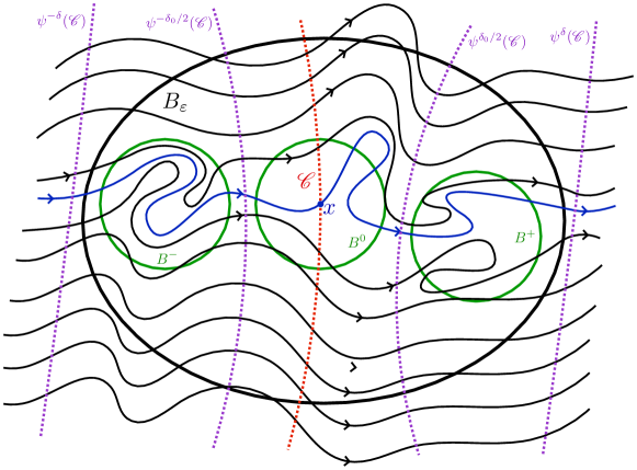
Figure 1: Sketch of the flow in ${\mathscr{U}}$ (and the subset $B_{\varepsilon}(x)\cap{\mathscr{D}}$) through the section ${\mathscr{C}}$. The time section $\sigma=\pm\delta_{0}/2$ separate the balls $B^{0}$ and $B^{\pm}$. We note that the section ${\mathscr{C}}$ (and its forward and backward translates in time) are not (necessarily) curves.

Remark 4.6.

In fact, as we will see later, we need to apply a variant of the above lemma to closed, forward invariant subsets of the form

$$\operatorname{cl}(\gamma(w)\cup\{\phi^{\sigma}(u),\sigma\geq\sigma_{*}\}),$$

where $u\in X,w\in\omega(u),\sigma_{*}\in{\mathbb{R}}.$ On $\operatorname{cl}(\gamma(w)\cup\{\phi^{\sigma}(u),\sigma\geq\sigma_{*}\})$ we have a commuting diagram similar to (4.4). In order to have a bi-directional local flow, we define the slightly smaller set

$${\mathscr{V}}:=\pi\operatorname{cl}(\gamma(w)\cup\{\phi^{\sigma}(u),\sigma\geq\sigma_{*}+2\delta\}),$$ (4.5)

for $\delta>0$ small. Then, if $x\in{\mathscr{V}}$ is not an equilibrium for $\psi^{\sigma},$ Lemma 4.5 continues to hold with ${\mathscr{U}}$ replaced by ${\mathscr{V}}$.

Remark 4.7.

(i) The second part of Lemma 4.5 is used to construct a set that replaces the role of the transversal. Let $y_{1}$ and $y_{2}$ be two points in ${\mathscr{C}}_{0}$. Consider the line segment $L_{0}$ connecting $y_{1}$ and $y_{2}$. Then $L_{0}\subset B^{0}$. It may happen that $L_{0}$ intersects the flow lines of $\psi^{\sigma}(y_{1,2})$ at some $\sigma\neq 0$, but this can be overcome by slightly varying $\sigma$. Indeed, let the line segment $\ell_{0}$ be a subset of $L_{0}$ with endpoints $\psi^{\sigma^{0}_{1}}(y_{1})$ and $\psi^{\sigma^{0}_{2}}(y_{2})$ for some $\sigma^{0}_{1},\sigma^{0}_{2}\in(-\delta_{0}/2,\delta_{0}/2)$, such that $\ell_{0}$ does not intersect the flow lines $\psi^{\sigma}(y_{1})$ and $\psi^{\sigma}(y_{2})$ at any other $\sigma\in[-\delta,\delta]$. We still have $\ell_{0}\subset B^{0}$, see Figure 2.

We repeat this construction in the balls $B^{-}$ and $B^{+}$ to obtain line segments $\ell_{-}$ and $\ell_{+}$, respectively, with one end point on each flow line and no other intersections with the flow lines.

Then we obtain three Jordan curves

$${\mathscr{J}}_{0} =\{\psi^{\sigma}(y_{1}):\sigma^{-}_{1}\leq\sigma\leq\sigma^{+}_{1}\}\cup\{\psi^{\sigma}(y_{2}):\sigma^{-}_{2}\leq\sigma\leq\sigma^{+}_{2}\}\cup\ell_{-}\cup\ell_{+},$$

$${\mathscr{J}}_{-} =\{\psi^{\sigma}(y_{1}):\sigma^{-}_{1}\leq\sigma\leq\sigma^{0}_{1}\}\cup\{\psi^{\sigma}(y_{2}):\sigma^{-}_{2}\leq\sigma\leq\sigma^{0}_{2}\}\cup\ell_{-}\cup\ell_{0},$$

$${\mathscr{J}}_{+} =\{\psi^{\sigma}(y_{1}):\sigma^{0}_{1}\leq\sigma\leq\sigma^{+}_{1}\}\cup\{\psi^{\sigma}(y_{2}):\sigma^{0}_{2}\leq\sigma\leq\sigma^{+}_{2}\}\cup\ell_{0}\cup\ell_{+}.$$

in $B_{\varepsilon}(x)$, see Figure 2. We denote the interior of ${\mathscr{J}}_{j}$ by $J_{j}$, and its exterior by $J_{j}^{*}$, $j\in\{-,0,+\}$. Clearly, $J_{\pm}\subset J_{0}$ and $J_{-}\cap J_{+}=\varnothing$.

     

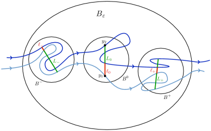
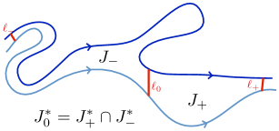
Figure 2: On the left an illustration of the construction of $\ell_{0}$ and $\ell_{\pm}$. On the right a sketch of the interiors $J_{0}$ and $J_{\pm}$ of the Jordan curves ${\mathscr{J}}_{0}$ and ${\mathscr{J}}_{\pm}$ (as well as their exteriors $J_{0}^{*}$ and $J_{\pm}^{*}$). Note that $J_{0}=\operatorname{int}(\overline{J_{-}\cup J_{+}})$.

(ii) By Lemma 4.5 any flow line in $J_{0}$ must leave $J_{0}$ in forward and backward time. By flow invariance of the other boundary components, a flow line can only enter or leave $J_{0}$ through $\ell_{+}$ or $\ell_{-}$. Moreover, no flow line can (in forward time) enter $J_{0}$ through $\ell_{+}$ and then leave it through $\ell_{-}$. In this sense, the set $J_{0}$ plays the role of a transversal. Analogous statements holds for $J_{+}$ and $J_{-}$. In particular, this implies a slightly stronger statement for the flow in $J_{+}\cap J_{0}$: if a flow line is in $J_{+}$ then must leave $J_{0}$ through $\ell_{+}$. Similarly, if a flow line is in $J_{-}$ then must have entered $J_{0}$ through $\ell_{-}$.

(iii) The flow lines $\{\psi^{\sigma}(y_{1,2}):\sigma\in(\sigma^{+}_{1,2},\delta]\}$ and $\{\psi^{\sigma}(y_{1,2}):\sigma\in[-\delta,\sigma^{-}_{1,2})\}$ lie in the exterior $J_{0}^{*}$. This follows from the fact that by construction they cannot cross $\ell_{+}$ and $\ell_{-}$, respectively, and $\psi^{\pm\delta}(y_{1,2})$ all lie in $J_{0}^{*}$ by the second bullet of Lemma 4.5(i).

Proof of Proposition 3.2.

Suppose $\omega(w)$ does not contain any equilibria. Choose $\zeta\in\omega(w)$ and $\zeta^{*}\in\omega(\zeta)$, then

$$\omega(\zeta)\subseteq\omega(\omega(w))=\omega(w)\subseteq\omega(\gamma(w))=\operatorname{cl}(\gamma(w)).$$ (4.6)

Since $\zeta^{*}$ is not an equilibrium, then $\pi(\zeta^{*})$ is not an equilibrium for $\psi^{\sigma}=\pi\circ\phi^{\sigma}\circ({\rm id}\times\pi)^{-1}$ by Corollary 4.4. According to Lemma 4.5 there exists a section ${\mathscr{C}}$ for $\psi^{\sigma}$ through $x=\pi(\zeta^{*})$. Since $\zeta^{*}\in\omega(\zeta)$ there exist times $\sigma_{n}\to\infty$ such that $\phi^{\sigma_{n}}(\zeta)\to\zeta^{*}$. By Lemma 4.5 these times can be chosen such that $\pi\circ\phi^{\sigma_{n}}(\zeta)\in{\mathscr{C}}_{0}$, as defined in Lemma 4.5(ii), for $\sigma_{n}$ sufficiently large. Moreover, $\pi\circ\phi^{\sigma}(\zeta)\not\in{\mathscr{C}}_{0}$ for $\sigma\in(\sigma_{n},\sigma_{n+1}).$ We consider two cases.

Case 1. For some $n\not=n^{\prime}$, we have $\pi\circ\phi^{\sigma_{n}}(\zeta)=\pi\circ\phi^{\sigma_{n^{\prime}}}(\zeta)$. Then, since $\pi$ is a homeomorphism on $\operatorname{cl}\bigl{(}\gamma(w)\bigr{)}$ (see Lemma 4.3) and since $\omega(\zeta)\subset\operatorname{cl}\bigl{(}\gamma(w)\bigr{)}$ (see Equation (4.6)), it follows that $\phi^{\sigma_{n}}(\zeta)=\phi^{\sigma_{n^{\prime}}}(\zeta)$, and thus $\phi^{\sigma}(\zeta)$ is a periodic orbit.

Case 2. All $\pi\circ\phi^{\sigma_{n}}(\zeta)$ are mutually distinct. Take $n$ sufficiently large so that $y_{1}\equiv\pi\circ\phi^{\sigma_{n+1}}(\zeta)$ and $y_{2}\equiv\pi\circ\phi^{\sigma_{n+1}}(\zeta)$ both lie in ${\mathscr{C}}_{0}$. Denote $\widetilde{\sigma}=\sigma_{n+1}-\sigma_{n}$, so that $y_{2}=\psi^{\widetilde{\sigma}}(y_{1})$. Apply the construction of Remark 4.7(i) to these $y_{1}$ and $y_{2}$. In addition to ${\mathscr{J}}_{0}$ we obtain two more Jordan curves

$${\mathscr{G}}_{-} =\{\psi^{\sigma}(y_{1}):\sigma^{-}_{1}\leq\sigma\leq\widetilde{\sigma}+\sigma^{-}_{2}\}\cup\ell_{-}$$

$${\mathscr{G}}_{+} =\{\psi^{\sigma}(y_{1}):\sigma^{+}_{1}\leq\sigma\leq\widetilde{\sigma}+\sigma^{+}_{2}\}\cup\ell_{+}.$$

Both curves separate ${\mathbb{R}}^{2}$ into two open sets, say $A_{\pm}^{1}$ and $A_{\pm}^{2}$, see Figure 3. Here, to fix notation, we require that $J_{0}\subset A_{+}^{1}$ and $J_{0}\subset A_{-}^{2}$ (recall that $J_{0}$ is the interior of ${\mathscr{J}}_{0}$) so that $A_{+}^{2}\cap A_{-}^{1}=\varnothing$. It follows from the property of $J_{0}$ described in Remark 4.7(ii) and flow invariance of $\{\psi^{\sigma}(y_{1}):\sigma^{-}_{1}\leq\sigma\leq\widetilde{\sigma}+\sigma^{+}_{2}\}$ that once a flow line is in $A_{+}^{2}$ it can never enter $A_{-}^{1}$ (in forward time).

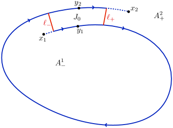
Figure 3: Sketch of the construction of $A_{+}^{2}$ and $A_{-}^{1}$. Whether $A_{-}^{1}$ is a bounded region and $A_{+}^{2}$ an unbounded one (as depicted here) or the other way around, is irrelevant for the argument.

Finally, we note that Remark 4.7(iii) implies that $x_{1}=\psi^{-\delta}(y_{1})=\pi\circ\phi^{\sigma_{n}-\delta}(\zeta)$ lies in $A_{-}^{1}$, while $x_{2}=\psi^{\delta}(y_{2})=\pi\circ\phi^{\sigma_{n+1}+\delta}(\zeta)$ lies in $A_{+}^{2}$. Now consider the orbit $\pi\circ\phi^{\sigma}(w)$. Since $\zeta\in\omega(w)$ and $\pi$ is continuous, $\pi(\zeta)$ is an $\omega$-limit point of $\pi(w)$ under $\psi^{\sigma}$. Consequently, the orbit $\pi\circ\phi^{\sigma}(w)$ keeps (in forward time) visiting arbitrarily small neighborhoods of $x_{1}\in A_{-}^{1}$ and $x_{2}\in A_{+}^{2}$. However, as argued above, once a flow line is in $A_{+}^{2}$ it can never enter $A_{-}^{1}$, which is a contradiction. ∎

Remark 4.8.

In [6, Proposition 2] the “soft version” was proved using both smoothness of the flow and fact that there exists a non-negative discrete Lyapunov function. The extension given by Proposition 3.2 makes it applicable to the Cauchy-Riemann equations, for which a ${\mathbb{Z}}$-valued Lyapunov function exists.

5 The strong version

The first subsection contains preliminary lemmas that are used to prove the strong version of the Poincaré-Bendixson Theorem. The proof of Proposition 3.3 is carried out in the second subsection. The arguments in this section resemble those in [6], but are adjusted to our setting.

5.1 Technical lemmas

Lemma 5.1.

Let $u\in X,$ then for every $w\in\omega(u)$ there exists an integer $k(w)$ such that

$$W(w^{1},w^{2})=k(w),$$

for all $w^{1},w^{2}\in\operatorname{cl}\bigl{(}\gamma(w)\bigr{)}$, with $w^{1}\not=w^{2}.$

Proof (cf. [6], Lemma 3.1)..

Since we consider two distinct $w^{1},w^{2}\in\operatorname{cl}\bigl{(}\gamma(w)\bigr{)}$, we may exclude the case that $w$ is an equilibrium. We therefore distinguish two cases: (i) $\gamma(w)$ is a periodic orbit, or (ii) $\sigma\mapsto\phi^{\sigma}(w)$ is injective. Lemma 4.2 implies that $(w^{1},w^{2})\not\in\Sigma$, and therefore $(w^{1},w^{2})\mapsto W(w^{1},w^{2})$ is a continuous ${\mathbb{Z}}$-valued function on $\bigl{(}\operatorname{cl}(\gamma(w))\times\operatorname{cl}(\gamma(w))\bigr{)}\setminus\Delta$.

(i) If $\gamma(w)$ is a periodic orbit, then, $\operatorname{cl}(\gamma(w))=\gamma(w)$, which is homeomorphic to $S^{1},$ and $\gamma(w)\times\gamma(w)$ is thus homeomorphic to the 2-torus $\mathbb{T}^{2}$. Therefore $(w^{1},w^{2})\mapsto W(w^{1},w^{2})$ induces a continuous ${\mathbb{Z}}$-valued function on $\mathbb{T}^{2}\setminus S^{1}$. Since the latter is connected, it follows that $W$ is constant on $\bigl{(}\gamma(w)\times\gamma(w)\bigr{)}\setminus\Delta$.

(ii) If $\sigma\to\phi^{\sigma}(w)$ is injective, then $\bigl{(}\gamma(w)\times\gamma(w)\bigr{)}\setminus\Delta$ has two connected components given by $(\phi^{\sigma_{1}}(w),\phi^{\sigma_{2}}(w))$, with $\sigma_{1}>\sigma_{2}$, and $\sigma_{1}<\sigma_{2},$ respectively. Since $W$ is symmetric (Axiom (A1)) we conclude that $W$ is constant on $\bigl{(}\gamma(w)\times\gamma(w)\bigr{)}\setminus\Delta$. Note that $\bigl{(}\operatorname{cl}(\gamma(w))\times\operatorname{cl}(\gamma(w))\bigr{)}\setminus\Delta$ is the closure of $\bigl{(}\gamma(w)\times\gamma(w)\bigr{)}\setminus\Delta$ in $(X\times X)\setminus\Delta$. Since $W$ is continuous on $\bigl{(}\operatorname{cl}(\gamma(w))\times\operatorname{cl}(\gamma(w))\bigr{)}\setminus\Delta$, it is also constant, which proves the lemma. ∎

Lemma 5.2.

Assume that $u\in X$ and $w\in\omega(u).$ Let $k(w)$ be defined as in Lemma 5.1. If $\alpha(w)\cap\omega(w)=\varnothing$, then there exists a $\sigma_{*}\geq 0$, such that

$$W(u^{1},w^{1})=k(w)$$ (5.1)

for every $u^{1}\in\operatorname{cl}\{\phi^{\sigma}(u),\sigma\geq\sigma_{*}\}$ and every $w^{1}\in\operatorname{cl}(\gamma(w))$, such that $u^{1}\not=w^{1}.$ In particular, if $\pi(u^{1})=\pi(w^{1})$ for some $u^{1}\in\operatorname{cl}\{\phi^{\sigma}(u),\sigma\geq\sigma_{*}\}$ and $w^{1}\in\operatorname{cl}(\gamma(w))$, then $u^{1}=w^{1}.$ Hence

$$\pi\circ\phi^{\sigma}(u)\not\in\pi\operatorname{cl}(\gamma(w))\ \ \text{for all }\sigma\geq\sigma_{*}.$$ (5.2)

Proof (cf. [6], Lemma 3.2)..

We start by observing that it is enough to prove that (5.1) holds for $u^{1}\in\phi^{\sigma}(u),\sigma\geq\sigma_{*}.$ Then by continuity of $W,$ the statement follows for all $u^{1}\in\operatorname{cl}\{\phi^{\sigma}(u),\sigma\geq\sigma_{*}\}.$

Suppose there exist sequences $\sigma_{n}\to\infty,{w}_{n}\in\operatorname{cl}(\gamma(w)),$ with

$$\phi^{\sigma_{n}}(u)\not={w}_{n},\quad k_{n}:=W(\phi^{\sigma_{n}}(u),{w}_{n})\not=k(w).$$

We may assume, passing to a subsequence if necessary, that for all $n$ we have either $k_{n}>k(w)$ or $k_{n}<k(w).$ We will split the proof in two cases.

Case 1: $k_{n}<k(w).$ Again passing to a subsequence if necessary, we may assume that either ${w}_{n}\in\alpha(w)$ for all $n$ or else ${w}_{n}\in\operatorname{cl}(\gamma(w))\setminus\alpha(w)$ for all $n.$ Since $\alpha(w)$ and $\omega(w)$ are disjoint by assumption, it follows that $\operatorname{cl}(\gamma(w))\setminus\alpha(w)=\gamma(w)\cup\omega(w).$ Choose now $w^{1}\in\omega(w)$ in case ${w}_{n}\in\alpha(w),$ and $w^{1}\in\alpha(w)$ in case ${w}_{n}\in\gamma(w)\cup\omega(w).$ In both cases we have $w^{1}\in\omega(u),$ hence we can choose a sequence $\tilde{\sigma}_{n}$ with $\tilde{\sigma}_{n}>\sigma_{n},$ for every $n$ such that

$$w^{1}:=\lim_{n\to\infty}\phi^{\tilde{\sigma}_{n}}(u).$$

In case ${w}_{n}\in\gamma(w)\cup\omega(w)$ we may assume that $\tilde{\sigma}_{n}-\sigma_{n}$ is so large that $\phi^{\tilde{\sigma}_{n}-\sigma_{n}}({w}_{n})\in\operatorname{cl}\{\phi^{\sigma}(w),\sigma>0\}.$ For a further subsequence, we have convergence of $\phi^{\tilde{\sigma}_{n}-\sigma_{n}}({w}_{n}).$ Define

$$w^{2}:=\lim_{n\to\infty}\phi^{\tilde{\sigma}_{n}-\sigma_{n}}({w}_{n}).$$

Note that $w^{1},w^{2}\in\operatorname{cl}(\gamma(w)),$ and $w^{1}\not=w^{2}$ since $\alpha(w)\cap\omega(w)=\varnothing.$ In fact, by construction it follows that either $w^{1}\in\omega(w)$ and $w^{2}\in\alpha(w),$ or else $w^{1}\in\alpha(w)$ and $w^{2}\in\operatorname{cl}\{\gamma(w),\sigma\geq 0\}=\{\phi^{\sigma}(w),\sigma\geq 0\}\cup\omega(w).$ By Lemma 5.1 there exists $k(w)\in{\mathbb{Z}}$ such that

$$W(w^{1},w^{2})=k(w).$$

For $n$ large enough the continuity of $W$ implies

$$k_{n}<k(w) = W(w^{1},w^{2})=W(\phi^{\tilde{\sigma}_{n}}(u),\phi^{\tilde{\sigma}_{n}-\sigma_{n}}({w}_{n}))$$

$$= W(\phi^{{\sigma}_{n}+(\tilde{\sigma}_{n}-\sigma_{n})}(u),\phi^{\tilde{\sigma}_{n}-\sigma_{n}}({w}^{n}))$$

$$\leq W(\phi^{{\sigma}_{n}}(u),{w}_{n})=k_{n},$$

which is a contradiction.

The final assertion (5.2) follows from the following observation. Suppose, by contradiction, that there exist a $u^{1}=\phi^{\sigma_{1}}(u),$ for some $\sigma_{1}\geq\sigma_{*}$ and $w^{1}\in\operatorname{cl}(\gamma(w)),$ such that $\pi(u^{1})=\pi(w^{1}).$ By what we have just proved, we then have $u^{1}=w^{1}.$ Since $w^{1}\in\operatorname{cl}(\gamma(w))$ and, by assumption, the sets $\alpha(w),$ $\gamma(w)$ and $\omega(w)$ are disjoint, there are only three different possibilities.

1. $w^{1}\in\omega(w).$ Then $\phi^{\sigma_{1}}(u)\in\omega(w).$ By invariance $\omega(u)\subseteq\omega(\omega(w))=\omega(w).$ Since $\alpha(w)\subseteq\omega(u)\subseteq\omega(w),$ this contradicts $\alpha(w)\cap\omega(w)=\varnothing.$

2. $w^{1}\in\alpha(w).$ Then $\phi^{\sigma_{1}}(u)\in\alpha(w).$ By invariance $\omega(u)\subseteq\omega(\alpha(w))=\alpha(w).$ Since $\omega(w)\subseteq\omega(u)\subseteq\alpha(w),$ this contradicts $\alpha(w)\cap\omega(w)=\varnothing.$

3. $w^{1}\in\gamma(w).$ Then $\phi^{\sigma_{1}}(u)\in\gamma(w).$ By invariance $\omega(u)=\omega(w).$ But $\alpha(w)\subseteq\omega(u)=\omega(w),$ again contradicting $\alpha(w)\cap\omega(w)=\varnothing.$

Case 2: $k_{n}>k(w).$ This case is analogous to the previous one. It is enough to exchange the roles of $\alpha(w)$ and $\omega(w).$ See [6, Lemma 3.2] for further details. ∎

Remark 5.3.

Lemma 5.2 implies that the commutative diagram (4.4) extends from $\operatorname{cl}(\gamma(w))$ to $\operatorname{cl}(\gamma(w)\cup\{\phi^{\sigma}(u),\sigma\geq\sigma_{*}\}),$ if $\alpha(w)\cap\omega(w)=\varnothing.$ Additionally, by Remark 4.6, the assertions of Lemma 4.5 hold for every $x\in{\mathscr{V}}$ (defined in (4.5)) that is not an equilibrium.

Lemma 5.4.

Let $u\in X$ and let $\gamma_{1}$ and $\gamma_{2}$ be (not necessarily distinct) stationary or periodic orbits in $\omega(u)$. Then, there exists a $k=k(\gamma_{1},\gamma_{2}),k\in{\mathbb{Z}}$, such that

$$W(p^{1},p^{2})=k,$$ (5.3)

for every $p^{j}\in\gamma_{j},p^{1}\not=p^{2}.$ In particular, the projections of disjoint periodic orbits are disjoint.

Proof (cf. [6], Lemma 3.3)..

We consider the case where $\gamma_{1}$ and $\gamma_{2}$ are both periodic, the others are analogous or even simpler. We first claim that $W(p^{1},p^{2})$ is defined for every $p^{1}\in\gamma^{1}$ and every $p^{2}\in\gamma^{2}$ with $p^{1}\not=p^{2}.$ Suppose, by contradiction, that there exist $p^{1}\in\gamma^{1}$ and $p^{2}\in\gamma^{2}$ with $p^{1}\not=p^{2}$ such that $(p^{1},p^{2})\in\Sigma\setminus\Delta.$ Then, by Axiom (A4) and (A5) there exists an ${\varepsilon}_{0}>0,$ such that $(\phi^{\sigma}(p^{1}),\phi^{\sigma}(p^{2}))\not\in\Sigma$ for every $\sigma\in(-{\varepsilon}_{0},{\varepsilon}_{0})\setminus\{0\}$ and

$$W(\phi^{\sigma^{\prime}}(p^{1}),\phi^{\sigma^{\prime}}(p^{2}))<W(\phi^{\sigma}(p^{1}),\phi^{\sigma}(p^{2})),$$ (5.4)

for $\sigma^{\prime}\in(0,{\varepsilon}_{0})$ and $\sigma\in(-{\varepsilon}_{0},0).$ Set $\sigma^{\prime}=\tfrac{{\varepsilon}_{0}}{2}$ and $\sigma=-\tfrac{{\varepsilon}_{0}}{2}.$ By continuity of $W$ there exists an $\eta\in(0,\tfrac{{\varepsilon}_{0}}{2})$ such that $W$ is constant on the set

$$\mathcal{U}=\left\{(\phi^{\sigma_{1}}(p^{1}),\phi^{\sigma_{2}}(p^{2}))\ |\ -\tfrac{{\varepsilon}_{0}}{2}-\eta<\sigma_{1},\sigma_{2}<\tfrac{{\varepsilon}_{0}}{2}+\eta\right\}.$$

By periodicity of $\gamma^{1}$ and $\gamma^{2}$ there is a $\sigma_{3}>{\varepsilon}_{0}$ such that $(\phi^{\sigma_{3}}(p^{1}),\phi^{\sigma_{3}}(p^{2}))\in\mathcal{U}$ (both in the periodic and the quasi-periodic case). Now, by (5.4)

$$W(\phi^{{\varepsilon}_{0}/2}(p^{1}),\phi^{{\varepsilon}_{0}/2}(p^{2}))<W(\phi^{-{\varepsilon}_{0}/2}(p^{1}),\phi^{-{\varepsilon}_{0}/2}(p^{2}))=W(\phi^{\sigma_{3}}(p^{1}),\phi^{\sigma_{3}}(p^{2})).$$

Since $\sigma_{3}>\tfrac{{\varepsilon}_{0}}{2},$ this contradicts Lemma 4.1. Hence $(p^{1},p^{2})\not\in\Sigma$ and $W(p^{1},p^{2})$ is well defined for every $p^{1}\in\gamma^{1}$ and every $p^{2}\in\gamma^{2},$ with $p^{1}\not=p^{2}.$

This implies, by continuity of $W$, that the map

$$(p^{1},p^{2})\to W(p^{1},p^{2})$$

is locally constant on

$$\{(p^{1},p^{2})\in\gamma_{1}\times\gamma_{2}\ |\ p^{1}\not=p^{2}\}.$$

This set is connected, which proves (5.3). ∎

Lemma 5.5.

Let $u\in X$ and $e\in E.$ For every $w\in\omega(u)$ with $w\not=e$ it holds $(w,e)\not\in\Sigma.$ If, furthermore, $e\not=\omega(u)$ then there exists a $\bar{\sigma}\in{\mathbb{R}}$ such that the map $\sigma\mapsto W(\phi^{\sigma}(u),e)$ is constant for $\sigma>\bar{\sigma}.$

Proof.

The arguments in this proof resemble those in the proof of Lemma 4.2. We repeat the argument. Let $w\in\omega(u).$ Since $w\not=e,$ we can assume that $(w,e)\not\in\Delta.$ Suppose, by contradiction, that $(w,e)\in\Sigma\setminus\Delta,$ then by Axioms (A4) and (A5), there exists an ${\varepsilon}_{0}>0$ such that $(\phi^{\sigma}(w),e)\not\in\Sigma,$ for all $\sigma\in(-{\varepsilon}_{0},{\varepsilon}_{0})\setminus\{0\}$ and

$$W(\phi^{\sigma}(w),e)>W(\phi^{\sigma^{\prime}}(w),e),$$

for all $\sigma\in(-{\varepsilon}_{0},0)$ and all $\sigma^{\prime}\in(0,{\varepsilon}_{0}).$ Set $\sigma=-{\varepsilon}$ and $\sigma^{\prime}={\varepsilon},$ with $0<{\varepsilon}<{\varepsilon}_{0}.$ Then we have

$$W(\phi^{-{\varepsilon}}(w),e)>W(\phi^{{\varepsilon}}(w),e).$$ (5.5)

By definition of the $\omega$-limit set and the invariance $\omega$, there exists a sequence $\sigma_{n}\to\infty,$ as $n\to\infty$ such that

$$\phi^{\sigma_{n}\pm{\varepsilon}}(u)\to\phi^{\pm{\varepsilon}}(w).$$ (5.6)

Since $\sigma_{n}$ is divergent we assume that

$$\sigma_{n+1}>\sigma_{n}+2{\varepsilon},\quad\text{for all }n\in{\mathbb{N}}.$$ (5.7)

Inequality (5.5), convergence in (5.6) and Lemma 4.1 imply, for $\sigma_{n}\to\infty,$ that

$$\begin{array}[]{ccl}W(\phi^{\sigma_{n}+{\varepsilon}}(u),e)&=&W(\phi^{+{\varepsilon}}(w),e)\\ &<&W(\phi^{-{\varepsilon}}(w),e)\\ &=&W(\phi^{\sigma_{n}-{\varepsilon}}(u),e).\end{array}$$

Combining the latter with (5.7) and the fact that $W$ is non-increasing, we obtain

$$W(\phi^{\sigma_{n+1}-{\varepsilon}}(u),e)<W(\phi^{\sigma_{n}-{\varepsilon}}(u),e),$$

for all $n.$ From this, we deduce that $\sigma\mapsto W(\phi^{\sigma}(u),e)$ has infinitely many jumps and therefore

$$W(\phi^{\sigma}(u),e)\to-\infty\quad\text{as}\quad\sigma\to\infty.$$

On the other hand, continuity of $W$ and (5.6) imply, for $\sigma_{n}\to\infty,$ that

$$W(\phi^{\sigma_{n}+{\varepsilon}}(u),e)=W(\phi^{{\varepsilon}}(w),e)>-\infty,$$

which is a contradiction.

To prove the final assertion, suppose, by contradiction, that such a $\bar{\sigma}$ does not exist. Then there exists a sequence $\sigma_{n}\to\infty$ such that $(\phi^{\sigma_{n}}(u),e)\in\Sigma.$ Now choose a $w\in\omega(u)\setminus\{e\}\not=\varnothing.$ There exists a sequence $\tilde{\sigma}_{n}\to\infty$ such that $\phi^{\tilde{\sigma}_{n}}(u)\to w.$ By the first part of the lemma, $W(w,e)\in{\mathbb{Z}}.$ We may choose $\tilde{\sigma}_{n}>\sigma_{n}$ without loss of generality. By continuity of $W$ and axiom (A5) it follows that

$$W(w,e)=\lim_{n\to\infty}W(\phi^{\tilde{\sigma}_{n}}(u),e)=-\infty,$$

a contradiction. ∎

Lemma 5.6.

Let $u$ be in $X.$ There exists an integer $k_{0}\in{\mathbb{Z}}$ such that

$$W(w,e)=k_{0}$$ (5.8)

for every $w\in\omega(u),$ and for every equilibrium $e\in\omega(u)$ such that $w\not=e.$

Proof.

Fix $e\in E\cap\omega(u).$ Let $w\in\omega(u)\setminus\{e\}.$ According to Lemma 5.5, $W(w,e)$ is well-defined. Since $\phi^{\sigma_{n}}(u)\to w$ for some $\sigma_{n}\to\infty,$

$$W(w,e) = \lim_{n\to\infty}W(\phi^{\sigma_{n}}(u),e)$$

$$= \lim_{\sigma\to\infty}W(\phi^{\sigma}(u),e)=k_{e},$$

where the second limit exists by Lemma 5.5. Since the above statement holds for any $w\in\omega(u)\setminus\{e\},$ this implies that $W(w,e)$ is independent of $w\in\omega(u)\setminus\{e\}.$

We still need to show that $W(w,e)$ is independent of $e\in E\cap\omega(u).$ Therefore let $e,\tilde{e}\in E\cap\omega(u),e\not=\tilde{e}.$ Then, by Axiom (A1), by the fact that $e,\tilde{e}\in\omega(u),$ and by Lemma 5.5 it holds that

$$k_{e}=W(w,e)=W(\tilde{e},{e})=W(e,\tilde{e})=W(w,\tilde{e})=k_{\tilde{e}}.$$

This shows (5.8) and concludes the proof. ∎

5.2 Proof of the strong version

In this subsection we prove Propositions 3.3 and 3.4, which completes the proof of Theorem 3.1. Theorem 1.2 follows as a consequence of Proposition 5.7.

Proof of Proposition 3.3.

Let $u\in X$ and $w\in\omega(u)$. Suppose, by contradiction, that there is a non-equilibrium $w^{*}\in\omega(w)$ and that $\gamma(w)$ is not periodic. Lemma 4.3 implies that $\pi\circ\phi^{\sigma}$ is a planar flow on the set $\omega(w)\subseteq\operatorname{cl}(\gamma(w)).$ By Corollary 4.4 the point $\pi(w^{*})$ is not an equilibrium for $\pi\circ\phi^{\sigma}.$ According to Lemma 4.5 there exist a section ${\mathscr{C}}$ through $\pi(w^{*})$. Consider first $\pi\circ\phi^{\sigma}(w)$ and recall that by Lemma 4.3 the map $\sigma\to\pi\circ\phi^{\sigma}(w)$ is one-to-one since $\gamma(w)$ is not periodic. Let $\sigma_{n}\to\infty$ denote those positive times for which $\pi\circ\phi^{\sigma_{n}}(w)\in{\mathscr{C}}$. Note that $\{\pi\circ\phi^{\sigma_{n}}(w)\}_{n=1}^{\infty}$ are all distinct and for $n$ sufficiently large $y_{1}=\pi\circ\phi^{\sigma_{n}}(w)$ and $y_{2}=\pi\circ\phi^{\sigma_{n+1}}(w)$ both lie in ${\mathscr{C}}_{0}$. Denote $\widetilde{\sigma}=\sigma_{n+1}-\sigma_{n}$, so that $y_{2}=\psi^{\widetilde{\sigma}}(y_{1})$. We apply the construction of Remark 4.7(i) to these $y_{1}$ and $y_{2}$. In addition to ${\mathscr{J}}_{0}$ and ${\mathscr{J}}_{\pm}$ we obtain three more Jordan curves (the first two are the same as in the proof of Proposition 3.2)

$${\mathscr{G}}_{-} =\{\psi^{\sigma}(y_{1}):\sigma^{-}_{1}\leq\sigma\leq\widetilde{\sigma}+\sigma^{-}_{2}\}\cup\ell_{-}$$

$${\mathscr{G}}_{+} =\{\psi^{\sigma}(y_{1}):\sigma^{+}_{1}\leq\sigma\leq\widetilde{\sigma}+\sigma^{+}_{2}\}\cup\ell_{+}$$

$${\mathscr{G}}_{0} =\{\psi^{\sigma}(y_{1}):\sigma^{0}_{1}\leq\sigma\leq\widetilde{\sigma}+\sigma^{0}_{2}\}\cup\ell_{0}.$$

These three curves separate ${\mathbb{R}}^{2}$ into two open sets, say $A_{j}^{1}$ and $A_{j}^{2}$, with $j\in\{-,0,+\}$. To fix notation, we require that $J_{0}\subset A_{+}^{1}$ and $J_{0}\subset A_{-}^{2}$ and $J_{+}\subset A_{+}^{2}$, see Figure 4. In particular, this implies that $A_{+}^{2}\subset A_{0}^{2}\subset A_{-}^{2}$ and $A_{+}^{2}\cap A_{-}^{1}=\varnothing$, as well as $A_{+}^{2}\cap A_{0}^{1}=\varnothing$ and $A_{-}^{1}\cap A_{0}^{2}=\varnothing$. It follows from the properties of $J_{0}$ and $J_{\pm}$ described in Remark 4.7(ii) and invariance of $\{\psi^{\sigma}(y_{1}):\sigma^{-}_{1}\leq\sigma\leq\widetilde{\sigma}+\sigma^{+}_{2}\}$ that in forward time once a flow line is in $A_{+}^{2}$ it can never enter $A_{0}^{1}$, while in backward time once a flow line is in $A_{-}^{1}$ it can never enter $A_{0}^{2}$. We note that Remark 4.7(iii) implies that $x_{1}=\pi\circ\phi^{\sigma_{n}-\delta}(w)$ lies in $A_{-}^{1}$, while $x_{2}=\pi\circ\phi^{\sigma_{n+1}+\delta}(w)$ lies in $A_{+}^{2}$. Therefore, $\pi\omega(w)\subset A_{0}^{2}$, while $\pi\alpha(w)\subset A_{0}^{1}$, cf.  Figure 4. Hence $\pi\omega(w)\cap\pi\alpha(w)=\varnothing$. We infer from Lemma 4.3 that $\alpha(w)\cap\omega(w)=\varnothing$.

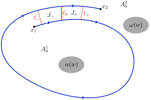
Figure 4: Sketch of the construction of $A_{\pm}^{0}$. Note that $J_{+}=A_{-}^{2}\cap A_{0}^{2}$ and $J_{-}=A_{+}^{1}\cap A_{0}^{1}$.

Next we consider the orbit of $u$. The assumptions of Lemma 5.2 are satisfied and hence there exists a time $\sigma_{*}$, such that the curve $\{\pi\circ\phi^{\sigma}(u):\sigma\geq\sigma_{*}\}$ cannot cross the curve $\pi\circ\phi^{\sigma}(w)$. Furthermore, it follows from Remarks 4.6 and 5.3 and the above construction, that once the flow line $\pi\circ\phi^{\sigma}(u)$ is in $A_{+}^{2}$ it can never enter $A_{0}^{1}$ (in forward time). Moreover, by Remark 4.7(ii), once a flow line is in $A_{0}^{2}$ then it must enter $A_{+}^{2}$ in forward time, after which it can no longer enter $A_{0}^{1}$. On the other hand, since both $\omega(w)$ and $\alpha(w)$ are contained in $\omega(u)$, the forward orbit $\pi\circ\phi^{\sigma}(u)$ will have $\omega$-limit points when $\sigma\to\infty$ in both $\pi\alpha(w)\subset A_{0}^{1}$ and $\pi\omega(w)\subset A_{0}^{2}$. This is a contradiction. ∎

Proof of Proposition 3.4 (cf. [6], Proposition 2)..

Suppose that $\omega(u)$ contains a periodic orbit $\gamma(p)$ as a strict subset. Let $V\subseteq X$ be a closed tubular neighborhood of $\gamma(p).$ Choose $V$ small enough such that it does not contain equilibria and such that $\omega(u)$ still has elements outside $V.$ Since there are accumulation points (for $\phi^{\sigma}(u)$ when $\sigma$ goes to infinity) both inside and outside $V,$ then $\phi^{\sigma}(u)$ must enter and leave $V$ infinitely often. Let $\sigma_{n}\to\infty$ be a sequence such that

$$p=\lim_{n\to\infty}\phi^{\sigma_{n}}(u)$$

and such that $\phi^{\sigma}(u)$ leaves $V$ between any two consecutive times $\sigma_{n}.$ Let $I_{n}:=[\sigma_{n}-\alpha_{n},\sigma_{n}+\beta_{n}]$ be the maximal time interval containing $\sigma_{n}$ such that

$$\phi^{\sigma}(u)\in V\ \ \ \text{for all }\sigma\in I_{n}.$$

Since $\partial V$ is closed, we may assume convergence (passing to a subsequence, if necessary) of $\phi^{\sigma_{n}-\alpha_{n}}(u).$ Note that $\sigma_{n-1}<\sigma_{n}-\alpha_{n}$ thus $\sigma_{n}-\alpha_{n}\to\infty.$ Let

$$q:=\lim_{n\to\infty}\phi^{\sigma_{n}-\alpha_{n}}(u)\in\omega(u),$$

and $q\in\partial V.$ Moreover we may assume that $\alpha_{n}+\beta_{n}\to\infty$ (at least for a subsequence) since $\omega(u)$ contains a periodic orbit in the interior of $V.$ We have thus

$$\omega(q)\subseteq\operatorname{cl}(\phi^{\sigma}(q))\subseteq V,\ \ \sigma>0.$$

From Proposition 3.3 we conclude that $\gamma(q)$ is periodic. By construction $\gamma(q)$ and $\gamma(p)$ are distinct and $\gamma(q)$ is contained in $V.$ By continuity of the flow and the projection $\pi$ and by the compactness of $V$, the sets $\pi\gamma(p)$ and $\pi\gamma(q)$ are close in the Hausdorff metric (of compact subsets of ${\mathbb{R}}^{2}$) provided that we take the tubular neighborhood $V$ sufficiently small. From this it follows that $\pi\gamma(q)$ and $\pi\gamma(p)$ are nested closed curves. Reducing $V$ to separate $\gamma(p)$ from $\gamma(q),$ a periodic solution $\gamma(r)$ can be constructed in the same way. Note once more that $\pi\gamma(q),\pi\gamma(p)$ and $\pi\gamma(r)$ are nested closed curves. Applying Lemma 5.4 to the trajectories $\gamma(p)$ and $\gamma(q)$ we conclude that there exists a $k\in{\mathbb{Z}}$ such that

$$W(p^{1},q^{1})=k,$$

for all $p^{1}\in\gamma(p)$ and $q^{1}\in\gamma(q).$ By continuity of $W$ (Axiom (A1)) this implies that

$$W(p^{1},\phi^{\sigma_{n}-\alpha_{n}}(u))=k,$$

for all $p^{1}\in\gamma(p)$ when $n$ is big enough, since $\phi^{\sigma_{n}-\alpha_{n}}(u)\to q\in\gamma(q).$ By Assumption (A5) we get $\pi\circ\phi^{\sigma}(u)\not\in\pi\gamma(p)$ for every $\sigma$ in the open interval with endpoints $\sigma_{n}-\alpha_{n},\sigma_{m}-\alpha_{m},$ provided $n,m$ are chosen large enough. Since $\sigma_{m}-\alpha_{m}\to\infty,$ as $m\to\infty,$ it follows that $\pi\circ\phi^{\sigma}(u)\not\in\pi\gamma(p),$ for any $\sigma$ large enough. In an analogous manner we can prove that, for $\sigma$ large enough, the curve $\pi\circ\phi^{\sigma}(u)$ can never intersect $\pi\gamma(q)$ and $\pi{\gamma}(r),$ but this is a contradiction since $\pi\circ\phi^{\sigma}(u)$ has $\omega$-limit points as $\sigma\to\infty$ in the three nested curves $\pi{\gamma}(p),\pi{\gamma}(q),\pi{\gamma}(r).$ ∎

Proposition 5.7.

Let $u\in X$. Then,

$$\pi:\omega(u)\to\pi(\omega(u))$$

is a homeomorphism onto its image. Hence $\pi\circ\phi^{\sigma}$ is a flow on $\pi(\omega(u)).$

Proof (cf. [6], Theorem 2)..

By Axiom (A5) it is enough to show that there exists a $k_{0}\in{\mathbb{Z}}$ such that

$$W(w^{1},w^{2})=k_{0},$$ (5.9)

for all $w^{1},w^{2}\in\omega(u),w^{1}\not=w^{2}.$ We now apply Theorem 3.1 (Poincaré-Bendixson). If $\omega(u)$ consists of a single periodic orbit, then (5.9) holds by Lemma 5.4. We may therefore assume for the remainder of the proof that for every $w\in\omega(u)$ we have $\alpha(w),\omega(w)\subseteq E.$ If either $w^{1}$ or $w^{2}$ is an equilibrium then (5.9) holds with $k_{0}$ defined in Lemma 5.6. We may therefore assume that $w^{1}\not\in E.$ Suppose now, by contradiction, that there exist $(w^{1},w^{2})\in\Sigma\setminus\Delta.$ By Axioms (A4) and (A5) there exists an ${\varepsilon}_{0}>0$ such that $\bigl{(}\phi^{\sigma}(w^{1}),\phi^{\sigma}(w^{2})\bigr{)}\not\in\Sigma$, for all $\sigma\in(-{\varepsilon}_{0},{\varepsilon}_{0})\setminus\{0\}$ and

$$W(\phi^{\sigma^{\prime}}(w^{1}),\phi^{\sigma^{\prime}}(w^{2}))<W(\phi^{\sigma}(w^{1}),\phi^{\sigma}(w^{2})),$$

for all $\sigma\in(-{\varepsilon}_{0},0)$ and all $\sigma^{\prime}\in(0,{\varepsilon}_{0})$. Set $\sigma=-{\varepsilon}$ and $\sigma^{\prime}={\varepsilon}$, with $0<{\varepsilon}<{\varepsilon}_{0}$. Since $w^{1}\in\omega(u),$ there exists $\sigma_{n}\to\infty$ such that

$$w^{1}=\lim_{n\to\infty}\phi^{\sigma_{n}}(u),$$

and

$$0<\sigma_{n+1}-\sigma_{n}\to\infty,\ \ \text{as}\ \ n\to\infty.$$

Define $\hat{\sigma}_{n}:=(\sigma_{n+1}-\sigma_{n})\to\infty$. Then, passing to a subsequence if necessary, the limits

$$e:=\lim_{n\to\infty}\phi^{-\hat{\sigma}_{n}}(\phi^{-{\varepsilon}}(w^{2}))\quad\text{and}\quad\tilde{e}:=\lim_{n\to\infty}\phi^{\hat{\sigma}_{n}}(\phi^{{\varepsilon}}(w^{2}))$$

exist, and $e,\tilde{e}\in E,$ since $\alpha(w^{2})\subseteq E$ and $\omega(w^{2})\subseteq E.$ By Axiom (A1), Lemma 4.1, Lemma 5.6 and the fact that $w^{1}\not\in E$ we infer that, for $n$ sufficiently large (slightly shifting ${\varepsilon}$ if necessary to make $W$ well-defined for all relevant pairs)

$$\begin{array}[]{lll}W(\phi^{{\varepsilon}}(w^{1}),\phi^{{\varepsilon}}(w^{2}))&<&W(\phi^{-{\varepsilon}}(w^{1}),\phi^{-{\varepsilon}}(w^{2}))\\ &=&W(\phi^{\sigma_{n+1}-{\varepsilon}}(u),\phi^{-{\varepsilon}}(w^{2}))\\ &\leq&W(\phi^{\sigma_{n+1}-\hat{\sigma}_{n}-{\varepsilon}}(u),\phi^{-\hat{\sigma}_{n}-{\varepsilon}}(w^{2}))\\ &=&W(\phi^{\sigma_{n}-{\varepsilon}}(u),e)\\ &=&W(\phi^{-{\varepsilon}}(w^{1}),e)\\ &=&W(\phi^{-{\varepsilon}}(w^{1}),\tilde{e})\\ &=&W(\phi^{{\varepsilon}}(w^{1}),\tilde{e})\\ &=&W(\phi^{\sigma_{n+1}+{\varepsilon}}(u),\tilde{e})\\ &=&W(\phi^{\hat{\sigma}_{n}+\sigma_{n}+{\varepsilon}}(u),\phi^{\hat{\sigma}_{n}+{\varepsilon}}(w^{2}))\\ &\leq&W(\phi^{\sigma_{n}+{\varepsilon}}(u),\phi^{{\varepsilon}}(w^{2}))\\ &=&W(\phi^{{\varepsilon}}(w^{1}),\phi^{{\varepsilon}}(w^{2})),\end{array}$$

which is a contradiction. In the sixth and in the seventh equality we used Lemma 5.6. ∎

Since the Cauchy-Riemann Equations satisfy the Axioms (A1)-(A5) Theorem 1.2 follows from Proposition 5.7.

6 Proofs of Propositions 2.1 and 2.3

Consider the operators

$$\partial=\partial_{s}-J\partial_{t}\ \ \text{and}\ \ \overline{\partial}=\partial_{s}+J\partial_{t},$$

and recall the following regularity estimates:

Lemma 6.1.

Let $g$ be a function in $\in C^{\infty}_{c}({\mathbb{R}}\times S^{1};{\mathbb{R}}^{2}).$ For every $1<p<\infty$, there exists a constant $C_{p}>0$, such that

$$\|\nabla g\|_{L^{p}({\mathbb{R}}\times S^{1})}\leq C_{p}\|\bar{\partial}g\|_{L^{p}({\mathbb{R}}\times S^{1})}.$$ (6.1)

The same estimate holds for $\partial$ via $t\mapsto-t$.

Proof.

See [1], [5] [8], [9, appendix B]. ∎

Proof of Proposition 2.1.

For a solution $u\in X,$ we can write

$$\overline{\partial}u=-JF(t,u)=f(s,t),$$ (6.2)

where $F,$ and therefore $f$, are uniformly bounded since for every $u\in X$ we have

$$\|u\|_{L^{\infty}({\mathbb{R}}\times S^{1})}\leq 1.$$ (6.3)

Extend $f$ and $u$ via periodic extension to a function on ${\mathbb{R}}^{2}$ in the $t$-direction. By $L^{\infty}$-bound on $u$ we obtain the existence of a constant $M>0,$ such that

$$\|f\|_{L^{\infty}({\mathbb{R}}^{2})}\leq M.$$ (6.4)

Let $K,L,G$ be compact sets contained in ${\mathbb{R}}^{2}$ such that $K\Subset L\Subset G\subset\mathbb{R}^{2},$ and let ${\varepsilon}$ be positive such that ${\varepsilon}<\operatorname{dist}(L,\partial G).$ By compactness, $L$ can be covered by finitely many open balls of radius ${\varepsilon}/2:$

$$L\subset\bigcup_{i=1}^{N_{\varepsilon}}B_{{\varepsilon}/2}(x_{i}).$$

Consider a partition of unity $\{\rho_{{\varepsilon},x_{i}}\}_{i=1,\dots,N_{\varepsilon}}$ on $L$ subordinate to $\left\{B_{{\varepsilon}}(x_{i})\right\}_{i=1,\dots,N_{\varepsilon}}\!\!.$ In particular the supports of $\rho_{{\varepsilon},x_{i}}$ are contained in $B_{{\varepsilon}}(x_{i}),$ for every $i=1\dots N_{{\varepsilon}}.$ Then, for every $u,$ every small ${\varepsilon}>0$ and every $i=1\dots N_{{\varepsilon}},$ the function $v_{{\varepsilon},i}:=\rho_{{\varepsilon},x_{i}}u$ belongs to $W^{k,p}_{0}({\mathbb{R}}^{2}),$ for every $p\geq 1,$ and every $k\in{\mathbb{N}}.$ For such functions the Poincaré inequality $\|v_{{\varepsilon},i}\|_{L^{p}(B_{\varepsilon}(x_{i}))}\leq C\|\nabla v_{{\varepsilon},i}\|_{L^{p}(B_{\varepsilon}(x_{i}))}$ holds. Combining the latter with Lemma 6.1 yields (with $C$ changing from line to line)

$$\begin{array}[]{ll}\|v_{{\varepsilon},i}\|_{W^{1,p}({\mathbb{R}}^{2})}&=\|v_{{\varepsilon},i}\|_{W^{1,p}(B_{\varepsilon}(x_{i}))}\leq C\|v_{{\varepsilon},i}\|_{W^{1,p}_{0}(B_{\varepsilon}(x_{i}))}\\ &\leq C\|\overline{\partial}v_{{\varepsilon},i}\|_{L^{p}(B_{\varepsilon}(x_{i}))}\\ &\leq C\|\rho_{{\varepsilon},x_{i}}\overline{\partial}u\|_{L^{p}(B_{\varepsilon}(x_{i}))}+C\|u\overline{\partial}\rho_{{\varepsilon},x_{i}}\|_{L^{p}(B_{\varepsilon}(x_{i}))}\\ &\leq C\|\overline{\partial}u\|_{L^{p}(G)}+C\|u\|_{L^{p}(G)}.\end{array}$$ (6.5)

As $\left\{\rho_{{\varepsilon},x_{i}}\right\}_{i=1,\dots,N_{{\varepsilon}}}$ is a partition of unity it follows that

$$\|u\|_{W^{1,p}(L)}=\left|\left|\sum_{i=1}^{N_{{\varepsilon}}}v_{{\varepsilon},i}\right|\right|_{W^{1,p}(L)}\leq\sum_{i=1}^{N_{{\varepsilon}}}\|v_{{\varepsilon},i}\|_{W^{1,p}(B_{\varepsilon}(x_{i}))}.$$ (6.6)

By (6.5) and (6.6) we obtain

$$\|u\|_{W^{1,p}(L)}\leq C_{p,L,G}\left(\|\overline{\partial}u\|_{L^{p}(G)}+\|u\|_{L^{p}(G)}\right).$$ (6.7)

Combining (6.7) with (6.2), (6.3) and (6.4) yields

$$\|u\|_{W^{1,p}(L)}\leq C_{p,L,G}\left(\|f\|_{L^{p}(G)}+\|u\|_{L^{p}(G)}\right)\leq C_{p,L,G}^{1},$$ (6.8)

where the constant $C_{p,L,G}^{1}$ depends on $p,L,G$, but not on $u.$ By the compactness of the Sobolev compact embedding $W^{1,p}(L)\hookrightarrow C^{0}(L)$, cf. [2], sequences $\{u^{n}\}\subset X$ have convergent subsequences in $C^{0}_{\text{loc}}(L).$ Since the latter holds for every $L\subset{\mathbb{R}}^{2},$ the convergence is in $C^{0}_{\text{loc}}({\mathbb{R}}^{2})$ and the limit $u$ is a continuous function. It remains to show that the limit $u$ solves Equation (1.2). Consider a partition of unity of $K\Subset L,$ denoted $\{\rho_{{\varepsilon},x_{i}}\}_{i=1,\dots N_{{\varepsilon}}}$, where $0<{\varepsilon}<\operatorname{dist}(K,\partial L).$ On balls $B_{{\varepsilon}}(x_{i})$ we obtain

$$\begin{array}[]{ll}\|\rho_{{\varepsilon},x_{i}}u\|_{W^{2,p}(B_{{\varepsilon}})}&\leq C\|\rho_{{\varepsilon},x_{i}}u\|_{W^{2,p}_{0}(B_{{\varepsilon}}(x_{i}))}\leq C\|\overline{\partial}(\rho_{{\varepsilon},x_{i}}u)\|_{W^{1,p}(B_{{\varepsilon}}(x_{i}))}\\ &\leq C\displaystyle\left(\|\rho_{{\varepsilon},x_{i}}\overline{\partial}u\|_{W^{1,p}(B_{{\varepsilon}}(x_{i}))}+\|u\overline{\partial}\rho_{{\varepsilon},x_{i}}\|_{W^{1,p}(B_{{\varepsilon}}(x_{i}))}\right)\\ &\leq C\left(\|\overline{\partial}u\|_{L^{\infty}(L)}+\|\overline{\partial}u\|_{W^{1,p}(L)}+\|u\|_{L^{\infty}(L)}+\|u\|_{W^{1,p}(L)}\right).\end{array}$$

As in (6.6), using (6.2), we obtain

$$\|u\|_{W^{2,p}(K)}\leq\tilde{C}_{p,K,L,G}\left(\|f\|_{L^{\infty}(L)}+\|f\|_{W^{1,p}(L)}+\|u\|_{L^{\infty}(L)}+\|u\|_{W^{1,p}(L)}\right).$$ (6.9)

To estimate the three terms $\|f\|_{L^{\infty}(L)},$ $\|u\|_{L^{\infty}(L)}$ and $\|u\|_{W^{1,p}(L)}$ we use (6.3), (6.4), and (6.8). In order to control $\|f\|_{W^{1,p}(L)}$, differentiate the smooth vector field $F$:

$$f_{s}(s,t)=(F(t,u))_{s}=D_{t,u}X(t,u)(0,u_{s})$$

$$f_{t}(s,t)=(F(t,u))_{t}=D_{t,u}X(t,u)(1,u_{t}).$$

Both right hand sides lie in $L^{p}(L)$ and hence $Df=(f_{s},f_{t})$ is in $L^{p}(L).$ By (6.9) there exists a constant ${C}_{p,K,L,G}^{2}$ independent of $u$ such that

$$\|u\|_{W^{2,p}(K)}\leq{C}_{p,K,L,G}^{2}.$$

By taking $p>2$ the compact Sobolev embedding $W^{2,p}(K)\hookrightarrow C^{1}({K})$ implies that $u\in X.$ ∎

Proof of Proposition 2.3.

As in the proof of Lemma 4.3 if suffices to show that $\iota$ is injective. Suppose there exist $u_{1},u_{2}\in X$ such that $\iota(u_{1})=\iota(u_{2}).$ By definition of $\iota$ we have

$$u_{1}(0,\cdot)=u_{2}(0,\cdot).$$ (6.10)

Define $v(s,t):=u_{1}(s,t)-u_{2}(s,t),$ for all $(s,t)\in{\mathbb{R}}\times S^{1}.$ By (6.10) we have $v(0,t)=0$ for all $t\in S^{1}.$ By smoothness of the vector field $F$ we can write

$$F(t,u_{1})=F(t,u_{2})+R(t,u_{1},u_{2}-u_{1})(u_{2}-u_{1}),$$

where $R_{1}$ is a smooth function of its arguments. Upon substitution this gives

$$v_{s}-Jv_{t}+A(s,t)v=0,\quad v(0,t)=0\ \ \ \text{for all}\ t\in S^{1},$$ (6.11)

and $A(s,t)=R(t,u_{1}(s,t),v(s,t))$ is (at least) continuous on ${\mathbb{R}}\times S^{1}.$ Evaluating (6.11) at $t=0$ we obtain,

$$v_{s}-Jv_{t}+A(s,t)v=0,\quad v(0,0)=0$$ (6.12)

Introducing complex coordinates $z:=s+it,$ (6.12) becomes

$$\partial v+A(z)v=0,\quad v(0)=0,$$ (6.13)

where the operator $\partial:=\partial_{s}-i\partial_{t}$ is the standard anti-holomorphic derivative. We used the identification between the complex structure $J$ in ${\mathbb{R}}^{2}$ and $i$ in $\mathbb{C}.$ Multiplying (6.13) by $e^{\int_{0}^{z}A(\zeta)d\zeta}$ and defining

$$w(z):=e^{\int_{0}^{z}A(\zeta)d\zeta}v(z),$$

gives

$$\partial w=0,\quad w(0)=0.$$

which implies that $w$ is analytic. The latter yields that either $0$ is an isolated zero for $w$, or there exists a $\delta>0,$ such that $w(z)=0,$ on $U_{\delta}:=\{z\in\mathbb{C}:|z|\leq\delta\}.$ By (6.11) we conclude that 0 cannot be an isolated zero for $w$, hence $w\equiv 0$ in $U_{\delta}:=\{z\in\mathbb{C}:|z|\leq\delta\}.$ Repeating these arguments we obtain that $w(s,t)=0$ for all $(s,t)\in{\mathbb{R}}\times S^{1}$ and hence $v\equiv 0.$ This implies $u_{1}=u_{2},$ which concludes the proof.∎

Remark 6.2.

The same proof can be carried out in case $J$ is a smooth map ${\mathbb{R}}\times S^{1}\to\operatorname{Sp}(2,{\mathbb{R}})$ such that $J^{2}=-\operatorname{Id}$. In this case one can prove that the equation $u_{s}-J(s,t)(u_{t}-F(t,u))=0$ can be transformed into (1.2) using [8, Theorem 12, Appendix A.6].

References

- [1] A. Abbondandolo and M. Schwarz, Floer homology of cotangent bundles and the loop product, Geom. Topol. 14 (2010), no. 3, 1569–1722.
- [2] R. A. Adams, Sobolev spaces, Academic Press, 1975.
- [3] G. Aranson, S. Belitsky and E. Zhuzhoma, Introduction to the qualitative theory of dynamical systems on surfaces, Math. Monogr., vol. 153, AMS, 1996.
- [4] K. Ciesielski, The Poincaré-Bendixson theorems for two-dimensional semiflows, Topological Methods in Nonlinear Analysis 3 (1994), 163–178.
- [5] A. Douglis and L. Niremberg, Interior estimates for elliptic systems of partial differential equations, Comm. Pure Appl. Math. 8 (1955), 503–538.
- [6] B. Fiedler and J. Mallet-Paret, A Poincaré-Bendixson Theorem for Scalar Reaction Diffusion Equations, Arch. Rat. Mech. and Anal. 107 (1989), no. 4, 325–345.
- [7] O. Hájek, Dynamical Systems in the Plane, Academic Press, 1968.
- [8] H. Hofer and Zehnder E., Symplectic invariants and Hamiltonian dynamics, Birkäuser, 1994.
- [9] D. McDuff and D. Salamon, J-holomorphic curves and symplectic topology, AMS, 2004.
- [10] J. R. Munkres, Topology, Prentice Hall, 2000.
- [11] J. B. van den Berg, R. Ghrist, R. C. Vandervorst, and W. Wójcik, Braid Floer homology, J. Differential Equations 259 (2015), no. 5, 1663–1721. MR 3349416