Node-to-segment and node-to-surface interface finite elements for fracture mechanics

Abstract

The topologies of existing interface elements used to discretize cohesive cracks are such that they can be used to compute the relative displacements (displacement discontinuities) of two opposing segments (in 2D) or of two opposing facets (in 3D) belonging to the opposite crack faces and enforce the cohesive traction-separation relation. In the present work we propose a novel type of interface element for fracture mechanics sharing some analogies with the node-to-segment (in 2D) and with the node-to-surface (in 3D) contact elements. The displacement gap of a node belonging to the finite element discretization of one crack face with respect to its projected point on the opposite face is used to determine the cohesive tractions, the residual vector and its consistent linearization for an implicit solution scheme. The following advantages with respect to classical interface finite elements are demonstrated: $(i)$ non-matching finite element discretizations of the opposite crack faces is possible; $(ii)$ easy modelling of cohesive cracks with non-propagating crack tips; $(iii)$ the internal rotational equilibrium of the interface element is assured. Detailed examples are provided to show the usefulness of the proposed approach in nonlinear fracture mechanics problems.

Notice: this is the authors version of a work that was accepted for publication in Computer Methods in Applied Mechanics and Engineering. Changes resulting from the publishing process, such as editing, structural formatting, and other quality control mechanisms may not be reflected in this document. A definitive version was published in Computer Methods in Applied Mechanics and Engineering, Vol. 300, 540–560, DOI:10.1016/j.cma.2015.11.023

1 Introduction

The cohesive zone model (CZM) is a powerful theoretical tool to characterize the constitutive response of cracks and study fracture phenomena taking place across different length scales. Admitting a continuity of tractions across the interfacial zone, displacement discontinuities (also called relative displacements, or gaps) are allowed to simulate material separation. Cohesive tractions acting opposite to the relative displacements are nonlinear functions of the gaps. Different expressions have been proposed in the literature depending on the material, see e.g. some notable examples in [1, 2, 3, 4, 5].

Among the various applications, cohesive interfaces can be applied to simulate the response of adhesives in composites in statics and dynamics [6, 7, 8, 9], as well as their resistance to peeling [10]. In materials science, CZMs can be efficiently used to investigate the phenomenon of intergranular crack growth in polycrystalline materials [11, 12, 13].

From the numerical point of view, interface elements represent the standard method to implement a cohesive crack into the finite element method [14, 15]. Considering linear interpolation schemes, interface elements in 2D are defined in terms of two segments coinciding with the sides of the finite elements used to discretize the continuum on the opposite crack faces. Analogously, in 3D, interface elements are defined in terms of two facets. The relative opening and sliding displacements are computed at the integration points by interpolating the nodal values. Then, the cohesive tractions are determined according to the CZM formulation. The integration of the contribution of the interface element based on the Principle of Virtual Work leads to the residual force vector. Finally, its consistent linearization provides the tangent stiffness matrix of the interface element. A generalization of the basic formulation to deal with coupled thermo-elastic problems has been proposed in [16, 17, 18, 19]. Formulations for large displacements are also available in [10, 15, 20, 21].

Standard interface finite elements require matching of nodes at an interface, which can be a significant constraint in many applications. In particular, this imposes a constraint on the finite element discretization of the domains sharing the interface that cannot be meshed separately. Therefore, the generation of finite element meshes of material domains separated by interfaces has to be initially performed by considering them as perfectly bonded together. As the next step, which is not usually possible to be done in commercial mesh generation software, the nodes belonging to the internal boundaries are duplicated and the new interface elements are assembled by specifying their connectivity matrix [11, 13]. This procedure requires a complex data management in 3D geometries as in polycrystalline materials (see Fig.1), where all the nodes belonging to grain boundary facets have to be identified and stored in a suitable data format for their duplication [12]. This constraint can induce a non uniform mesh discretization of the grains, as it can be already seen in 2D problems as in Fig.2, where the block command of FEAP [22] was used to generate a structured finite element mesh of the continuum [12]. Therefore, to overcome this problem, unstructured meshes with triangular or tetrahedra elements are usually preferred.

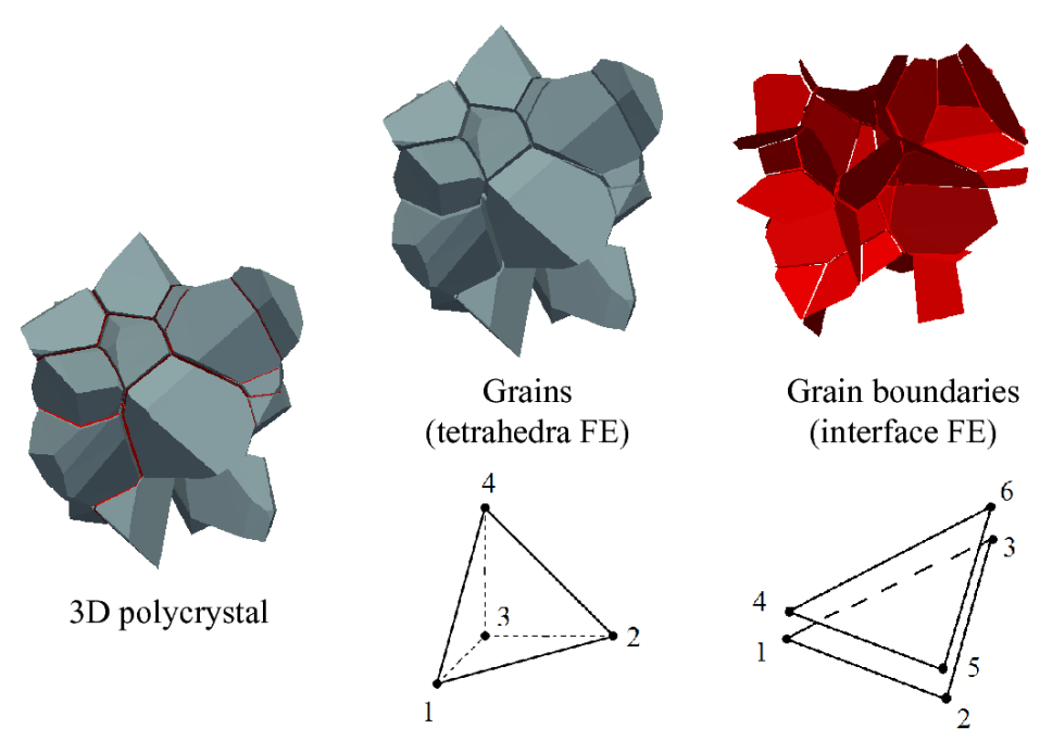
Figure 1: Matching of nodes along grain boundaries requires node duplication and a suitable data structure.

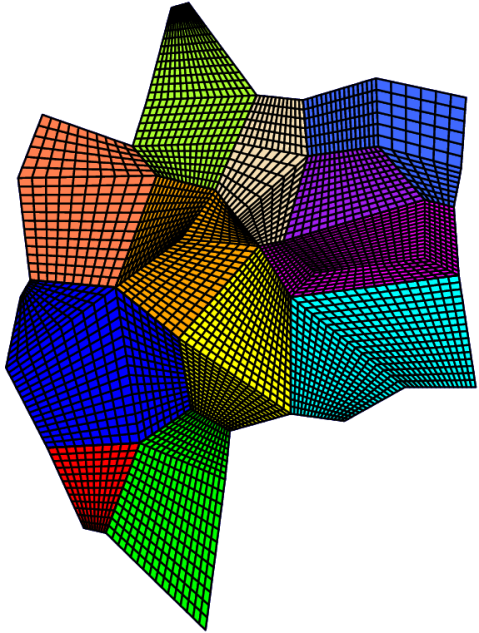
Figure 2: The constraint of matching nodes at grain boundaries can lead to non-uniform finite element meshes.

In composites, on the other hand, it is frequent to have material components with very different elastic properties. This is for instance the case of Aluminum metal-matrix composites reinforced by stiff ceramic fibers (Fig.3), or in the case of deformable polymeric layers bonded to a very stiff substrate, as for epoxy layers bonded on glass used in photovoltaic applications (Fig.4). The stiffer component of the composite system behaves almost as a rigid body with negligible deformation. Therefore, it would be computationally efficient to adopt a coarse finite element discretization for the rigid component, albeit keeping fine the finite element discretization of the interface and of the deformable material.

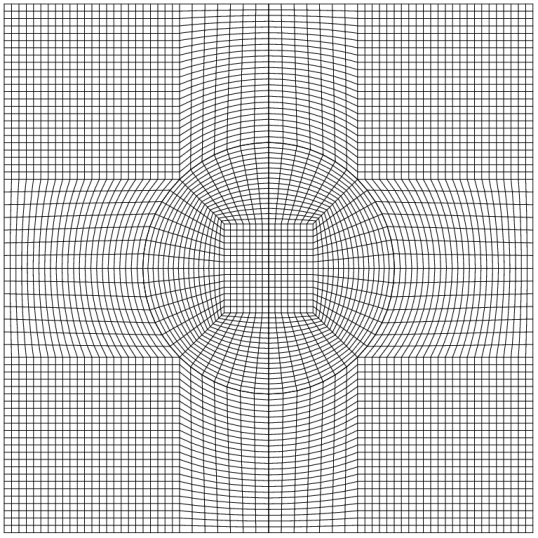
Figure 3: Fiber-reinforced metal-matrix composites: the fiber behaves almost as a rigid body and it could be discretized with a coarser finite element mesh than that used for the matrix.

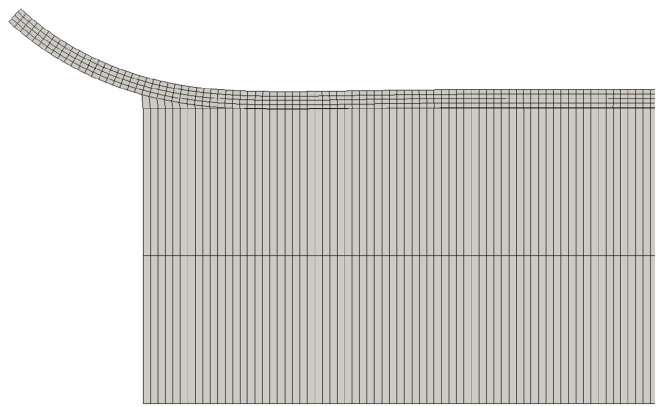
Figure 4: Peeling of a deformable layer from a stiff substrate: the substrate could be meshed with a coarser finite element mesh than that used for the layer.

In all of these problems, a much simpler and computationally more efficient mesh generation procedure would be to mesh each material region independently from the others and then insert interface elements along their internal boundaries capable to deal with non matching nodes. In the case of mesh adaptivity based on error control during nonlinear fracture mechanics simulations, the possibility of dealing with different mesh dicretizations of the continuum domains would also be very useful.

In the present study, we propose two new interface finite elements for interface fracture problems inspired by contact mechanics able to deal with non matching nodes: one for 2D applications and called node-to-segment interface element, and another for 3D simulations and called node-to-surface interface element. Their mathematical formulation and the matrix form for the finite element implementation are detailed in Sections 2 and 3. Section 4 presents the mesh generation algorithms to be used in conjunction with the new interface elements. Patch tests are discussed in Section 5 to show that the new elements are able to transfer a uniform stress state in the case of uniform loading. Simple but relevant numerical applications showing the capabilities of the new finite element formulations are finally discussed in Section 6. Conclusions and perspectives complete the article.

2 Continuum mechanics framework

In the small deformation setting, let us consider a pair of deformable bodies in the reference undeformed configuration $\mathscr{B}^{1}$, $\mathscr{B}^{2}$ $\subset\mathbb{R}^{n_{dim}}$, where $n_{dim}$ is equal to 2 or 3 for 2D or 3D problems, respectively. In general, both bodies are subject to volume forces $\mathbf{F}_{v}^{i}$ $(i=1,2)$, and to boundary conditions under the form of tractions, $\mathbf{t}^{i}=\hat{\mathbf{t}}^{i}$ $(i=1,2)$ on $\partial\mathscr{B}_{\mathbf{t}}^{i}$, and displacements, $\mathbf{u}^{i}=\hat{\mathbf{u}}^{i}$ $(i=1,2)$ on $\partial\mathscr{B}_{\mathbf{u}}^{i}$. The bodies might have different linear or nonlinear constitutive relations and material properties (see Fig.5).

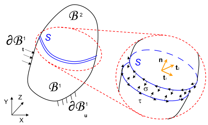
Figure 5: A sketch of two continuum bodies separated by a cohesive interface.

The interface between the deformable bodies is a region of lower spatial dimension denoted by $S\subset\mathbb{R}^{n_{dim}-1}$ where we allow displacement discontinuities, see Fig.5. Along the interface, defined by two opposing segments in 2D or facets in 3D, a local reference system can be introduced in relation to the modes of deformation of fracture mechanics, i.e., opening (or Mode I), sliding (or Mode II), and tearing (or Mode III).

Therefore, a normal vector $\mathbf{n}$ and a tangent vector $\mathbf{t}$ can be introduced along a 2D interface segment. Similarly, a normal vector $\mathbf{n}$ and two tangent vectors $\mathbf{t}_{1}$ and $\mathbf{t}_{2}$ can be defined along a 3D interface surface (see Fig.5). Since we are in the hypothesis of a zero-thickness interface and we are restricting our study to the small deformation setting, these vectors can be computed from the coordinates $\mathbf{x}$ of the nodes belonging to any of the two opposing segments or facets. Cohesive tractions opposing to the relative displacements can be interpreted in the framework of configurational forces [23], since their intensity and direction depend on the relative motion of the two bodies sharing the interface.

The virtual work of the interface tractions contribute to the Principle of Virtual Work of the whole system. This is the starting point to derive the finite element formulation. We recall that, for a standard interface element, we have:

$$\delta\Pi_{\mathrm{intf}}(\mathbf{u},\delta\mathbf{u})=\delta\mathbf{u}^{\mathrm{T}}\left[\int_{S_{0}}\left(\dfrac{\partial\mathbf{g}_{\mathrm{loc}}}{\partial\mathbf{u}}\right)^{\mathrm{T}}\,\mathbf{T}\mathrm{d}S\right],\hskip 5.69046pt\forall\delta\mathbf{u}\in\mathscr{V}\text{,}$$ (1)

where $\mathbf{g}_{\mathrm{loc}}$ is the gap vector that accounts for opening, sliding, and tearing displacements between the two sides of the interface and it represents the work conjugated magnitude to the cohesive tractions $\mathbf{T}$. The variable $\delta\mathbf{u}\in\mathscr{V}$ denotes the vector of the kinematically admissible virtual displacements.

3 Node-to-segment interface finite element

After introducing the finite element discretization of the two bodies sharing an interface by using linear triangular or quadrilateral elements, standard interface elements are assembled by pairing two opposing segments belonging to body 1 and 2, defined in terms of four nodes (see Fig.6(a)). Clearly, the use of these interface elements requires matching of the nodes of body 1 and body 2 at the common interface. At present, there is no method available in the literature to deal with non-conforming cohesive interfaces.

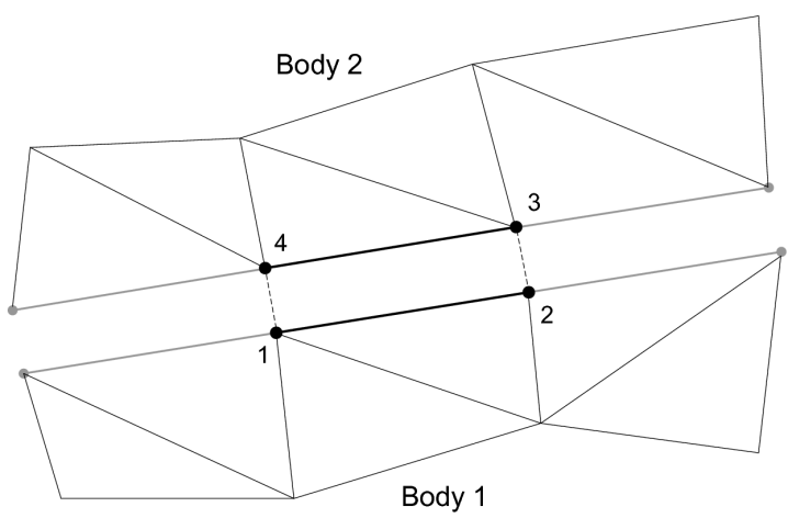
(a) Traditional interface element

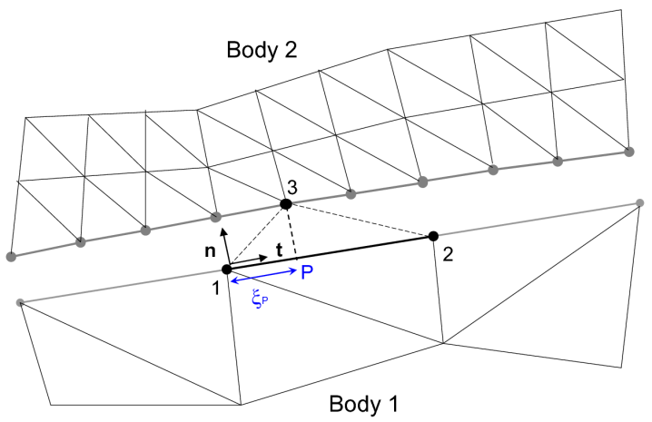
(b) Node-to-segment interface element

Figure 6: (a) Classical four-node interface element. (b) Proposed node-to-segment interface element.

To avoid this constraint, let’s define a new interface element relating the displacements of one node belonging to the boundary of the body 2 to the displacements of its projection normal to the corresponding segment belonging to the body 1, see Fig.6(b). We have therefore a topology analogous to a node-to-segment formulation used in contact mechanics [24], with the simplification that, in fracture mechanics applications under small displacements, pairing between the segment and the node has not to be updated during the simulation and it can be defined at the mesh generation stage.

For this interface element, the contribution to the Principle of Virtual Work reads:

$$\delta\Pi_{\mathrm{intf}}(\mathbf{u},\delta\mathbf{u})=\delta\mathbf{u}^{\mathrm{T}}\left(\dfrac{\partial\mathbf{g}_{\mathrm{loc},P}}{\partial\mathbf{u}}\right)^{\mathrm{T}}\,\mathbf{T}_{P}\,l_{el},\hskip 5.69046pt\forall\delta\mathbf{u}\in\mathscr{V}$$ (2)

where $\mathbf{g}_{\mathrm{loc},P}$ is the gap vector in the local reference system computed from the relative displacements of node 3 and of its projection $P$ on the segment $1-2$, and $\mathbf{T}_{P}$ is the corresponding traction vector function of the gaps according to the selected CZM. These quantities are multiplied by the length $l_{el}$, which is the area of influence of the node $3$ and is related to the finite element discretization of the interface from the side of body 2. The present formulation is valid for both structured and unstructured finite element meshes. More specifically, for each node belonging to the side of the interface having the finer discretization, which is the third node of each new interface element to be constructed according to the sketch in Fig.6(b), $l_{el}$ is computed as the sum of half the distances between that node and its closest neighbors. For edge nodes, only one neighbor has to be considered in the computation of $l_{el}$.

After introducing the finite element discretization, the continuum displacement vector $\mathbf{u}$ can be replaced by the nodal displacement vector $\mathbf{d}=(u_{1},v_{1},u_{2},v_{2},u_{3},v_{3})^{\mathrm{T}}$ in Eq.(2):

$$\delta\Pi_{\mathrm{intf}}(\mathbf{d},\delta\mathbf{d})=\delta\mathbf{d}^{\mathrm{T}}\left(\dfrac{\partial\mathbf{g}_{\mathrm{loc},P}}{\partial\mathbf{d}}\right)^{\mathrm{T}}\,\mathbf{T}_{P}\,l_{el}$$ (3)

This provides the expression of the element residual vector $\mathbf{f}^{e}$:

$$\mathbf{f}^{e}=\left(\dfrac{\partial\mathbf{g}_{\mathrm{loc},P}}{\partial\mathbf{d}}\right)^{\mathrm{T}}\,\mathbf{T}_{P}\,l_{el}$$ (4)

The local gap vector in the point $P$, $\mathbf{g}_{\mathrm{loc},P}=(g_{n},g_{t})_{P}^{\mathrm{T}}$, can be determined from the nodal displacement vector as follows:

$$\mathbf{g}_{\mathrm{loc},P}=\mathbf{R}\mathbf{B}_{P}\mathbf{d},$$ (5)

where $\mathbf{R}$ is the rotation matrix defined in terms of the unit vectors $\mathbf{n}=(n_{x},n_{y})^{\mathrm{T}}$ and $\mathbf{t}=(t_{x},t_{y})^{\mathrm{T}}$ that are related to the coordinates of the nodes 1 and 2, see Appendix for their explicit expressions:

$$\mathbf{R}=\left[\begin{array}[]{cc}n_{x}&n_{y}\\ t_{x}&t_{y}\\ \end{array}\right]$$ (6)

The operator $\mathbf{B}_{P}$ is defined as:

$$\mathbf{B}_{P}=\left[\begin{array}[]{cccccc}-N_{1}&0&-N_{2}&0&1&0\\ 0&-N_{1}&0&-N_{2}&0&1\\ \end{array}\right]_{P}$$ (7)

where $N_{1}=\xi/l$ and $N_{2}=(1-\xi/l)$ are the linear shape functions for the nodes $1$ and $2$, dependent on the surface coordinate $\xi$ as in Fig.6(b). The length $l$ is defined by $l=\|\mathbf{x}_{2}-\mathbf{x}_{1}\|$. The shape functions have to be computed in correspondence to the point $P$, i.e., for $\xi_{P}=(\mathbf{x}_{3}-\mathbf{x}_{1})\cdot\mathbf{t}$.

Introducing Eq.(5) into Eq.(3), the final matrix form for the element residual vector is derived:

$$\mathbf{f}^{e}=\mathbf{B}_{P}^{\mathrm{T}}\,\mathbf{R}^{\mathrm{T}}\mathbf{T}_{P}\,l_{el}$$ (8)

The element tangent stiffness matrix for an implicit solution scheme is computed by performing a consistent linearization of the residual:

$$\mathbf{K}^{e}=\dfrac{\partial\mathbf{f}^{e}}{\partial\mathbf{d}}=\mathbf{B}_{P}^{\mathrm{T}}\,\mathbf{R}^{\mathrm{T}}\dfrac{\partial\mathbf{T}_{P}}{\partial\mathbf{d}}\,l_{el}$$ (9)

where $\partial\mathbf{T}_{P}/\partial\mathbf{d}$ is obtained by a chain rule differentiation:

$$\dfrac{\partial\mathbf{T}_{P}}{\partial\mathbf{d}}=\dfrac{\partial\mathbf{T}_{P}}{\partial\mathbf{g}_{\mathrm{loc},P}}\dfrac{\partial\mathbf{g}_{\mathrm{loc},P}}{\partial\mathbf{d}}=\mathbf{C}_{P}\mathbf{R}\mathbf{B}_{P}$$ (10)

The tangent constitutive matrix $\mathbf{C}_{P}$ depends on the form of the cohesive traction-separation relation $\mathbf{T}=(\sigma,\tau)^{\mathrm{T}}$ vs. $\mathbf{g}_{\mathrm{loc}}=(g_{n},g_{t})^{\mathrm{T}}$, i.e., on the CZM expression. Its symbolic form reads:

$$\mathbf{C}_{P}=\left[\begin{array}[]{cccc}\dfrac{\partial\sigma}{\partial g_{n}}&\dfrac{\partial\sigma}{\partial g_{t}}\\ \dfrac{\partial\tau}{\partial g_{n}}&\dfrac{\partial\tau}{\partial g_{t}}\\ \end{array}\right]_{P}$$ (11)

It has to be remarked that the proposed node-to-segment interface element satisfies the internal rotational equilibrium, while the standard 4-nodes interface element does not, as pointed out in [25].

4 Node-to-surface interface finite element

For 3D problems, like for intergranular crack propagation in polycrystalline materials studied in [12], the finite element discretization of the bulk is usually performed by using tetrahedra finite elements, due to the high versatility in meshing complex polyhedral domains. In case of linear tetrahedra, standard interface elements are linking the edges of two tetrahedra and are represented by two triangles in 3D with 3 nodes each. A sketch of this standard interface element is shown in Fig.7(a).

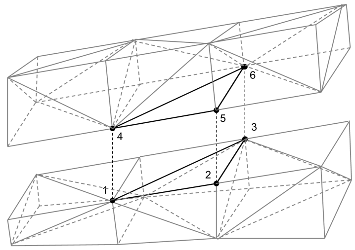
(a) Traditional interface element

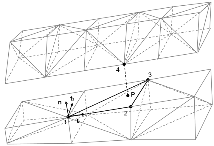
(b) Node-to-surface interface element

Figure 7: (a) classical six-node interface element. (b) Proposed node-to-surface interface element.

For different structured finite element discretizations of the two bodies, it is convenient to introduce a new interface element that relates the displacements of one node belonging to the boundary of body 2 to the displacements of its projection normal to the corresponding triangular facet belonging to body 1, see Fig.7(b). We have therefore a topology analogous to a node-to-surface formulation used in contact mechanics [24], again with fixed pairing defined during mesh generation due to the small displacement scenario.

For this interface element, the contribution to the Principle of Virtual Work reads:

$$\delta\Pi_{\mathrm{intf}}(\mathbf{u},\delta\mathbf{u})=\delta\mathbf{u}^{\mathrm{T}}\left(\dfrac{\partial\mathbf{g}_{\mathrm{loc},P}}{\partial\mathbf{u}}\right)^{\mathrm{T}}\,\mathbf{T}_{P}\,A_{el}k,\quad\forall\delta\mathbf{u}\in\mathscr{V}$$ (12)

where $\mathbf{g}_{\mathrm{loc},P}$ is related to the relative displacements of node 4 and of its projection $P$ onto the facet $1-2-3$. $\mathbf{T}_{P}$ is the corresponding traction vector given by the CZM relation. For each interface element, these quantities are multiplied by the area $A_{el}$ and by the coefficient $k$. For structured interface discretizations, $A_{el}$ is the area of any of the $e$ facets converging to the node 4 on the side of the interface having the finer discretization. The coefficient $k$ can be computed as the ratio between the number $e$ of facets converging to the node 4, divided by three times the number $q$ of facets belonging to the opposite side of the interface (having the coarser discretization) with minimum distance from the node 4. The number $q$ is typically equal to 1 if the normal projection of node 4 to the opposite side of the interface is inside a facet, or is equal to 2 if it falls on the edge between two adjoining facets. Edge nodes are treated in the same way as the internal nodes. A practical example showing the various possible cases is illustrated in the next section which treats the algorithms for mesh generation in the 2D and in the 3D cases.

After introducing the finite element discretization, we can replace the continuum displacement vector $\mathbf{u}$ with the nodal displacement vector $\mathbf{d}=(u_{1},v_{1},w_{1},u_{2},v_{2},w_{2},u_{3},v_{3},w_{3})^{\mathrm{T}}$ in Eq.(12):

$$\delta\Pi_{\mathrm{intf}}(\mathbf{d},\delta\mathbf{d})=\delta\mathbf{d}^{\mathrm{T}}\left(\dfrac{\partial\mathbf{g}_{\mathrm{loc},P}}{\partial\mathbf{d}}\right)^{\mathrm{T}}\,\mathbf{T}_{P}\,A_{el}k$$ (13)

which provides the expression of the element residual vector $\mathbf{f}^{e}$:

$$\mathbf{f}^{e}=\left(\dfrac{\partial\mathbf{g}_{\mathrm{loc},P}}{\partial\mathbf{d}}\right)^{\mathrm{T}}\,\mathbf{T}_{P}\,A_{el}k$$ (14)

The local gap vector in the point $P$, $\mathbf{g}_{\mathrm{loc},P}=(g_{n},g_{t1},g_{t2})_{P}^{\mathrm{T}}$, can be determined from the nodal displacement vector, see Eq.(5), where $\mathbf{R}$ is now a rotation matrix defined in terms of the unit vectors $\mathbf{n}=(n_{x},n_{y},n_{z})^{\mathrm{T}}$, $\mathbf{t}_{1}=(t_{1x},t_{1y},t_{1z})^{\mathrm{T}}$, and $\mathbf{t}_{2}=(t_{2x},t_{2y},t_{2z})^{\mathrm{T}}$, see Fig.7(b):

$$\mathbf{R}=\left[\begin{array}[]{ccc}n_{x}&n_{y}&n_{z}\\ t_{1x}&t_{1y}&t_{1z}\\ t_{2x}&t_{2y}&t_{2z}\\ \end{array}\right]$$ (15)

The components of $\mathbf{R}$ can be related to the coordinates of the nodes 1, 2, and 3, $\mathbf{x}_{i}=(x_{i},y_{i},z_{i})^{\mathrm{T}}$ $(i=1,2,3)$, see the expressions in the Appendix.

The operator $\mathbf{B}_{P}$ is defined as:

$$\mathbf{B}_{P}=\left[\begin{array}[]{cccccccccccc}-N_{1}&0&0&-N_{2}&0&0&-N_{3}&0&0&1&0&0\\ 0&-N_{1}&0&0&-N_{2}&0&0&-N_{3}&0&0&1&0\\ 0&0&-N_{1}&0&0&-N_{2}&0&0&-N_{3}&0&0&1\\ \end{array}\right]_{P}$$ (16)

where linear shape functions $N_{1}$, $N_{2}$, and $N_{3}$ are introduced to interpolate the nodal quantities over the $1-2-3$ plane. Denoting with $\mathbf{x}^{*}=(\xi,\eta,s)^{\mathrm{T}}$ the coordinates in the local reference system defined by the local frame $\mathbf{n}$, $\mathbf{t}_{1}$ and $\mathbf{t}_{2}$ with origin in the node $1$, obtained by pre-multiplying the vectors $(\mathbf{x}-\mathbf{x}_{1})$ by the rotation matrix $\mathbf{R}$, $\mathbf{x}^{*}=\mathbf{R}(\mathbf{x}-\mathbf{x}_{1})$, we can write

$$N_{1} =a_{1}\xi+b_{1}\eta+c_{1}$$ (17a)

$$N_{2} =a_{2}\xi+b_{2}\eta+c_{2}$$ (17b)

$$N_{3} =a_{3}\xi+b_{3}\eta+c_{3}$$ (17c)

with coefficients $a_{i}$, $b_{i}$, and $c_{i}$ $(i=1,2,3)$:

$$a_{1} =\dfrac{\eta_{2}-\eta_{3}}{\xi_{2}\eta_{3}-\eta_{2}\xi_{3}},\quad b_{1}=\dfrac{\xi_{3}-\xi_{2}}{\xi_{2}\eta_{3}-\eta_{2}\xi_{3}},\quad c_{1}=1$$

$$a_{2} =\dfrac{\eta_{3}}{\xi_{2}\eta_{3}-\eta_{2}\xi_{3}},\quad b_{2}=-\dfrac{\xi_{3}}{\xi_{2}\eta_{3}-\eta_{2}\xi_{3}},\quad c_{2}=0$$

$$a_{3} =-\dfrac{\eta_{2}}{\xi_{2}\eta_{3}-\eta_{2}\xi_{3}},\quad b_{3}=\dfrac{\xi_{2}}{\xi_{2}\eta_{3}-\eta_{2}\xi_{3}},\quad c_{3}=0$$

Note that the shape functions entering the matrix $\mathbf{B}_{P}$ in Eq.(16) have to be computed with respect to the coordinates of the point $P$, i.e., for $\xi=\xi_{4}$ and $\eta=\eta_{4}$.

Introducing the expression for the gap into Eq.(13) we obtain:

$$\mathbf{f}^{e}=\mathbf{B}_{P}^{\mathrm{T}}\,\mathbf{R}^{\mathrm{T}}\mathbf{T}_{P}\,A_{el}k$$ (19)

The element tangent stiffness matrix is derived from the consistent linearization of the element residual vector:

$$\mathbf{K}^{e}=\dfrac{\partial\mathbf{f}^{e}}{\partial\mathbf{d}}=\mathbf{B}_{P}^{\mathrm{T}}\,\mathbf{R}^{\mathrm{T}}\dfrac{\partial\mathbf{T}_{P}}{\partial\mathbf{d}}\,A_{el}k$$ (20)

where $\partial\mathbf{T}_{P}/\partial\mathbf{d}$ is computed by a chain rule differentiation:

$$\dfrac{\partial\mathbf{T}_{P}}{\partial\mathbf{d}}=\dfrac{\partial\mathbf{T}_{P}}{\partial\mathbf{g}_{\mathrm{loc},P}}\dfrac{\partial\mathbf{g}_{\mathrm{loc},P}}{\partial\mathbf{d}}=\mathbf{C}_{P}\mathbf{R}\mathbf{B}_{P}$$ (21)

The tangent constitutive matrix $\mathbf{C}_{P}$ depends on the form of the cohesive traction-separation relation $\mathbf{T}=(\sigma,\tau_{1},\tau_{2})^{\mathrm{T}}$ vs. $\mathbf{g}_{\mathrm{loc}}=(g_{n},g_{t1},g_{t2})^{\mathrm{T}}$, i.e., on the CZM expression. Its symbolic form reads:

$$\mathbf{C}_{P}=\left[\begin{array}[]{cccc}\dfrac{\partial\sigma}{\partial g_{n}}&\dfrac{\partial\sigma}{\partial g_{t1}}&\dfrac{\partial\sigma}{\partial g_{t2}}\\ \dfrac{\partial\tau_{1}}{\partial g_{n}}&\dfrac{\partial\tau_{1}}{\partial g_{t1}}&\dfrac{\partial\tau_{1}}{\partial g_{t2}}\\ \dfrac{\partial\tau_{2}}{\partial g_{n}}&\dfrac{\partial\tau_{2}}{\partial g_{t1}}&\dfrac{\partial\tau_{2}}{\partial g_{t2}}\end{array}\right]_{P}$$ (22)

As for the node-to-segment interface element is concerned, also this node-to-surface interface element satisfies the internal rotational and torsional equilibrium in addition to the translational one, while standard interface elements do not.

5 Mesh generation procedures for the new interface elements

Since the proposed interface elements do not require the same finite element discretization on both sides of the interface, the operations of mesh generation can be highly simplified with respect to standard interface elements. Material domains can be meshed independently from each other, with different finite element discretizations. In the case of structured meshes with uniform mesh size on both sides of the interface, then we can call $h_{1}$ and $h_{2}$ the interface mesh sizes of body 1 and body 2, respectively. This is a common situation resulting from mesh generators when the number of divisions/element size are specified by the user for the internal boundaries. After meshing the domains, nodes belonging to different material regions should not be tied. We also remark that the present node-to-segment interface element formulation can also comply with non-structured finite element meshes.

In the case of node-to-segment interface elements, see Fig.8, mesh generation can be implemented via a loop over the nodes $i$ belonging to the set $\mathcal{I}_{n}$ of the elements discretizing the boundary of body 2. The numerosity of this set is $\#\mathcal{I}_{n}=n$ and the distance between two consecutive nodes is $l$. On the opposite side of the interface it is possible to identify a set of segments $\mathcal{I}_{m}$ belonging to body 1, with numerosity $\#\mathcal{I}_{m}=m$. In the sketch in Fig.8 we have for instance $n=7$ and $m=2$ and the ratio between element sizes is $h_{1}/h_{2}=3$. For each node $i\in\mathcal{I}_{n}$, the problem is to find the segment $m\in\mathcal{I}_{m}$ having the minimum distance from $i$. The connectivity matrix of the node-to-segment finite element to be generated will be composed by the node numbers defining the segment, plus the number of the node $i$. If a node has two segments with the same minimal distance, then two interface elements have to be assembled, one for each segment. For instance, in the example in Fig.8, the node 4 has to be paired with the segment $m=1$ (defined by the nodes 8 and 9) and with the segment $m=2$ (defined by the nodes 9 and 10).

In the case of structured meshes, the length of influence of the nodes, $l_{el}$, is equal to $l/3$ for $i=2,\dots,6$, and it is equal to $l/6$ for the boundary nodes $i=1$ and $i=7$, see Fig.8. For unstructured meshes, on the other hand, $l_{el}$ varies from node to node and it is equal to the sum of half the distances between that node and its two neighbors. For edge nodes, only one half a distance with its neighbor has to be computed. The operations of the 2D mesh generation procedure are summarized in Algorithm 1.

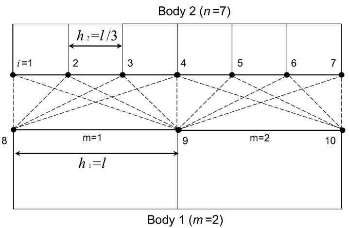
Figure 8: An example showing 2D interface mesh generation with node-to-segment interface elements.

    Input: set of nodes $\mathcal{I}_{n}$ belonging to the interface of body 2 $(\#\mathcal{I}_{n}=n)$; set of segments $\mathcal{I}_{m}$ $(\#\mathcal{I}_{m}=m)$ of the interface discretization of body 1.  

1. LOOP $i=1,\dots,n$

   1. Compute the length of influence of the node $i$, $l_{el}$, as the sum of half the distances between the node $i$ and its neighboring nodes. For an edge node, only one neighbor exists;

   2. Determine the number $q$ of segments of the set $\mathcal{I}_{m}$ with minimum distance from the node $i$;

   3. LOOP $j=1,\dots,q$

   4. Determine the node numbers defining the segment $j$;

   5. Construct the connectivity matrix of the interface element as a list of nodes defining the segment $j$, plus the node $i$;

   6. END LOOP

2. END LOOP

    Output: Connectivity matrix of the node-to-segment interface elements to pair different structured or unstructured finite element meshes of the continuum.  

Algorithm 1 2D interface mesh generation algorithm

Mesh generation in 3D requires again a loop over the nodes $i\in\mathcal{I}_{n}$. We consider here for the sake of simplicity structured mesh discretizations of the bulk realized with linear tetrahedra having a uniform mesh size from each side of the interface, $h_{1}$ and $h_{2}$, for body 1 and body 2, respectively. The area $A_{el}$ is related to $h_{2}$ and its corresponds to the area of any facet converning to $i$, see the example in Fig.9.

For each node $i$, the facet $m$ of the finite element belonging to the interface of body 1, with minimal distance from $i$, is determined. In the most general case, there is a single facet $m$ corresponding to the node $i$ $(q=1)$ and the mesh parameter $k$ has simply to be set equal to the number of finite elements $e$ on the interface surface of body 2 converging into the node $i$, divided by 3. This is for instance the case of all the nodes displayed in blue in Fig.9. On the other hand, if the orthogonal projection of the node $i$ onto the interface of body 1 belongs to a boundary between two facets, then $q=2$ and two node-to-surface interface elements have to be paired and assembled, one for each facet. In this case the parameter $k$ is equal to the number of finite elements on the interface surface of body 2 converging to the node $i$, divided by $q$ and by 3. This is for instance the case of the nodes displayed in black in Fig.9 (please refer to the online version for colors). These operations are summarized in Algorithm 2.

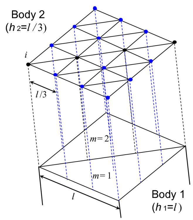
Figure 9: An example showing 3D interface mesh generation with node-to-surface interface elements: black nodes have their orthogonal projection to the interface onto an internal edge. They will require assembling of two interface elements, one for the facet $m=1$, and another for the facet $m=2$.

    Input: set of nodes $\mathcal{I}_{n}$ belonging to the interface of body 2 $(\#\mathcal{I}_{n}=n)$; set of facets $\mathcal{I}_{m}$ $(\#\mathcal{I}_{m}=m)$ of the interface discretization of body 1.  

1. LOOP $i=1\dots,n$

   1. Compute the area of a generic facet, $A_{el}$;

   2. Determine the number $e$ of facets belonging to the interface of body 2 and converging to the node $i$;

   3. Determine the number $q$ of facets of the set $\mathcal{I}_{m}$ with minimum distance from the node $i$;

   4. $k\leftarrow e/(3q)$

   5. LOOP $j=1,\dots,q$

   6. Determine the node numbers defining the facet;

   7. Construct the connectivity matrix of the interface element as a list of the nodes of the facet $j$, plus the node $i$;

   8. END LOOP

2. END LOOP

    Output: Connectivity matrix of the node-to-surface interface elements.  

Algorithm 2 3D interface mesh generation algorithm

6 Patch tests

The patch test is performed to show the capability of the proposed elements to transfer a uniform stress field across an interface in the case of a uniform loading. Let us consider two blocks of horizontal side $a=1$ m, and vertical side $b=0.5$ m, made of the same material and separated by a cohesive interface. Young’s modulus of the bulk is $E=10$ GPa and its Poisson ratio is $\nu=0$. The lower block is constrained to vertical displacements along its lower side. One node along the same side is also constrained to horizontal displacements to avoid rigid body motion. A vertical displacement $\Delta$ is imposed to the upper side of the second block, in order to induce Mode I decohesion at the interface whose traction-separation relation is ruled by the Tvergaard CZM [5]. In that CZM, tractions are explicit nonlinear functions of the relative opening and sliding displacements $g_{n}$ and $g_{t}$:

$$\sigma= \sigma_{\max}\dfrac{g_{n}}{g_{\text{nc}}}P(\lambda)$$ (23a)

$$\tau= \tau_{\max}\dfrac{g_{t}}{g_{\text{tc}}}P(\lambda)$$ (23b)

where $g_{nc}$ and $g_{tc}$ are the critical opening and sliding displacements corresponding to complete decohesion under pure Mode I or Mode II deformation, respectively. The function $P(\lambda)$ reads:

$$P(\lambda)= \left\{\begin{array}[]{ll}\dfrac{27}{4}\left(1-2\lambda+\lambda^{2}\right),&\text{for}\,0\leq\lambda\leq 1\\ 0,&\text{otherwise}\end{array}\right.$$ (24c)

$$\lambda= \sqrt{\left(\dfrac{g_{n}}{g_{nc}}\right)^{2}+\left(\dfrac{g_{t}}{g_{tc}}\right)^{2}}$$ (24d)

For this CZM, the tangent constitutive matrix $\mathbf{C}_{P}$ has the following expression:

$$\mathbf{C}_{P}= \left[\begin{array}[]{cc}\sigma_{\max}\dfrac{P}{g_{nc}}+\sigma_{\max}\dfrac{g_{n}}{g_{nc}}\dfrac{\partial P}{\partial\lambda}\dfrac{\partial\lambda}{\partial g_{n}}&\sigma_{\max}\dfrac{g_{n}}{g_{nc}}\dfrac{\partial P}{\partial\lambda}\dfrac{\partial\lambda}{\partial g_{t}}\\ \tau_{\max}\dfrac{g_{t}}{g_{tc}}\dfrac{\partial P}{\partial\lambda}\dfrac{\partial\lambda}{\partial g_{n}}&\tau_{\max}\dfrac{P}{g_{tc}}+\tau_{\max}\dfrac{g_{t}}{g_{tc}}\dfrac{\partial P}{\partial\lambda}\dfrac{\partial\lambda}{\partial g_{t}}\end{array}\right]_{P}$$ (25)

In 3D, the effective displacement $\lambda$ is computed as follows:

$$\lambda=\sqrt{\left(\dfrac{g_{n}}{g_{nc}}\right)^{2}+\left(\dfrac{g_{t1}}{g_{tc}}\right)^{2}+\left(\dfrac{g_{t2}}{g_{tc}}\right)^{2}}$$ (26)

and the cohesive tractions are:

$$\sigma= \sigma_{\max}\dfrac{g_{n}}{g_{nc}}P(\lambda),$$ (27a)

$$\tau_{1}= \tau_{\max}\dfrac{g_{t1}}{g_{tc}}P(\lambda),$$ (27b)

$$\tau_{2}= \tau_{\max}\dfrac{g_{t2}}{g_{tc}}P(\lambda).$$ (27c)

Similarly, the constitutive matrix $\mathbf{C}_{P}$ reads:

$$\mathbf{C}_{P}= \left[\begin{array}[]{ccc}\sigma_{\max}\dfrac{P(\lambda)}{g_{nc}}+\sigma_{\max}\dfrac{g_{n}}{g_{nc}}\dfrac{\partial P(\lambda)}{\partial\lambda}\dfrac{\partial\lambda}{\partial g_{n}}&\sigma_{\max}\dfrac{g_{n}}{g_{nc}}\dfrac{\partial P(\lambda)}{\partial\lambda}\dfrac{\partial\lambda}{\partial g_{t1}}&\sigma_{\max}\dfrac{g_{n}}{g_{nc}}\dfrac{\partial P(\lambda)}{\partial\lambda}\dfrac{\partial\lambda}{\partial g_{t2}}\\ \tau_{\max}\dfrac{g_{t1}}{g_{tc}}\dfrac{\partial P(\lambda)}{\partial\lambda}\dfrac{\partial\lambda}{\partial g_{n}}&\tau_{\max}\dfrac{P(\lambda)}{g_{tc}}+\tau_{\max}\dfrac{g_{t1}}{g_{tc}}\dfrac{\partial P(\lambda)}{\partial\lambda}\dfrac{\partial\lambda}{\partial g_{t1}}&\tau_{\max}\dfrac{g_{t1}}{g_{tc}}\dfrac{\partial P(\lambda)}{\partial\lambda}\dfrac{\partial\lambda}{\partial g_{t2}}\\ \tau_{\max}\dfrac{g_{t2}}{g_{tc}}\dfrac{\partial P(\lambda)}{\partial\lambda}\dfrac{\partial\lambda}{\partial g_{n}}&\tau_{\max}\dfrac{g_{t2}}{g_{tc}}\dfrac{\partial P(\lambda)}{\partial\lambda}\dfrac{\partial\lambda}{\partial g_{t1}}&\tau_{\max}\dfrac{P(\lambda)}{g_{tc}}+\tau_{\max}\dfrac{g_{t2}}{g_{tc}}\dfrac{\partial P(\lambda)}{\partial\lambda}\dfrac{\partial\lambda}{\partial g_{t2}}\end{array}\right]_{P}$$ (28)

For the tests we select $\sigma_{\max}=10$ Pa, $g_{nc}=g_{tc}=0.3$ m, $\tau_{\max}/\sigma_{\max}=0$. Using these mechanical parameters, the interface is more compliant than the bulk and we obtain $g_{n}\sim\Delta$ at each time step. The corresponding stress field has to be uniform for equilibrium considerations.

The contour plots in Fig.10 obtained with $\Delta=0.2$ m show the vertical displacement field $v$ on the left and the vertical stress field $\sigma_{y}$ on the right, for different mesh discretizations. Figs.10(a) and 10(b) refer to the classical 4-nodes interface element where matching of nodes at the interface is required. Figs.10(c) and 10(d) correspond to different finite element discretizations of the two blocks done by linear quadrilateral elements, with $h_{1}/h_{2}=4$. To avoid the problem of having unmatched nodes at the interface, node-to-segment interface elements are used. The uniform stress field is correctly reproduced as in the case of a standard 4-nodes interface element, passing the patch test. The same problem is analyzed in Figs.10(e) and 10(f) with linear triangular elements used to discretize the continuum. Also in this case, with the same interface mesh generation procedure as before, the patch test is passed. Finally, we consider the case of non-structured finite element meshes, with a nonuniform finite element discretization, see Figs.10(g) and 10(h). In this case the length of influence of each node $l_{el}$ is different from node to node along the interface, as commented in the previous section.

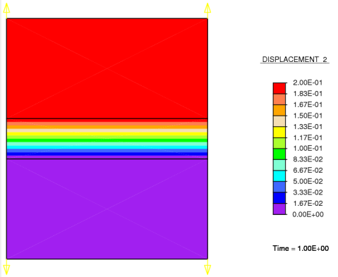
(a) $v$ (4-nodes interface el.)

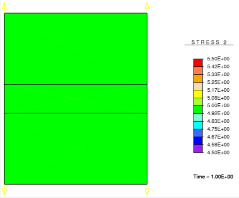
(b) $\sigma_{y}$ (4-nodes interface el.)

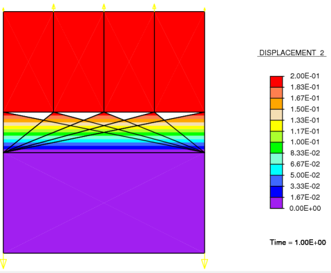
(c) $v$ ($h_{1}/h_{2}=4$)

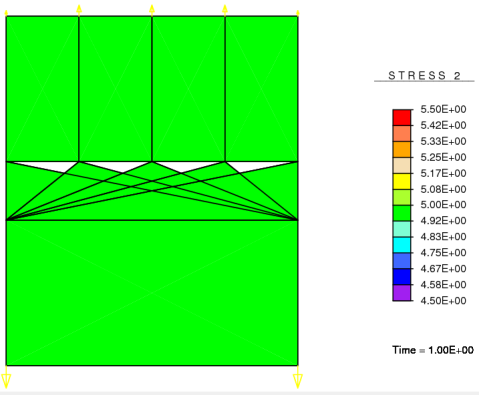
(d) $\sigma_{y}$ ($h_{1}/h_{2}=4$)

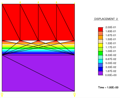
(e) $v$ ($h_{1}/h_{2}=4$)

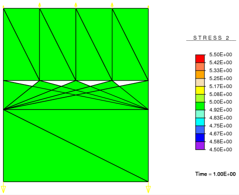
(f) $\sigma_{y}$ ($h_{1}/h_{2}=4$)

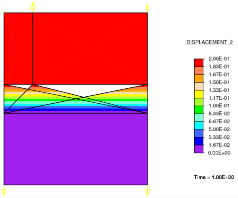
(g) $v$ (unstructured mesh)

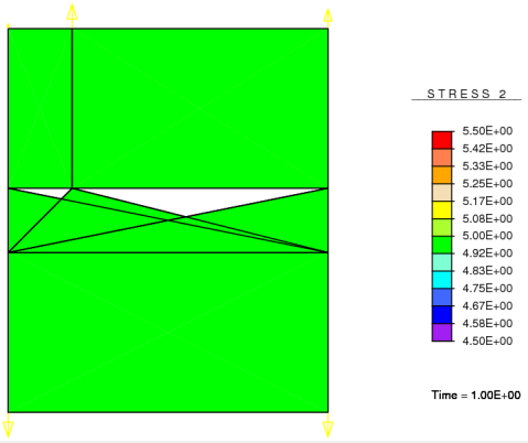
(h) $\sigma_{y}$ (unstructured mesh)

Figure 10: Patch test for the 2D node-to-segment interface element: the uniform stress field is obtained in tension. The benchmark solution corresponding to a standard 4-nodes interface element is shown in Figs.10(a) and 10(b). Figs.10(c) and 10(d) refer to a discretization with quadrilateral elements for the continuum; Figs. 10(e) and 10(f) refer to triangular elements; Figs. 10(g) and 10(h) correspond to unstructured finite element meshes.

The rate of convergence of the Newton-Raphson iterative scheme is shown in Fig.11 for the 4-nodes interface element (problem in Fig.10(a)) and for the node-to-segment interface element (problem in Fig.10(c)). In both cases quadratic convergence is achieved.

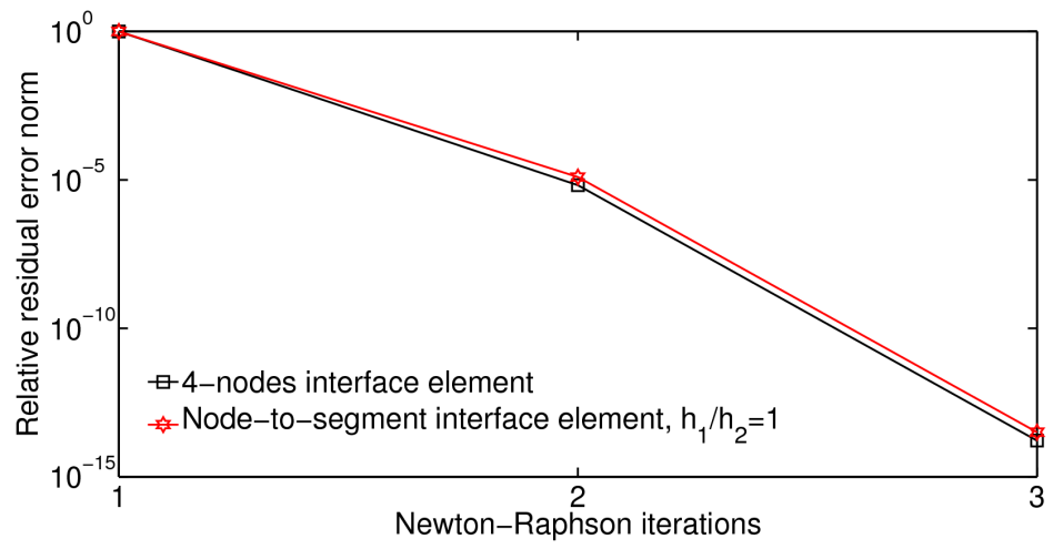
Figure 11: Convergence rate of the node-to-segment interface elements as compared to the standard 4-nodes interface element, for the mesh discretization of the bulk shown in Fig.10(a) and the same imposed boundary displacements.

The patch test is repeated for a 3D problem in Fig.12. A standard 8-nodes linear interface element is used in Fig.12(a) in case of matching nodes. The results for the same uniaxial test problem but with a different discretization of the blocks realized with linear tetrahedra $(h_{1}/h_{2}=3)$ are shown in Fig.12(b). The algorithm 2 was used to assemble the interface elements along the interface and the patch test is passed with a uniform stress field.

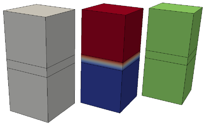
(a) Standard 8-nodes interface element

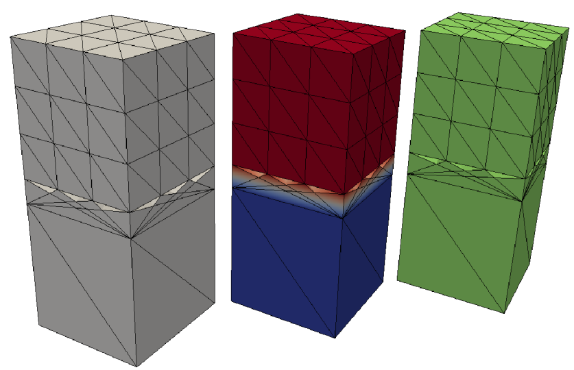
(b) Node-to-surface interface elements, $h_{1}/h_{2}=3$

Figure 12: Patch test of the 3D node-to-segment interface element: the uniform stress field is obtained in tension for different non-matching finite element discretizations of the interface. The pictures on the left show the finite element discretization, those in the middle show the displacement field in the $z$-direction, and those on the right show the vertical stress field in the $z$-direction.

7 Selected applications

In this section we present selected applications of the new interface elements to emphasize their usefulness and capabilities in relation to drawbacks of the standard interface elements pointed out in the introduction.

7.1 Peeling of deformable layers from rigid substrates

Let’s consider the problem of peeling of a deformable layer from a stiff substrate, see Fig.13. The numerical simulation of this problem requires a fine discretization of the deformable layer through its width to capture its bending deformation. The interface needs a fine discretization as well, to correctly resolve the cohesive tractions. On the other hand, a much coarser discretization for the substrate would be adequate, since it behaves almost as a rigid body. This is therefore a typical problem that could be efficiently handled by using two different mesh discretizations at the interface. An example of a finite element discretization by using standard 4-nodes interface elements, requiring matching of the nodes of the finite elements of body 1 and of body 2 at the interface, is shown in Fig.13(a). With the use of the node-to-segment interface elements we can keep fine the discretization of the deformable layer and we can coarsen the discretization of the substrate, see Fig.13(b) with $h_{1}/h_{2}=8$. The substrate is restrained along its base and a vertical displacement $\Delta$, linearly increasing with time, is imposed to the layer as shown in Fig.13. The peeling force $P$ is computed as a reaction force for each value of $\Delta$.

The Young’s modulus of the layer is $E_{2}=1\times 10^{5}$ Pa and that of the substrate is $E_{1}=1\times 10^{10}$ Pa. In spite of the simplicity of the test, the significant mismatch in the elastic properties and the nonuniform traction distribution along the interface during peeling provides a critical benchmark problem for testing the accuracy of the new element in predicting the global force-displacement curve and the local traction distribution along the interface.

The horizontal size of the blocks is $L=1$ m, and the widths of the substrate and of the layer are set equal to 0.4 m and 0.1 m, respectively. We consider the cohesive zone model by Tveergard [5] as detailed in the previous section, considering two cases: $(i)$ $\sigma_{\max}=30$ Pa, $g_{nc}=g_{tc}=0.1$ m, $\tau_{\max}/\sigma_{\max}=0$; $(ii)$ $\sigma_{\max}=30$ Pa, $g_{nc}=g_{tc}=0.1$ m, $\tau_{\max}/\sigma_{\max}=1$.

The peeling force vs. imposed displacement curves for the two cases and for the two different mesh discretizations in Fig.13 are shown in Fig.14. The solution based on the node-to-segment interface elements is the same as that for the classic 4-nodes interface element. However, note that the new formulation leads to a significant reduction of finite elements used to discretize the rigid block. In terms of computation time, in spite of the relative simplicity of this test problem, a gain of $18\%$ is achieved by using the discretization in Fig.13(b) with respect to that in Fig.13(a).

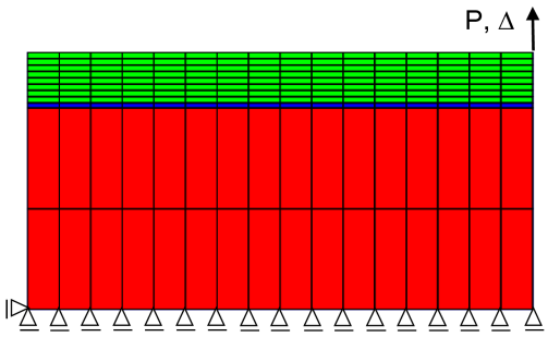
(a) Standard 4-nodes interface elements, $h_{1}/h_{2}=1$

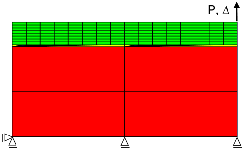
(b) Node-to-segment interface elements, $h_{1}/h_{2}=8$.

Figure 13: Finite element discretizations for the peeling test.

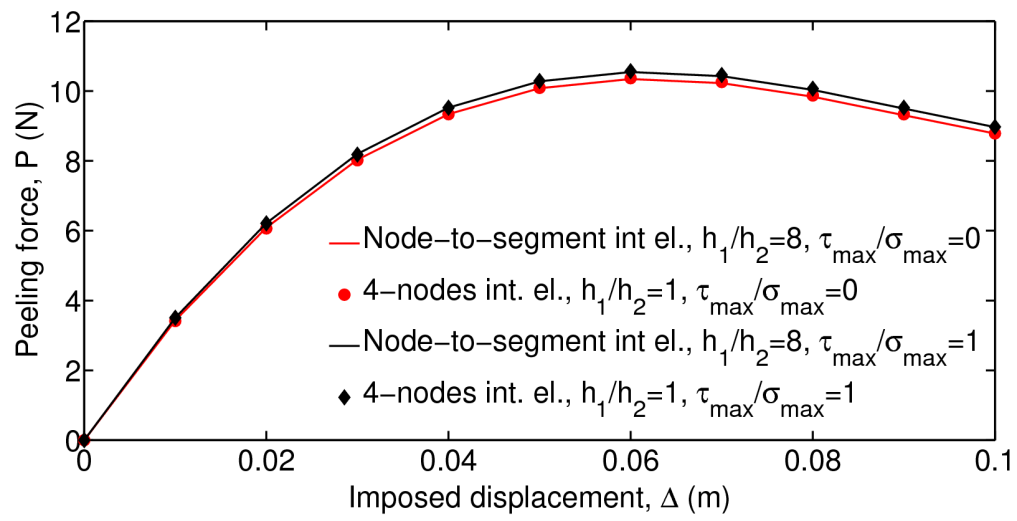
Figure 14: Force-displacement curves for the peeling test in Fig.13, for two different values of $\tau_{\max}/\sigma_{\max}$. Benchmark results obtained by using 4-nodes interface elements are shown with bullets.

The quality of the local solution can be assessed by examining the predicted effective dimensionless crack separation $\lambda$ and the normal and tangential cohesive tractions vs. $x/L$, where the variable $x$ defines the position along the interface ranging from $x/L=0$ at the left hand side up to $x/L=1$ at the right hand side. The results based on the node-to-segment interface element discretization are shown in Fig.15 for the previous test problem with $\tau_{\max}/\sigma_{\max}=1$, while the results based on the standard interface element discretization are shown with dots. The agreement between the two methods is excellent for all the interface quantities in the opening regime, i.e., for $g_{n}>0$. For the portion of the interface in contact near $x/L=0$, on the other hand, a difference in the distributions of the normal traction $\sigma$ is noticed. In the present framework, for both finite element discretization schemes, the contact constraint was enforced by the penalty method with a penalty parameter $\epsilon=1\times 10^{18}$ Pa/m. A possible improvement of the present work is expected by incorporating more accurate contact techniques like the mortar method [26, 27, 28, 29] in the interface element formulation, splitting the treatment of the contact stage from the debonding one.

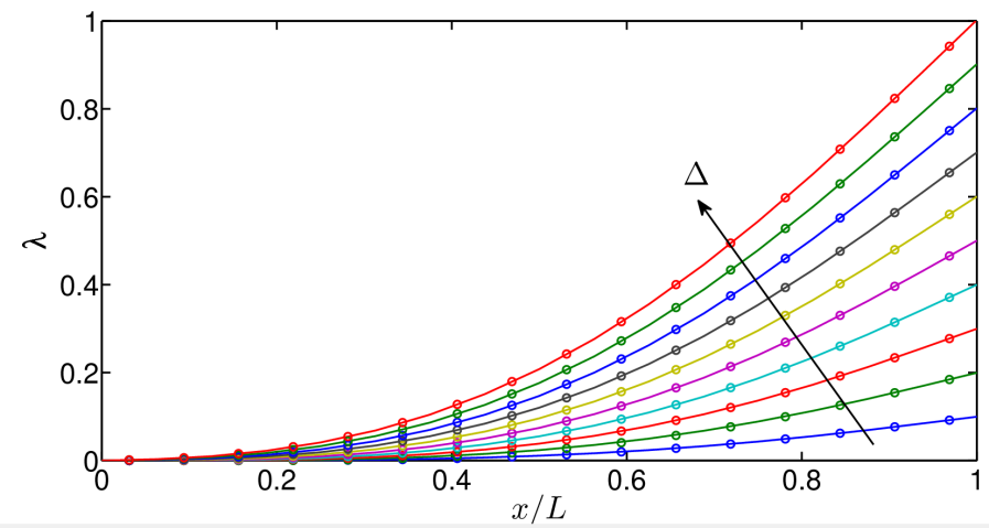
(a) Dimensionless separation, $\lambda$

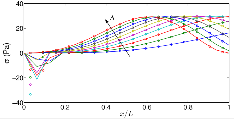
(b) Normal cohesive traction, $\sigma$

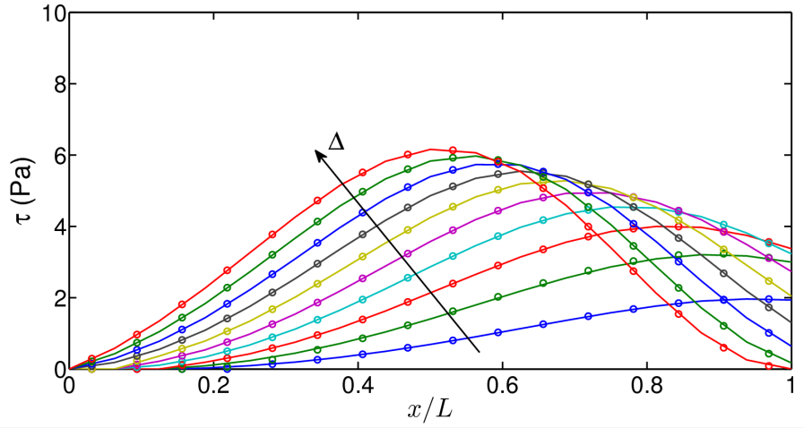
(c) Tangential cohesive traction, $\tau$

Figure 15: Local response of the proposed interface element (solid lines) vs. standard interface element (dots) for different far-field imposed displacements $\Delta$ in Fig. 14.

7.2 Modelling cohesive interfaces with non propagating crack tips

Another problem where the new interface elements can be useful concerns modelling cohesive interfaces whose tips are expected not to propagate. In reference to Fig.16, this can be the case of an interface between two strips shown in blue and green of 6 m height and 1 m width (please refer to the online version of this article for colors), fully bonded along vertical interfaces to two continuous external strips also 1 m width, shown in red. Assuming that the cohesive interface cannot propagate into the external layers and it cannot lead to debonding of the vertical interfaces, interface elements have to be inserted along the crack line only.

Apart from the possibility of using different mesh discretizations for the blue and the green strips dictated by error control procedures, treatment of the crack tips is also a problem to be deal with. In fact, if we use standard 4-nodes interface elements, the crack tip nodes have to be duplicated as well and, as a consequence, thin solid elements have to be inserted along a line inside the red layers till reaching the external boundaries, see the discretization in the bulk of the red layer on the left of the crack tip in Fig.16. The same takes place ahead of the opposite crack tip. The width of these elements cannot be set equal to zero, but has to be taken as small as possible to model a sharp crack tip. The elongated shape of the continuum elements ahead of the crack tip is of course not ideal as far as their accuracy is concerned.

This problem can be completely avoided without affecting the way the finite element discretization of the red strips is performed by using node-to-segment interface elements to deal with the crack tip dicretization. The regions corresponding to the different material domains can be meshed independently from each other and their common nodes tied everywhere, except between the blue and the green regions. Zero-thickness node-to-segment interface elements are then inserted along this interface by applying the Algorithm 1. Alternatively, classical interface elements can be used at this stage for the cohesive description of the crack. At the crack tip, on the other hand, the node-to-segment interface element able to work with three nodes, namely nodes 247 and 483 in Fig.16 (defining the segment) and the node 998 for the crack tip on the left, is used. Similarly, for the opposite crack tip, the nodes 493 and 494 (defining the segment) and the node 1000 for the crack tip are used to generate the other node-to-segment interface element. This avoids the duplication of the nodes 257 and 494 and hence the finite element discretization of the continuous red stripes is no longer affected by the presence of the crack.

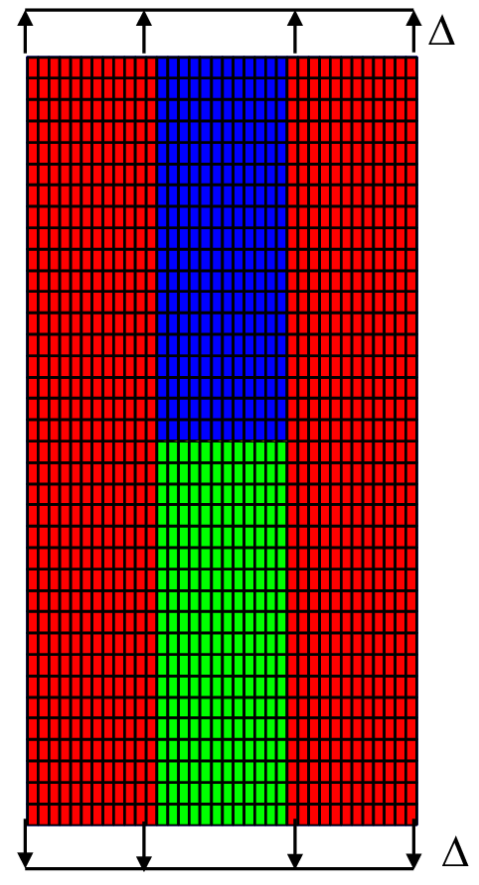
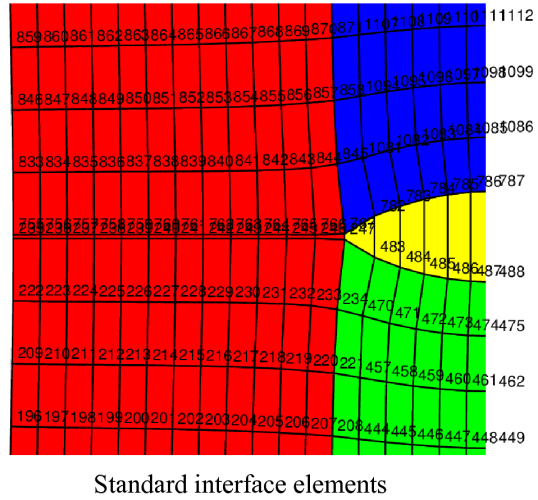
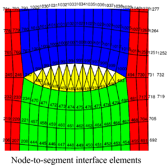
Figure 16: A central cohesive crack with non-propagating crack tips inserted into a composite elastic plate in tension.

The contour plots of the vertical displacement field are shown in Fig.17 for the sake of completeness, considering a Young’s modulus of the red strips equal to $2\times 10^{5}$ Pa, a Young’s modulus of the blue and green strips equal to $1\times 10^{5}$ Pa, vanishing Poisson’s ratios, CZM parameters $\sigma_{\max}=1000$ Pa, $\tau_{\max}/\sigma_{\max}=0$, $g_{n}=g_{t}=0.3$, and $\Delta=0.5$ m. The crack opening profile is exactly the same in the two cases.

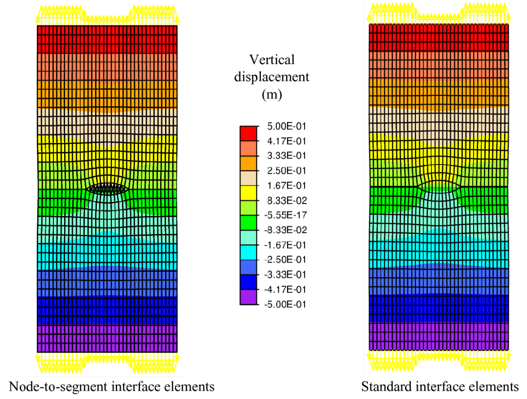
Figure 17: Contour plots of the vertical displacement field related to the problem in Fig.16, discretized with node-to-segment interface elements or with standard interface elements.

8 Conclusions and perspectives

Two novel interface elements have been proposed to discretize interfaces with non-matching nodes. The formulation is based on a particularization of node-to-segment and node-to-surface contact elements used in contact mechanics under the assumption of small displacements.

Mesh generation algorithms for 2D and 3D problems have also been presented, with a significant simplification over the classical meshing procedure required in the case of standard 2D and 3D interface elements. The proposed formulation allows the generation of finite element meshes of different bodies/material regions separately and depending on the needs, without the constraint of imposing the same finite element discretization at the interface. Therefore, the cumbersome procedure of meshing domains as fully bonded and then duplicating nodes at the interface can be completely avoided. This is particularly useful in the case of polygonal domains separated by cohesive interfaces, as in 2D and 3D polycrystalline materials, and in delamination problems where one material component is much stiffer than the other one, as in fiber-reinforced composites or in peeling tests of tapes from stiff substrates.

In terms of computational efficiency, uncoupling the mesh discretization of material regions allows a better control of mesh quality in computational materials science applications, and a selective reduction of number of finite elements in the case of fracture problems involving bodies with very different elastic properties. In the 2D peeling test, for instance, a saving of $18\%$ in computation time was achieved in spite of its coarse discretization. The local solution was also found quite accurate with respect to the standard interface element discretization, especially in terms of equivalent dimensionless gap and cohesive tractions along the portion of the interface experiencing debonding. In the part of the interface in contact, on the other hand, a discrepancy in the predictions has been observed. This suggests further developments of the proposed formulations by splitting the treatment of the debonding stage from the contact one. In the case of a negative crack opening (contact), the mortar method using dual spaces for the Lagrange multiplier [26] could be exploited. The mortar method introduces the continuity condition at interfaces in integral (global) form, rather than as nodal (local) constraints, with an improvement in the description of the contact predictions. This route is left for further developments and opens the possibility to create a new prototype of interface element able to deal with non-matching nodes during delamination and contact, particularly useful to accurately simulate cyclic loading conditions with alternating tension and compression stress states.

Finally, the second example has shown that the node-to-segment and the node-to-surface finite elements can used to discretize interface cracks with non-propagating crack tips. If employed to discretize the crack tips, then the finite element discretization of the neighboring material domains can be left completely unmodified, without the need of introducing continuum finite elements with very elongated shapes or changing the finite element discretization of the strips by using non uniform triangular meshes.

Acknowledgements

The research leading to these results has received funding from the European Research Council under the European Union’s Seventh Framework Programme (FP/2007-2013) / ERC Grant Agreement n. 306622 (ERC Starting Grant “Multi-field and multi-scale Computational Approach to Design and Durability of PhotoVoltaic Modules” - CA2PVM; PI: Prof. M. Paggi).

Appendix: coefficients entering the rotation matrices

For the node-to-segment interface element, the components of the normal and tangential unit vectors entering the definition of the rotation matrix $\mathbf{R}$ are related to the coordinates of the nodes 1 and 2, $\mathbf{x}_{i}=(x_{i},y_{i})^{\mathrm{T}}$ $(i=1,2)$, see Fig.6(b). Their expression is the following:

$$n_{x} =-\dfrac{y_{2}-y_{1}}{\|\mathbf{x}_{2}-\mathbf{x}_{1}\|}$$ (29a)

$$n_{y} =\dfrac{x_{2}-x_{1}}{\|\mathbf{x}_{2}-\mathbf{x}_{1}\|}$$ (29b)

$$t_{x} =\dfrac{x_{2}-x_{1}}{\|\mathbf{x}_{2}-\mathbf{x}_{1}\|}$$ (29c)

$$t_{y} =\dfrac{y_{2}-y_{1}}{\|\mathbf{x}_{2}-\mathbf{x}_{1}\|}$$ (29d)

For the node-to-surface interface element, on the other hand, the definition of the coefficients entering the rotation matrix requires to preliminary introduce the vectors $\mathbf{x}_{21}$ and $\mathbf{x}_{31}$ of components (see Fig. 7(b)):

$$x_{21} =x_{2}-x_{1},\quad y_{21}=y_{2}-y_{1},\quad z_{21}=z_{2}-z_{1}$$

$$x_{31} =x_{3}-x_{1},\quad y_{31}=y_{3}-y_{1},\quad z_{31}=z_{3}-z_{1}$$

After computing the area $A$ of the facet $1-2-3$:

$$A=\dfrac{\sqrt{(y_{21}z_{31}-z_{21}y_{31})^{2}+(z_{21}x_{31}-x_{21}z_{31})^{2}+(z_{21}y_{31}-y_{21}z_{31})^{2}}}{2}$$ (31)

the components of the normal and tangential unit vectors are finally provided by the following relations:

$$n_{x} =\dfrac{y_{21}z_{31}-z_{21}y_{31}}{2A}$$ (32a)

$$n_{y} =\dfrac{z_{21}x_{31}-x_{21}z_{31}}{2A}$$ (32b)

$$n_{z} =\dfrac{z_{21}y_{31}-y_{21}z_{31}}{2A}$$ (32c)

$$t_{1x} =\dfrac{x_{21}}{\sqrt{x_{21}^{2}+y_{21}^{2}+z_{21}^{2}}}$$ (32d)

$$t_{1y} =\dfrac{y_{21}}{\sqrt{x_{21}^{2}+y_{21}^{2}+z_{21}^{2}}}$$ (32e)

$$t_{1z} =\dfrac{z_{21}}{\sqrt{x_{21}^{2}+y_{21}^{2}+z_{21}^{2}}}$$ (32f)

$$t_{2x} =t_{1x}n_{y}-t_{1y}n_{z}$$ (32g)

$$t_{2y} =t_{1x}n_{z}-t_{1z}n_{x}$$ (32h)

$$t_{2z} =t_{1y}n_{x}-t_{1x}n_{y}$$ (32i)

References

References

- [1] Barenblatt GI (1962) The mathematical theory of equilibrium cracks in brittle fracture. Adv Appl Mech 7:55–129.
- [2] Hillerborg A (1990) Fracture mechanics concepts applied to moment capacity and rotational capacity of reinforced concrete beams. Eng Fract Mech 35:233–240.
- [3] Carpinteri A (1989) Post-peak and post-bifurcation analysis on cohesive crack propagation. Eng Fract Mech 32:265–278.
- [4] Elices M, Guinea G, Gómez J, Planas J (2002) The cohesive zone model: advantages, limitations and challenges. Eng Fract Mech 69:137–63.
- [5] Tvergaard V (1990) Effect of fiber debonding in a whisker-reinforced metal. Mat Sci Engng A 107:23–40.
- [6] Allix O, Corigliano A (1996) Modeling and simulation of crack propagation in mixed-modes interlaminar fracture specimens. Int J Fract, 77:111–140.
- [7] Turon A, Camanho PP, Costa J, Dávila CG (2006) A damage model for the simulation of delamination in advanced composites under variable-mode loading. Mech Mater, 38:1072–1089.
- [8] Corrado M, Paggi M (2015) Nonlinear fracture dynamics of laminates with finite thickness adhesives, Mech Mater, 80B:183–192.
- [9] Williams J, Hadavinia H (2002) Analytical solutions for cohesive zone models. J Mech Phys Solids 50:809–825.
- [10] Reinoso J, Paggi M (2014) A consistent interface element formulation for geometrical and material nonlinearities. Comp Mech 54:1569–1581.
- [11] Paggi M, Wriggers P (2011) A nonlocal cohesive zone model for finite thickness interfaces – Part II: FE implementation and application to polycrystalline materials. Comput Mat Sci 50:1634–1643.
- [12] Paggi M, Lehmann E, Weber C, Carpinteri A, Wriggers P, Schaper M (2013) A numerical investigation of the interplay between cohesive cracking and plasticity in polycrystalline materials. Comput Mat Sci 77:81–92.
- [13] Paggi M, Wriggers P (2012) Stiffness and strength of hierarchical polycrystalline materials with imperfect interfaces. J Mech Phys Solids 60:557–572.
- [14] Schellekens JCJ, de Borst R (1993) On the numerical integration of interface elements. Int J Num Meth Engng 36:43–66.
- [15] Ortiz M, Pandolfi A (1999) Finite deformation irreversible cohesive elements for three-dimensional crack-propagation analysis. Int J Num Meth Engng 44:1267–1282.
- [16] Hattiangadi A, Siegmund T (2004) A thermomechanical cohesive zone model for bridged delamination cracks. J Mech Phys Solids 52:533–566.
- [17] Ozdemir I, Brekelmans WAM, Geers MGD (2010) A thermo-mechanical cohesive zone model. Comput Mech 26:735–745.
- [18] Sapora A, Paggi M (2013) A coupled cohesive zone model for transient analysis of thermoelastic interface debonding. Comput Mech 53:845–857.
- [19] Fleischhauer R, Behnke R, Kaliske M (2013) A thermomechanical interface element formulation for finite deformations. Comput Mech 52:1039–1058.
- [20] van den Bosch MJ, Schreurs PJG, Geers MGD (2008) Identification and characterization of delamination in polymer coated metal sheet. J Mech Phys Solids 56:3259–3276.
- [21] Qiu Y, Crisfield MA, Alfano G (2001) An interface element formulation for the simulation of delamination with buckling. Eng Frac Mech 68:1755–1776.
- [22] Zienkiewicz OC, Taylor RL (2000) The Finite Element Method. Butterworth-Heinemann, Woburn, MA, 5th Edition, Vol. I.
- [23] Steinmann P (2000) Application of material forces to hyperelastostatic fracture mechanics. Int J Solids Struct 37:7371–7391.
- [24] Wriggers P (2006) Computational Contact Mechanics. Springer, Berlin, ISBN 978-3-540-32609-0.
- [25] Vossen BG, Schreurs PJG, van der Sluis O, Geers MGD (2013) On the lack of rotational equilibrium in cohesive zone elements. Comput Meth Appl Mech Engng 254:146–153.
- [26] Wohlmuth BI (2001) Discretization Methods and Iterative Solvers Based on Domain Decomposition. Springer-Verlag: Heidelberg.
- [27] Laursen TA (2002) Computational Contact and Impact Mechanics. Springer: Berlin.
- [28] Yang B, Laursen TA, Meng X (2005) Two dimensional mortar contact methods for large deformation frictional sliding. Int. J. Numer. Meth. Engng. 62:1183–1225.
- [29] Popp A, Wall WA (2014) Dual mortar methods for computational contact mechanics – overview and recent developments. GAMM-Mitteilungen 37:66–84.