Computable Error Estimates for Ground State Solution of Bose-Einstein Condensates

Abstract

In this paper, we propose a computable error estimate of the Gross-Pitaevskii equation for ground state solution of Bose-Einstein condensates by general conforming finite element methods on general meshes. Based on the proposed error estimate, asymptotic lower bounds of the smallest eigenvalue and ground state energy can be obtained. Several numerical examples are presented to validate our theoretical results in this paper. Keywords. Bose-Einstein Condensates, Gross-Pitaevskii equation, Computable error estimates, Finite element method, Lower bound. AMS subject classifications. 65N30, 65N25, 65L15, 65B99.

1 Introduction

Bose-Einstein condensation (BEC) is one of the most important science discoveries in the last century. When a dilute gas of trapped bosons (of the same species) is cooled down to ultra-low temperatures (close to absolute zero), BEC could be formed [23, 31]. Since 1995, the first experimental achievement of BECs in dilute ${}^{87}Rb$ gases, the Gross-Pitaevskii equation (GPE) [25, 29] has been used extensively to describe the single particle properties of BECs. So far, it is found that the results obtained by solving the GPE have showed excellent agreement with most of the experiments [5, 22, 23, 27].

A lot of numerical methods for the computation of the time-independent GPE for ground state and the time-dependent GPE for finding the dynamics of a BEC have been proposed, for example: a time-splitting spectral method [10, 11], a Crank-Nicolson type finite difference method [2, 3], a Runge-Kutta type method [24], an explicit imaginary-time algorithm [19], a DIIS (direct inversion in the iterated subspace) method [42] and the optimal damping algorithm [15, 16], multigrid methods and multilevel correction method [48] and so on.

For simplicity, in this paper, we are concerned with the following non-dimensionalized GPE problem: Find $(\lambda,u)\in\mathbb{R}\times H^{1}(\Omega)$ such that

$$\left\{\begin{array}[]{rcl}-\Delta u+Wu+\zeta|u|^{2}u&=&\lambda u,\ \ \ {\rm in}\ \Omega,\\ u&=&0,\ \ \ \ \ {\rm on}\ \partial\Omega,\\ \int_{\Omega}|u|^{2}d\Omega&=&1,\end{array}\right.$$ (1.1)

where $\Omega\subset\mathbb{R}^{d}$ $(d=1,2,3)$ denotes the computing domain which has the cone property [1], $\zeta$ is some positive constant and $W(x)=\gamma_{1}x^{2}_{1}+\ldots+\gamma_{d}x^{2}_{d}\geq 0$ with $\gamma_{1},\ldots,\gamma_{d}>0$ [12, 51]. The ground state energy $E$ of BEC can be given by the following equations (cf. [31]):

$$E=\int_{\Omega}\left(|\nabla u|^{2}+W|u|^{2}+\frac{\zeta}{2}|u|^{4}\right){\rm d}\Omega=\lambda-\int_{\Omega}\frac{\zeta}{2}|u|^{4}{\rm d}\Omega,$$ (1.2)

where $(\lambda,u)$ is the smallest eigenpair of (1.1).

The lower bounds of smallest eigenvalue of (1.1) and ground state energy (1.2) are very critical questions that many people care about. So far, there have developed some methods to get lower bound of linear symmetric eigenvalue problems, i.e., the nonconforming finite element methods (see e.g., [6, 28, 32, 33, 34, 36, 39, 49, 50]), interpolation constant based methods (see e.g., [37, 38]) and computational error estimate methods (see e.g., [17, 18, 43]). But there are no any result about the lower bounds of the nonlinear eigenvalue problems. This paper is the first attempt to produce the lower bounds of the nonlinear eigenvalue problems.

In this paper, we are concerned with the computable error estimates for the ground state of GPE by the finite element method. As we know, the priori error estimates can only give the asymptotic convergence order. The a posteriori error estimates are very important for the mesh adaption process. About the a posteriori error estimate for the partial differential equations by the finite element method, please refer to [4, 7, 8, 13, 40, 41, 46] and the references cited therein. This paper is propose a computable method to obtain asymptotic upper bound of the error estimate for the ground state eigenfunction approximation by the general conforming finite element methods on the general meshes. The approach is based on complementary energy method from [26, 40, 41, 44, 45]. Based on the asymptotic upper bound of the eigenfunction approximation, we can also give the asymptotic lower bounds of the smallest eigenvalue and ground state energy, which is another contribution of this paper.

An outline of the paper goes as follows. In Section 2, we introduce the finite element method for GPE. An asymptotic upper bound for the error estimate of the smallest eigenpair approximation is given in Section 3. In Section 4, an asymptotic lower bounds of the smallest eigenvalue and ground state energy are also obtained based on the results in Section 3. Some numerical examples are presented in Section 5 to validate our theoretical results. Some concluding remarks are given in the last section.

2 Finite element method for GPE

In this section, we introduce some notation and the finite element method for the GPE (1.1). We shall use the standard notation for the Sobolev spaces $W^{s,p}(\Omega)$ and their associated norms $\|\cdot\|_{s,p,\Omega}$ and seminorms $|\cdot|_{s,p,\Omega}$ (see, e.g., [1]). For $p=2$, we denote $H^{s}(\Omega)=W^{s,2}(\Omega)$ and $H_{0}^{1}(\Omega)=\{v\in H^{1}(\Omega):\ v|_{\partial\Omega}=0\}$, where $v|_{\partial\Omega}=0$ is in the sense of trace, $\|\cdot\|_{s,\Omega}=\|\cdot\|_{s,2,\Omega}$. In this paper, we set $V=H_{0}^{1}(\Omega)$ and use $\|\cdot\|_{s}$ to denote $\|\cdot\|_{s,\Omega}$ for simplicity.

For the aim of finite element discretization, we define the corresponding weak form for (1.1) as follows: Find $(\lambda,u)\in\mathbb{R}\times V$ such that $b(u,u)=1$ and

$$\hat{a}(u,v)=\lambda b(u,v),\ \ \ \forall v\in V,$$ (2.1)

where

$$\hat{a}(u,v) := a(u,v)+\int_{\Omega}\big{(}(W-1)uv+\zeta|u|^{2}uv\big{)}d\Omega,$$

$$a(u,v) := \int_{\Omega}\big{(}\nabla u\nabla v+uv\big{)}d\Omega,\ \ b(u,v)~{}:=~{}\int_{\Omega}uvd\Omega.$$

Obviously, $a(v,v)\geq 0\mbox{ for all }v\in V$. We define $\|v\|_{a}=\sqrt{a(v,v)}\ {\rm and}\ \|v\|_{b}=\sqrt{b(v,v)}\mbox{ for all }v\in V$. The following Rayleigh quotient expression holds for the smallest eigenvalue $\lambda$

$$\lambda=\frac{\hat{a}(u,u)}{b(u,u)}.$$ (2.2)

Now, let us demonstrate the finite element method [13, 21] for the problem (2.1). First we generate a shape-regular decomposition of the computing domain $\Omega\subset\mathbb{R}^{d}$ $(d=2,3)$ into triangles or rectangles for $d=2$ (tetrahedrons or hexahedrons for $d=3$) and the diameter of a cell $K\in\mathcal{T}_{h}$ is denoted by $h_{K}$. The mesh diameter $h$ describes the maximum diameter of all cells $K\in\mathcal{T}_{h}$. Based on the mesh $\mathcal{T}_{h}$, we construct the conforming finite element space denoted by $V_{h}\subset V$. We assume that $V_{h}\subset V$ is a family of finite-dimensional spaces that satisfy the following assumption:

$$\lim_{h\rightarrow 0}\inf_{v\in V_{h}}\|w-v\|_{a}=0,\ \ \ \forall w\in V.$$ (2.3)

The standard finite element method for (2.1) is to solve the following eigenvalue problem: Find $(\lambda_{h},u_{h})\in\mathbb{R}\times V_{h}$ such that $b(u_{h},u_{h})=1$ and

$$\hat{a}(u_{h},v_{h})=\lambda_{h}b(u_{h},v_{h}),\ \ \ \forall v_{h}\in V_{h}.$$ (2.4)

Then we define

$$\delta_{h}(u):=\inf_{v_{h}\in V_{h}}\|u-v_{h}\|_{a}.$$ (2.5)

From (2.4), we know the following Rayleigh quotient for $\lambda_{h}$ holds

$$\lambda_{h}=\frac{\hat{a}(u_{h},u_{h})}{b(u_{h},u_{h})}.$$ (2.6)

The approximation $E_{h}$ of ground state energy $E$ for BEC can be given by the following equations:

$$E_{h}=\int_{\Omega}\left(|\nabla u_{h}|^{2}+W|u_{h}|^{2}+\frac{\zeta}{2}|u_{h}|^{4}\right){\rm d}\Omega=\lambda_{h}-\int_{\Omega}\frac{\zeta}{2}|u_{h}|^{4}{\rm d}\Omega,$$ (2.7)

where $(\lambda_{h},u_{h})$ is the smallest eigenpair of (2.4) that is the approximation for the smallest eigenpair of (1.1).

Lemma 2.1.

([16, Theorem 1]) There exists $h_{0}>0$, such that for all $0<h<h_{0}$, the smallest eigenpair approximation $(\lambda_{h},u_{h})$ of (2.4) having the following error estimates

$$\|u-u_{h}\|_{a} \leq C_{u}\delta_{h}(u),$$ (2.8)

$$\|u-u_{h}\|_{0} \leq C_{u}\eta_{a}(h)\|u-u_{h}\|_{a}\leq C_{u}\eta_{a}(h)\delta_{h}(u),$$ (2.9)

$$|\lambda-\lambda_{h}| \leq C_{u}\|u-u_{h}\|^{2}_{a}+C_{u}\|u-u_{h}\|_{0}\leq C_{u}\eta_{a}(h)\delta_{h}(u),$$ (2.10)

where $\eta_{a}(h)$ is defined as follows:

$$\eta_{a}(h)=\|u-u_{h}\|_{a}+\sup_{f\in L^{2}(\Omega),\|f\|_{0}=1}\inf_{v_{h}\in V_{h}}\|Tf-v_{h}\|_{a}$$ (2.11)

with the operator $T$ being defined as follows: Find $Tf\in u^{\perp}$ such that

$$a(Tf,v)+2(\zeta|u|^{2}(Tf),v)-(\lambda(Tf),v)=(f,v),\ \ \ \ \forall v\in u^{\perp},$$

where $u^{\perp}=\big{\{}v\in H_{0}^{1}(\Omega):|\int_{\Omega}uvd\Omega=0\big{\}}$, here and hereafter $C_{u}$ (with or without subscripts) is some constant depending on eigenpair $(\lambda,u)$ but independent of the mesh size $h$.

3 Complementarity based a posteriori error estimator

First, we define $H({\rm div};\Omega):=\{\mathbf{p}\in(L^{2}(\Omega))^{d}:\mathrm{div}\mathbf{p}\in L^{2}(\Omega)\}\ (d=2,3)$ and introduce the following Green’s theorem.

Lemma 3.1.

Let $\Omega\subset\mathbb{R}^{d}\ (d=2,3)$ be a bounded Lipschitz domain with unit outward normal $\nu$ to $\partial\Omega$. Then the following Green’s formula holds

$$\int_{\Omega}v{\rm div}\mathbf{p}d\Omega+\int_{\Omega}\mathbf{p}\cdot\nabla vd\Omega=\int_{\partial\Omega}v\mathbf{p}\cdot\nu ds,\ \ \forall\mathbf{p}\in\bf W\ {\rm and}\ \forall v\in H^{1}(\Omega),$$ (3.1)

where $\mathbf{W}:=H({\rm div};\Omega)$. Especially, we have

$$\int_{\Omega}v{\rm div}\mathbf{p}d\Omega+\int_{\Omega}\mathbf{p}\cdot\nabla vd\Omega=0,\ \ \ \forall\mathbf{p}\in\mathbf{W}\ {\rm and}\ \forall v\in V.$$ (3.2)

Theorem 3.1.

Assume $h<h_{0}$, the given smallest eigenpair approximation $(\lambda_{h},u_{h})\in\mathbb{R}\times V_{h}$ has the following error estimates:

$$\|u-u_{h}\|_{a}\leq\min_{\mathbf{p}\in\mathbf{W}}\frac{1}{1-\alpha\eta_{a}(h)}\eta(\lambda_{h},u_{h},\mathbf{p}),$$ (3.3)

where $\eta(\lambda_{h},u_{h},\mathbf{p})$ is defined as follows

$$\eta(\lambda_{h},u_{h},\mathbf{p})=\big{(}\|\lambda_{h}u_{h}-Wu_{h}-\zeta|u_{h}|^{2}u_{h}+\mathrm{div}\mathbf{p}\|_{0}^{2}+\|\mathbf{p}-\nabla u_{h}\|_{0}^{2}\big{)}^{1/2},$$ (3.4)

$\alpha=C_{u}\|u\|_{a}+C_{u}\|W-1-\lambda_{h}\|_{L^{\infty}(\Omega)}+2C_{u}|\zeta|(\|u\|_{a}^{2}+\|u_{h}\|_{a}^{2})$, and the constant $C$ is independent of the mesh size $h$, vector function $\mathbf{p}$ and eigenfunction approximation $u_{h}$.

Proof.

From (2.1), (2.4) and (3.2), for all $\mathbf{p}\in\mathbf{W}$ and $v\in V$, we have

$$a(u-u_{h},v) = a(u,v)-a(u_{h},v)$$

$$= \lambda b(u,v)-\int_{\Omega}\big{(}(W-1)uv+\zeta|u|^{2}uv\big{)}d\Omega$$

$$\quad-~{}\int_{\Omega}(\nabla u_{h}\cdot\nabla v+u_{h}v)d\Omega+\int_{\Omega}\mathrm{div}\mathbf{p}vd\Omega+\int_{\Omega}\mathbf{p}\cdot\nabla vd\Omega$$

$$= (\lambda_{h}u_{h}-Wu_{h}-\zeta|u_{h}|^{2}u_{h}+\mathrm{div}\mathbf{p},v)+(\mathbf{p}-\nabla u_{h},\nabla v)$$

$$\quad+~{}\big{(}\lambda u-\lambda_{h}u_{h}+(W-1)(u_{h}-u)+\zeta|u_{h}|^{2}_{h}-\zeta|u|^{2}u,v\big{)}$$

$$\leq \|\lambda_{h}u_{h}-Wu_{h}-\zeta|u_{h}|^{2}u_{h}+\mathrm{div}\mathbf{p}\|_{0}\|v\|_{0}+\|\mathbf{p}-\nabla u_{h}\|_{0}\|\nabla v\|_{0}$$

$$+\big{(}(\lambda-\lambda_{h})u-(W-1-\lambda_{h})(u-u_{h})+\zeta(|u|^{2}u-|u_{h}|^{2}u_{h}),v\big{)}$$

$$\leq \big{(}\|\lambda_{h}u_{h}-Wu_{h}-\zeta|u_{h}|^{2}u_{h}+\mathrm{div}\mathbf{p}\|_{0}^{2}+\|\mathbf{p}-\nabla u_{h}\|_{0}\big{)}^{1/2}\|v\|_{a}$$

$$\quad+~{}\big{(}|\lambda-\lambda_{h}|\|u\|_{a}+\|W-1-\lambda_{h}\|_{L^{\infty}(\Omega)}\|u-u_{h}\|_{0}$$

$$\quad+~{}2|\zeta|(\|u\|_{L^{6}(\Omega)}^{2}+\|u_{h}\|_{L^{6}(\Omega)}^{2})\|u-u_{h}\|_{0}\big{)}\|v\|_{L^{6}(\Omega)}$$

$$\leq \big{(}\|\lambda_{h}u_{h}-Wu_{h}-\zeta|u_{h}|^{2}u_{h}+\mathrm{div}\mathbf{p}\|_{0}^{2}+\|\mathbf{p}-\nabla u_{h}\|_{0}\big{)}^{1/2}\|v\|_{a}$$

$$\quad+~{}\big{(}|\lambda-\lambda_{h}|\|u\|_{a}+\|W-1-\lambda_{h}\|_{L^{\infty}(\Omega)}\|u-u_{h}\|_{0}$$

$$\quad+~{}2C|\zeta|(\|u\|_{a}^{2}+\|u_{h}\|_{a}^{2})\|u-u_{h}\|_{0}\big{)}\|v\|_{a}.$$

Together with Lemma 2.1, we have

$$a(u-u_{h},v) \leq \big{(}\|\lambda_{h}u_{h}-Wu_{h}-\zeta|u_{h}|^{2}u_{h}+\mathrm{div}\mathbf{p}\|_{0}^{2}+\|\mathbf{p}-\nabla u_{h}\|_{0}\big{)}^{1/2}\|v\|_{a}$$

$$\quad+~{}\alpha\eta_{a}(h)\|u-u_{h}\|_{0}\|v\|_{a},$$

where $\alpha=C_{u}\|u\|_{a}+C_{u}\|W-1-\lambda_{h}\|_{L^{\infty}(\Omega)}+2C_{u}C|\zeta|(\|u\|_{a}^{2}+\|u_{h}\|_{a}^{2})$.

That means we can draw the conclusion that

$$\|u-u_{h}\|_{a}\leq\eta(\lambda_{h},u_{h},\mathbf{p})+\alpha\eta_{a}(h)\|u-u_{h}\|_{a},\ \ \forall\mathbf{p}\in\mathbf{W}.$$

Then the desired result (3.3) can be obtained by the arbitrariness of $\mathbf{p}\in\mathbf{W}$ and the proof is complete. ∎

Now, we introduce how to choose $\mathbf{p}^{*}\in\bf W$ such that

$$\eta(\lambda_{h},u_{h},\mathbf{p}^{*})=\min_{\mathbf{p}\in\mathbf{W}}\eta(\lambda_{h},u_{h},\mathbf{p}).$$ (3.5)

Lemma 3.2.

([44]) The optimization problem (3.5) is equivalent to the following partial differential equation: Find $\mathbf{p}^{*}\in\mathbf{W}$ such that

$$a^{*}(\mathbf{p}^{*},\mathbf{q}) = \mathcal{F}^{*}(\mathbf{q}),\ \ \ \ \forall\mathbf{q}\in\mathbf{W},\$$ (3.6)

where

$$a^{*}(\mathbf{p}^{*},\mathbf{p}) = \int_{\Omega}\big{(}{\rm div}\mathbf{p}^{*}{\rm div}\mathbf{q}+\mathbf{p}^{*}\cdot\mathbf{q}\big{)}d\Omega,$$

$$\mathcal{F}^{*}(\mathbf{q}) = -\int_{\Omega}\big{(}\lambda_{h}u_{h}-\zeta|u_{h}|^{2}u_{h}-(W-1)u_{h},\mathrm{div}\mathbf{q}\big{)}d\Omega.$$

Moreover, $a^{*}(\cdot,\cdot)$ defines an inner product for the space $\mathbf{W}$. The corresponding norm is $|||\mathbf{p}|||_{*}=a^{*}(\mathbf{p},\mathbf{p})$, and the dual problem (3.6) has a unique solution.

Now, we states some properties for the estimator $\eta(\lambda_{h},u_{h},\mathbf{p})$.

Lemma 3.3.

([44]) Assume $\mathbf{p}^{*}$ be the solution of the dual problem (3.6) and let $\lambda_{h}\in\mathcal{R}$, $u_{h}\in V$ and $\mathbf{p}\in\mathbf{W}$ be arbitrary. Then the following equality holds

$$\eta^{2}(\lambda_{h},u_{h},\mathbf{p}) = \eta^{2}(\lambda_{h},u_{h},\mathbf{p}^{*})+|||\mathbf{p}^{*}-\mathbf{p}|||_{*}^{2}.$$ (3.7)

Choosing a certain approximate solution $\mathbf{p}_{h}\in\mathbf{W}$ of the dual problem (3.6), we can give a computable asymptotic upper bound of the error estimate for the eigenfunction approximation.

Corollary 3.1.

Assume $(\lambda,u)\in\mathbb{R}\times V$ is the ground state solution of (2.1), and $(\lambda_{h},u_{h})$ is the solution of eigenvalue problem (2.4). Then the error estimate has the following upper bound

$$\|u-u_{h}\|_{a} \leq \frac{1}{1-\alpha\eta_{a}(h)}\eta(\lambda_{h},u_{h},\mathbf{p}_{h}).$$ (3.8)

Hereafter, we also discuss the efficiency of the estimator $\eta(\lambda_{h},u_{h},\mathbf{y}^{*})$ and $\eta(\lambda_{h},u_{h},\mathbf{y}_{h})$.

Theorem 3.2.

Let $(\lambda,u)$ be the smallest exact solution of (2.1), $(\lambda_{h},u_{h})$ be the smallest eigenpair approximation of (2.4), and $\mathbf{p}^{*}$ be the solution of (3.5). Then we have

$$\theta_{1}\|u-u_{h}\|_{a}\leq\eta(\lambda_{h},u_{h},\mathbf{\mathbf{p}}^{*})\leq\theta_{2}\|u-u_{h}\|_{a},$$ (3.9)

where

$$\theta_{1}:={1-\alpha\eta_{a}(h)}\ \ \ {\rm and}\ \ \ \theta_{2}:=\sqrt{1+C_{1}\eta_{a}(h)}.$$

Further, we have the following asymptotic property of the estimator

$$\lim_{h\rightarrow 0}\frac{\eta(\lambda_{h},u_{h},\mathbf{p}^{*})}{\|u-u_{h}\|_{a}}=1.$$ (3.10)

Proof.

The left-hand side inequality of (3.9) is a direct conclusion of (3.3). Next, we prove the right-hand side one of (3.9).

From the definition (3.4), the GPE (2.1) and $\nabla u\in\mathbf{W}$, we have

$$\eta^{2}(\lambda_{h},u_{h},\nabla u) = \|\lambda_{h}u_{h}-Wu_{h}-\zeta|u_{h}|^{2}u_{h}-(\lambda u-Wu-\zeta|u|^{2}u)\|_{0}^{2}$$ (3.11)

$$\quad\quad~{}+\|\nabla u-\nabla u_{h}\|_{0}^{2}.$$

Then combining (3.7), (3.11) and Lemma 2.1, the following estimates hold

$$\eta^{2}(\lambda_{h},u_{h},\mathbf{p}^{*})\leq\eta^{2}(\lambda_{h},u_{h},\nabla u)$$ (3.12)

$$= \|\lambda_{h}u_{h}-Wu_{h}-\zeta|u_{h}|^{2}u_{h}-(\lambda u-Wu-\zeta|u|^{2}u)\|_{0}^{2}$$

$$\ \ ~{}+\|\nabla u-\nabla u_{h}\|_{0}^{2}$$

$$= \|\lambda_{h}u_{h}-Wu_{h}-\zeta|u_{h}|^{2}u_{h}-(\lambda u-Wu-\zeta|u|^{2}u)\|_{0}^{2}$$

$$\ \ ~{}+\|u-u_{h}\|_{a}^{2}-\|u-u_{h}\|_{0}^{2}$$

$$= 2\|(\lambda_{h}-\lambda)u_{h}-(\lambda-W)(u_{h}-u)\|_{0}^{2}+2\|\zeta|u_{h}|^{2}u_{h}-\zeta|u|^{2}u\|_{0}^{2}$$

$$\ \ ~{}+\|u-u_{h}\|_{a}^{2}-\|u-u_{h}\|_{0}^{2}$$

$$\leq 4|\lambda_{h}-\lambda|^{2}\|u_{h}\|_{0}^{2}+4\|\lambda-W\|_{L^{\infty}}^{2}\|u_{h}-u\|_{0}^{2}+2\|\zeta(|u_{h}|^{2}+uu_{h}+|u|^{2})(u_{h}-u)\|_{0}^{2}$$

$$\ \ ~{}+\|u-u_{h}\|_{a}^{2}-\|u-u_{h}\|_{0}^{2}$$

$$\leq 4|\lambda_{h}-\lambda|^{2}\|u_{h}\|_{0}^{2}+4\|\lambda-W\|_{L^{\infty}}^{2}\|u_{h}-u\|_{0}^{2}$$

$$+2|\zeta|^{2}\left(\int_{\Omega}(|u_{h}|^{2}+uu_{h}+|u|^{2})^{6}{\rm d}\Omega\right)^{1/3}\left(\int_{\Omega}(u_{h}-u)^{6}{\rm d}\Omega\right)^{1/6}\left(\int_{\Omega}(u_{h}-u)^{2}{\rm d}\Omega\right)^{1/2}$$

$$\ \ ~{}+\|u-u_{h}\|_{a}^{2}-\|u-u_{h}\|_{0}^{2}$$

$$\leq 4|\lambda_{h}-\lambda|^{2}\|u_{h}\|_{0}^{2}+4\|\lambda-W\|_{L^{\infty}}^{2}\|u_{h}-u\|_{0}^{2}$$

$$\ \ ~{}+4|\zeta|^{2}\left(\|u_{h}\|_{L^{12}(\Omega)}+\|u\|_{L^{12}(\Omega)}\right)\|u_{h}-u\|_{L^{6}(\Omega)}\|u_{h}-u\|_{0}$$

$$\ \ ~{}+\|u-u_{h}\|_{a}^{2}-\|u-u_{h}\|_{0}^{2}$$

$$\leq 4|\lambda_{h}-\lambda|^{2}\|u_{h}\|_{0}^{2}+4\|\lambda-W\|_{L^{\infty}}^{2}\|u_{h}-u\|_{0}^{2}$$

$$\ \ ~{}+4C|\zeta|^{2}\left(\|u_{h}\|_{a}+\|u\|_{a}\right)\|u_{h}-u\|_{a}\|u_{h}-u\|_{0}$$

$$\ \ ~{}+\|u-u_{h}\|_{a}^{2}-\|u-u_{h}\|_{0}^{2}$$

$$\leq \big{(}1+C_{1}\eta_{a}(h)\big{)}\|u-u_{h}\|_{a}^{2},$$

where $C_{1}=4(C_{u}^{2}\eta_{a}(h)\|u_{h}\|_{0}^{2}+C_{u}^{2}(\|\lambda-W\|_{L^{\infty}}^{2}-1)\eta_{a}(h)+C_{u}C|\zeta|^{2}(\|u_{h}\|_{a}+\|u\|_{a}))$.

The inequality (3.12) leads to the right-hand side inequality of (3.9). Hence, the desired result (3.10) can be deduced easily from the fact that $\delta_{h}(u)\rightarrow 0$ and $\eta_{a}(h)\rightarrow 0$ as $h\rightarrow 0$. ∎

Corollary 3.2.

Assume the conditions of Theorem 3.2 holds and there exist a constant such that $|||\mathbf{p}^{*}-\mathbf{p}_{h}\||_{*}\leq\widehat{C}\|u-u_{h}\|_{a}$. Then the following efficiency holds

$$\eta(\lambda_{h},u_{h},\mathbf{p}_{h}) \leq C_{2}\|u-u_{h}\|_{a},$$ (3.13)

where $C_{2}$ is a constant defined by $C_{2}:=\sqrt{\theta_{2}^{2}+\widehat{C}^{2}}$.

Proof.

First from (3.7) and (3.9), we have

$$\eta^{2}(\lambda_{h},u_{h},\mathbf{p}_{h}) = \eta^{2}(\lambda_{h},u_{h},\mathbf{p}^{*})+|||\mathbf{p}^{*}-\mathbf{p}_{h}|||_{*}^{2}$$ (3.14)

$$\leq \theta_{2}^{2}\|u-u_{h}\|_{a}^{2}+\widehat{C}^{2}\|u-u_{h}\|_{a}^{2}$$

$$\leq (\theta_{2}^{2}+\widehat{C}^{2})\|u-u_{h}\|_{a}^{2}.$$

Then the desired result (3.13) can be obtained and the proof is complete. ∎

4 Asymptotic lower bound of the first eigenvalue

In this section, based on the upper bound for the error estimate of the first eigenfunction approximation, we give an asymptotic lower bound of the smallest eigenvalue. Actually, the process is direct since we have the following Rayleigh quotient expansion.

Lemma 4.1.

Assume $(\lambda,u)\in\mathbb{R}\times V$ is the eigenpair of the original problem (2.1), $(\lambda_{h},u_{h})\in\mathbb{R}\times V_{h}$ is the eigenpair of the discrete problem (2.4). We have the following expansion:

$$\lambda_{h}-\lambda = \frac{a(u_{h}-u,u_{h}-u)-\lambda b(u_{h}-u,u_{h}-u)+\int_{\Omega}\big{(}(W-1)(u_{h}-u)^{2}d\Omega}{b(u_{h},u_{h})}$$ (4.1)

$$\ \ ~{}+\frac{\int_{\Omega}\zeta(|u|^{2}u-|u|^{2}u_{h}-|u_{h}|^{2}u-|u_{h}|^{2}u_{h})(u_{h}-u)d\Omega}{b(u_{h},u_{h})}.$$

Proof.

From (2.1), (2.2), (2.4), (2.6), and direct computations, we have

$$\lambda_{h}-\lambda=\frac{\hat{a}(u_{h},u_{h})-\lambda b(u_{h},u_{h})}{b(u_{h},u_{h})}$$

$$= \frac{a(u_{h},u_{h})+\int_{\Omega}\big{(}(W-1)u_{h}u_{h}+\zeta|u_{h}|^{2}u_{h}u_{h}\big{)}d\Omega-\lambda b(u_{h},u_{h})}{b(u_{h},u_{h})}$$

$$= \frac{a(u_{h}-u,u_{h}-u)+2a(u,u_{h})-a(u,u)}{b(u_{h},u_{h})}$$

$$\ \ +~{}\frac{\int_{\Omega}\big{(}(W-1)u_{h}u_{h}+\zeta|u_{h}|^{2}u_{h}u_{h}\big{)}d\Omega-\lambda b(u_{h},u_{h})}{b(u_{h},u_{h})}$$

$$= \frac{a(u_{h}-u,u_{h}-u)+2\lambda b(u,u_{h})-2\int_{\Omega}\big{(}(W-1)uu_{h}+\zeta|u|^{2}uu_{h}\big{)}d\Omega}{b(u_{h},u_{h})}$$

$$\ \ +~{}\frac{-\lambda b(u,u)+\int_{\Omega}\big{(}(W-1)uu+\zeta|u|^{2}uu\big{)}d\Omega}{b(u_{h},u_{h})}$$

$$\ \ +~{}\frac{\int_{\Omega}\big{(}(W-1)u_{h}u_{h}+\zeta|u_{h}|^{2}u_{h}u_{h}\big{)}d\Omega-\lambda b(u_{h},u_{h})}{b(u_{h},u_{h})}$$

$$= \frac{a(u_{h}-u,u_{h}-u)-\lambda b(u_{h}-u,u_{h}-u)+\int_{\Omega}\big{(}(W-1)(u-u_{h})^{2}d\Omega}{b(u_{h},u_{h})}$$

$$\ \ ~{}+\frac{\int_{\Omega}\zeta(|u|^{2}u_{h}+|u_{h}|^{2}u+|u_{h}|^{2}u_{h}-|u|^{2}u)(u-u_{h})d\Omega}{b(u_{h},u_{h})}.$$

This is the desired result (4.1) and the proof is complete. ∎

Theorem 4.1.

Assume the conditions of Lemma 4.1 and the normalization condition $b(u_{h},u_{h})=1$ hold. Then we have the following error estimate:

$$\lambda_{h}-\lambda\leq\frac{C_{u}\delta_{h}(u)+C_{3}\eta_{a}(h)}{1-\alpha\eta_{a}(h)}\eta(\lambda_{h},u_{h},\mathbf{p}_{h}),$$ (4.2)

where $C_{3}=\big{(}\|W-1\|_{L^{\infty}(\Omega)}\|u_{h}-u\|_{0}+C|\zeta|(\|u\|^{3}_{a}+\|u_{h}\|^{2}_{a}\|u\|_{a}+\|u_{h}\|^{3}_{a}+\|u_{h}\|^{2}_{a}\|u_{h}\|_{a})\big{)}C_{u}$.

Moreover, if $h$ is small enough such that $\frac{C_{u}\delta_{h}(u)+C_{3}\eta_{a}(h)}{1-\alpha\eta_{a}(h)}\leq 1$, the following explicit and asymptotic result holds

$$\lambda_{h}^{L}:=\lambda_{h}-\eta(\lambda_{h},u_{h},\mathbf{p}_{h})\leq\lambda,$$ (4.3)

where $\lambda_{h}^{L}$ denotes an asymptotic lower bound of the first eigenvalue $\lambda$.

Proof.

From (4.1) and $b(u_{h},u_{h})=1$, we have the following estimates

$$\lambda_{h}-\lambda \leq \|u_{h}-u\|_{a}^{2}-\lambda\|u_{h}-u\|_{0}^{2}+\|W-1\|_{L^{\infty}(\Omega)}\|u_{h}-u\|_{0}^{2}$$ (4.4)

$$\ \ ~{}+\|\zeta(|u|^{2}u-|u_{h}|^{2}u-|u_{h}|^{2}u_{h}-|u|^{2}u_{h})\|_{0}\|u_{h}-u\|_{0}$$

$$\leq \|u_{h}-u\|_{a}^{2}-\lambda\|u_{h}-u\|_{0}^{2}+\|W-1\|_{L^{\infty}(\Omega)}\|u_{h}-u\|_{0}^{2}$$

$$\ \ ~{}+|\zeta|\big{(}\|u\|^{3}_{L^{6}(\Omega)}+\|u_{h}\|^{2}_{L^{6}(\Omega)}\|u\|_{L^{6}(\Omega)}+\|u_{h}\|^{3}_{L^{6}(\Omega)}$$

$$\ \ \ ~{}+\|u_{h}\|^{2}_{L^{6}(\Omega)}\|u_{h}\|_{L^{6}(\Omega)}\big{)}\|u_{h}-u\|_{0}$$

$$\leq \|u_{h}-u\|_{a}^{2}-\lambda\|u_{h}-u\|_{0}^{2}+\|W-1\|_{L^{\infty}(\Omega)}\|u_{h}-u\|_{0}^{2}$$

$$\ \ ~{}+C|\zeta|\big{(}\|u\|^{3}_{a}+\|u_{h}\|^{2}_{a}\|u\|_{a}+\|u_{h}\|^{3}_{a}$$

$$\ \ \ ~{}+\|u_{h}\|^{2}_{a}\|u_{h}\|_{a}\big{)}\|u_{h}-u\|_{0}.$$

Then using Lemma 2.1, (3.8) and (4.4), we have

$$\lambda_{h}-\lambda \leq \|u_{h}-u\|_{a}^{2}+\big{(}\|W-1\|_{L^{\infty}(\Omega)}\|u_{h}-u\|_{0}$$ (4.5)

$$\ \ ~{}+C|\zeta|\big{(}\|u\|^{3}_{a}+\|u_{h}\|^{2}_{a}\|u\|_{a}+\|u_{h}\|^{3}_{a}+\|u_{h}\|^{2}_{a}\|u_{h}\|_{a}\big{)}\|u_{h}-u\|_{0}$$

$$\leq \big{(}C_{u}\delta_{h}(u)+C_{3}\eta_{a}(h)\big{)}\|u_{h}-u\|_{a}$$

$$\leq \frac{C_{u}\delta_{h}(u)+C_{3}\eta_{a}(h)}{1-\alpha\eta_{a}(h)}\eta(\lambda_{h},u_{h},\mathbf{p}_{*})$$

$$\leq \frac{C_{u}\delta_{h}(u)+C_{3}\eta_{a}(h)}{1-\alpha\eta_{a}(h)}\eta(\lambda_{h},u_{h},\mathbf{p}_{h}).$$

This is the desired result (4.2) and the result (4.3) can be derived easily. ∎

Corollary 4.1.

Assume the conditions of Theorem 4.1 holds. Then we have the following error estimate:

$$E_{h}-E\leq\frac{C_{u}\delta_{h}(u)+C_{4}\eta_{a}(h)}{1-\alpha\eta_{a}(h)}\eta(\lambda_{h},u_{h},\mathbf{p}_{h}),$$ (4.6)

where $C_{4}=C_{3}+\frac{C\zeta}{2(1-\alpha\eta_{a}(h))}(\|u\|_{a}+\|u_{h}\|_{a})^{3}$.

Moreover, if $h$ is small enough such that $\frac{C_{u}\delta_{h}(u)+C_{4}\eta_{a}(h)}{1-\alpha\eta_{a}(h)}\leq 1$, the following explicit and asymptotic result holds

$$E_{h}^{L}:=E_{h}-\eta(\lambda_{h},u_{h},\mathbf{p}_{h})\leq E,$$ (4.7)

where $E_{h}^{L}$ denotes an asymptotic lower bound of the ground state energy $E$.

Proof.

From (1.2), (2.7) and (4.2), we have

$$E_{h}-E \leq \lambda_{h}-\lambda+\int_{\Omega}\frac{\zeta}{2}(|u|^{4}-|u_{h}|^{4})d\Omega$$ (4.8)

$$\leq \frac{C_{u}\delta_{h}(u)+C_{3}\eta_{a}(h)}{1-\alpha\eta_{a}(h)}\eta(\lambda_{h},u_{h},\mathbf{p}_{h})$$

$$\ \ ~{}+\int_{\Omega}\frac{\zeta}{2}(u-u_{h})(u+u_{h})(u^{2}+u_{h}^{2})d\Omega$$

$$\leq \frac{C_{u}\delta_{h}(u)+C_{3}\eta_{a}(h)}{1-\alpha\eta_{a}(h)}\eta(\lambda_{h},u_{h},\mathbf{p}_{h})$$

$$+\frac{\zeta}{2}\left(\int_{\Omega}(u-u_{h})^{2}d\Omega\right)^{1/2}\left(\int_{\Omega}(u+u_{h})^{6}d\Omega\right)^{1/6}\left(\int_{\Omega}(u^{2}+u_{h}^{2})^{3}d\Omega\right)^{1/3}$$

$$\leq \frac{C_{u}\delta_{h}(u)+C_{3}\eta_{a}(h)}{1-\alpha\eta_{a}(h)}\eta(\lambda_{h},u_{h},\mathbf{p}_{h})$$

$$\ \ ~{}+\frac{\zeta}{2}\|u-u_{h}\|_{0}(\|u\|_{L^{6}(\Omega)}+\|u_{h}\|_{L^{6}(\Omega)})(\|u^{2}\|_{L^{3}(\Omega)}+\|u_{h}^{2}\|_{L^{3}(\Omega)})$$

$$\leq \frac{C_{u}\delta_{h}(u)+C_{3}\eta_{a}(h)}{1-\alpha\eta_{a}(h)}\eta(\lambda_{h},u_{h},\mathbf{p}_{h})$$

$$\ \ ~{}+\frac{C\zeta}{2}\|u-u_{h}\|_{0}(\|u\|_{a}+\|u_{h}\|_{a})^{3}.$$

Then using Lemma 2.1, (3.8) and (4.8), we have

$$E_{h}-E \leq \frac{C_{u}\delta_{h}(u)+C_{3}\eta_{a}(h)}{1-\alpha\eta_{a}(h)}\eta(\lambda_{h},u_{h},\mathbf{p}_{h})$$ (4.9)

$$\ \ ~{}+\frac{C\zeta}{2}\|u-u_{h}\|_{0}(\|u\|_{a}+\|u_{h}\|_{a})^{3}$$

$$\leq \frac{C_{u}\delta_{h}(u)+C_{4}\eta_{a}(h)}{1-\alpha\eta_{a}(h)}\eta(\lambda_{h},u_{h},\mathbf{p}_{h}).$$

This is the desired result (4.6) and the result (4.7) can be derived easily. ∎

5 Numerical examples

In this section, two numerical examples are presented to validate the efficiency of the a posteriori estimate, the upper bound of the error estimate and lower bound of the first eigenvalue proposed in this paper.

In order to give the a posteriori error estimate $\eta(\lambda_{h},u_{h},\mathbf{p}_{h})$, we need to solve the dual problem (3.6). Here, the dual problem (3.6) is solved using the same mesh $\mathcal{T}_{h}$ and the $H({\rm div};\Omega)$ conforming finite element space $\mathbf{W}_{h}$ is defined as follows [14]

$$\mathbf{W}_{h}^{p}=\{\mathbf{w}\in\mathbf{W}:\mathbf{w}|_{K}\in{\rm RT}_{p},\forall K\in\mathcal{T}_{h}\},$$

where ${\rm RT}_{p}=(\mathcal{P}_{p})^{d}+\mathbf{x}\mathcal{P}_{p}$. Then the approximate solution $\mathbf{p}_{h}^{p}\in\mathbf{W}_{h}^{p}$ of the dual problem (3.6) is defined as follows: Find $\mathbf{p}_{h}^{*}\in\mathbf{W}_{h}^{p}$ such that

$$a^{*}(\mathbf{p}_{h}^{*},\mathbf{q}_{h})=\mathcal{F}(\mathbf{q}_{h}),\ \ \forall\mathbf{q}_{h}\in\mathbf{w}_{h}^{p}.$$ (5.1)

After obtaining $\mathbf{p}_{h}^{*}$, we can compute the a posteriori error estimate $\eta(\lambda_{h},u_{h},\mathbf{p}_{h}^{*})$ as in (3.4). Based on $\lambda_{h}$ and $\eta(\lambda_{h},u_{h},\mathbf{p}_{h}^{*})$, we can obtain the asymptotic lower bound of the first eigenvalue $\lambda$ as follows

$$\lambda_{h}^{L}:=\lambda_{h}-\eta(\lambda_{h},u_{h},\mathbf{p}_{h}^{*}).$$

Futhermore, we can get an asymptotic lower bound of the ground state energy $E_{h}^{L}$ based on $E_{h}$ and $\eta(\lambda_{h},u_{h},\mathbf{p}_{h}^{*})$:

$$E_{h}^{L}:=E_{h}-\eta(\lambda_{h},u_{h},\mathbf{p}_{h}^{*}).$$

Example 5.1.

In this example, we consider the ground state solution of GPE (1.1) for BEC with $\zeta=1$, $W(x)=x_{1}^{2}+x_{2}^{2}$ and unit square $\Omega=(0,1)\times(0,1)$.

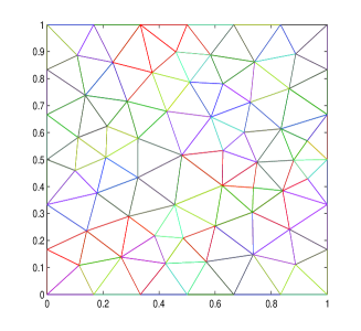
Figure 1: The initial mesh for the unit square.

In this example, the initial mesh $\mathcal{T}_{h_{1}}$ is showed in Figure 1 which is generated by Delaunay method and the mesh size $h_{1}=1/6$. Then we produce a sequence of meshes $\{\mathcal{T}_{h_{i}}\}_{i=2}^{6}$ which are obtained by the regular refinement (connecting the midpoints of each edge) and whose mesh sizes are $h_{2}=1/12,\ \cdots,\ h_{6}=1/192$. Based on this sequence of meshes, a sequence of linear conforming finite element space $\{V_{h_{i}}\}_{i=1}^{6}$ and $H(\mathrm{div};\Omega)$ conforming finite element space $\{\mathbf{W}_{h_{i}}^{1}\}_{i=1}^{6}$ are built.

First we solve the GPE problem (2.1) in $\{V_{h_{i}}\}_{i=1}^{6}$ and the dual problem (5.1) in $\{\mathbf{W}_{h_{i}}^{1}\}_{i=1}^{6}$, respectively. The corresponding numerical results are presented in Figure 2 which shows that the a posteriori error estimate $\eta(\lambda_{h},u_{h},\mathbf{p}_{h}^{*})$ is efficient when we solve the dual problem in $\mathbf{W}_{h}^{1}$. In Figure 2, we can find that the eigenvalue approximation $\lambda_{h}^{L}$ and ground state energy approximation $E_{h}^{L}$ are really asymptotic lower bounds for the first eigenvalue $\lambda$ and ground state energy $E$, respectively.

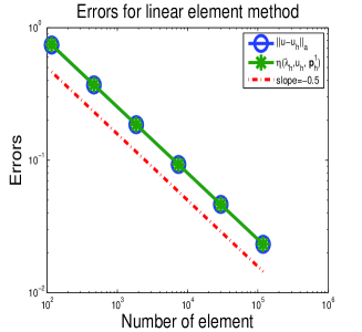
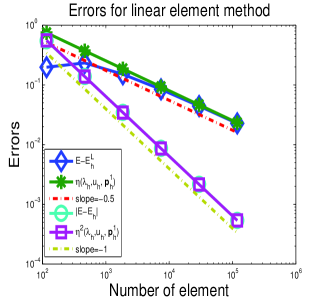
Figure 2: The errors for the unit square domain when the eigenvalue problem is solved by the linear finite element method, where $\eta(\lambda_{h},u_{h},\mathbf{p}_{h}^{1})$ denotes the a posteriori error estimates $\eta(\lambda_{h},u_{h},\mathbf{p}_{h}^{*})$ when the dual problem is solved in $\mathbf{W}_{h}^{1}$, and $\lambda_{h}^{L}$ denotes the asymptotic lower bound of the first eigenvalue and $E_{h}^{L}$ denotes the asymptotic lower bound of the ground state energy.

Example 5.2.

In this example, we solve the ground state solution of GPE (1.1) for BEC with $\zeta=1$, $W(x)=x_{1}^{2}+x_{2}^{2}$ on the L shape domain $\Omega=(-1,1)\times(-1,1)/[0,1)\times(-1,0]$.

Since $\Omega$ has a re-entrant corner, the singularity of the first eigenfunction is expected. The convergence order for the eigenvalue approximation is less than $2$ by the linear finite element method which is the order predicted by the theory for regular eigenfunctions. Since the exact eigenvalue is not known, we choose an adequately accurate approximation obtained by the higher order finite element and finer mesh as the exact first eigenpair for the numerical tests. In order to treat the singularity of the eigenfunction, we solve the GPE (2.1) by the adaptive finite element method (cf. [13, 20]).

We present this example to validate the results in this paper also hold on the adaptive meshes. In order to use the adaptive finite element method, we define the a posteriori error estimator as follows: Define the element residual $\mathcal{R}_{K}(\lambda_{h},u_{h})$ and the jump residual $\mathcal{J}_{E}(u_{h})$ as follows (see e.g., [20]):

$$\mathcal{R}_{K}(\lambda_{h},u_{h}) := \lambda_{h}u_{h}-\zeta|u_{h}|^{2}u_{h}-Wu_{h}+\Delta u_{h}\ \ \ {\rm in}\ K\in\mathcal{T}_{h},$$

$$\mathcal{J}_{E}(u_{h}) := -\nabla u_{h}^{+}\cdot\mathbf{\nu}^{+}-\nabla u_{h}^{-}\cdot\mathbf{\nu}^{-}:=[[\nabla u_{h}]]_{E}\cdot\mathbf{\nu}_{E},\ \ {\rm on}\ E\in\mathcal{E}_{h},$$

where $\mathcal{E}_{h}$ denotes the interior edge set in the mesh $\mathcal{T}_{h}$, $E$ is the common side of elements $K^{+}$ and $K^{-}$ with unit outward normals $\mathbf{\nu}^{+}$ and $\mathbf{\nu}^{-}$, respectively, and $\mathbf{\nu}_{E}=\mathbf{\nu}^{-}$.

For $K\in\mathcal{T}_{h}$, we define the local error indicator $\eta_{h}(\lambda_{h},u_{h},K)$ by

$$\eta_{h}^{2}(\lambda_{h},u_{h},K):=h_{K}^{2}\|\mathcal{R}_{K}(\lambda_{h},u_{h})\|_{0,K}^{2}+\sum_{E\in\mathcal{E}_{h},E\subset\partial K}h_{E}\|\mathcal{J}_{E}(u_{h})\|_{0,E}^{2}.$$ (5.2)

Then we define the global a posteriori error estimator $\eta_{ad}(\lambda_{h},u_{h})$ by

$$\eta_{ad}(\lambda_{h},u_{h}):=\left(\sum_{K\in\mathcal{T}_{h}}\eta_{h}^{2}(\lambda_{h},u_{h},K)\right)^{1/2}.$$ (5.3)

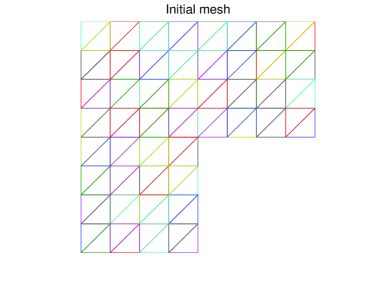
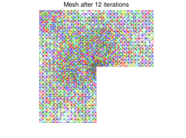
Figure 3: The initial mesh of L-shape domain (left) and the triangulation after 12 adaptive iterations for L-shape domain (right).

In this example, we solve (2.4) in the linear conforming finite element space $V_{h}$ and solve the dual problem (5.1) in the finite element space $\mathbf{W}_{h}^{1}$ , respectively. Figure 3 show the initial mesh (left) and corresponding adaptive mesh (right) after 15 iterations. The corresponding numerical results are presented in Figure 4 which shows that the a posteriori error estimate $\eta(\lambda_{h},u_{h},\mathbf{p}_{h}^{*})$ is also efficient even on the adaptive meshes when we solve the dual problem in $\mathbf{W}_{h}^{1}$. Figure 4 also shows the eigenvalue approximation $\lambda_{h}^{L}$ and ground state energy approximation $E_{h}^{L}$ are really asymptotic lower bounds for the first eigenvalue $\lambda$ and ground state energy $E$, respectively.

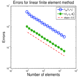
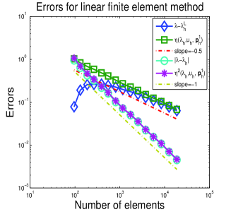
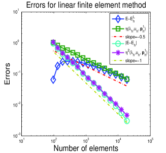
Figure 4: The errors for the L shape domain when the eigenvalue problem is solved by the linear finite element method, where $\eta(\lambda_{h},u_{h},\mathbf{p}_{h}^{1})$ denotes the a posteriori error estimates $\eta(\lambda_{h},u_{h},\mathbf{p}_{h}^{*})$ when the dual problem is solved in $\mathbf{W}_{h}^{1}$, and $\lambda_{h}^{L}$ denotes the asymptotic lower bounds of the first eigenvalue and $E_{h}^{L}$ denotes the asymptotic lower bound of the ground state energy.

6 Concluding remarks

In this paper, we give a computable error estimate for the eigenpair approximation by the general conforming finite element methods on general meshes. Furthermore, the asymptotic lower bound of the first eigenvalue and ground state energy can be obtained by the computable error estimate. Some numerical examples are provided to demonstrate the validation of the asymptotic lower bounds for he first eigenvalue and ground state energy. The method here can be extended to many other nonlinear eigenvalue problems, such as Kohn-Sham model for Schrödinger equation. Moreover, we can adopt the efficient numerical methods to obtain these lower bound, such as multilevel correction and multigrid method (cf. [35, 47, 48]).

From the definitions (4.3) and (4.7) and numerical examples, we can find the accuracy of lower bounds $\lambda_{h}^{L}$ and $E_{h}^{L}$ is not optimal. How to produce the lower bounds with optimal accuracy will be our future work.

References

- [1] R. A. Adams, Sobolev spaces, Academic Press, New York, 1975.
- [2] S. K. Adhikari, Collapse of attractive Bose-Einstein condensed vortex states in a cylindrical trap, Phys. Rev. E, 65 (2002), 016703.
- [3] S. K. Adhikari, P. Muruganandam, Bose-Einstein condensation dynamics from the numerical solution of the Gross-Pitaevskii equation, J. Phys. B, 35 (2002), 2831.
- [4] M. Ainsworth and J. Oden, A posteriori error estimation in finite element analysis, Pure and Applied Mathematics (New York), John Wiley & Sons, New York, 2000.
- [5] J. R. Anglin and W. Ketterle, Bose-Einstein condensation of atomic gasses, Nature, 416 (2002), 211-218
- [6] M. G. Armentano and R. G. Durán, Asymptotic lower bounds for eigenvalues by nonconforming finite element method, Electron. Trans. Numer. Anal., 17 (2004), 93-101.
- [7] I. Babuška and W. C. Rheinboldt, Error estimates for adaptive finite ele- ment computations, SIAM J. Numer. Anal., 15 (1978), 736-754.
- [8] I. Babuška and W. Rheinboldt, A-posteriori error estimates for the finite element method, Int. J. Numer. Methods Eng., 12 (1978), 1597-1615.
- [9] W. Bao, Y. Cai, Mathematical theory and numerical methods for Bose-Einstein condensation, Kinet. Relat. Models, 6(1) (2013), 1-135.
- [10] W. Bao, D. Jaksch and P.A. Markowich, Numerical solution of the Gross- Pitaevskii equation for Bose-Einstein condensation, J. Comput. Phys., 187(1) (2003), 318-342.
- [11] W. Bao, Shi Jin and P.A. Markowich, Numerical study of time-splitting spectral discretizations of nonlinear Schrödinger equations in the semi-classical regimes, SIAM J. Sci. Comput., 25(1) (2003), 27-64.
- [12] W. Bao and W. Tang, Ground-state solution of trapped interacting Bose-Einstein condensate by directly minimizing the energy functional, J. Comput. Phys., 187 (2003), 230-254.
- [13] S. Brenner and L. Scott, The Mathematical Theory of Finite Element Methods, New York: Springer-Verlag, 1994.
- [14] F. Brezzi and M. Fortin, Mixed and Hybrid Finite Element Methods, New York: Springer-Verlag, 1991.
- [15] E. Cancès, SCF algorithms for Hartree-Fock electronic calculations, Mathematical Models and Methods for Ab Initio Quantum Chemistry, Lecture Notes in Chemistry 74, Springer, Berlin, 2000.
- [16] E. Cancès, R. Chakir and Y. Maday, Numerical analysis of nonlinear eigenvalue problems, J. Sci. Comput., 45(1-3) (2010), 90-117.
- [17] C. Carstensen and D. Gallistl, Guaranteed lower eigenvalue bounds for the biharmonic equation, Numer. Math., 126 (2014), 33-51.
- [18] C. Carstensen and J. Gedicke, Guaranteed lower bounds for eigenvalues, Math. Comp., 83(290) (2014), 2605-2629.
- [19] M. M. Cerimele, M. L. Chiofalo, F. Pistella, S. Succi and M. P. Tosi, Numerical solution of the Gross-Pitaevskii equation using an explicit finite-difference scheme: an application to trapped Bose-Einstein condensates, Phys. Rev. E, 62 (2000), 1382.
- [20] H. Chen, L. He and A. Zhou, Finite element approximations of nonlinear eigenvalue problems in quantum physics, Comput. Methods Appl. Mech. Engrg., 200 (2011), 1846-1865.
- [21] P. G. Ciarlet, The Finite Element Method for Elliptic Problems, Amsterdam: North-Holland, 1978.
- [22] E. A. Cornell, Very cold indeed: the nanokelvin physics of Bose-Einstein condensation J. Res. Natl Inst. Stand., 101 (1996), 419-434.
- [23] F. Dalfovo, S. Giorgini, L. P. Pitaevskii and S. Stringari, Theory of Bose-Einstein condensation in trapped gases, Rev. Mod. Phys., 71 (1999), 463-512.
- [24] M. Edwards and K. Burnett, Numerical solution of the nonlinear Schrödinger equation for small samples of trapped neutral atoms, Phys. Rev. A, 51 (1995), 1382.
- [25] E. P. Gross, Nuovo, Cimento., 20 (1961), 454.
- [26] J. Haslinger and I. Hlaváček, Convergence of a finite element method based on the dual variational formulation, Apl. Mat., 21 (1976), 43-65.
- [27] L. V. Hau, B. D. Busch, C. Liu, Z. Dutton, M. M. Burns and J. A. Golovchenko, Near-resonant spatial images of confined Bose-Einstein condensates in a 4-Dee magnetic bottle, Phys. Rev. A, 58 (1998), R54-57.
- [28] J. Hu, Y. Huang and Q. Lin, The lower bounds for eigenvalues of elliptic operators by nonconforming finite element methods, J. Sci. Comput., 61(1) (2014), 196-221.
- [29] S. Jin, C. D. Levermore, and D. W. McLaughlin, The semiclassical limit of the Defocusing Nonlinear Schrödinger Hierarchy, CPAM, 52 (1999), 613-654.
- [30] L. Laudau and E. Lifschitz, Quantum Mechanics: non-relativistic theory, Pergamon Press, New York, 1977.
- [31] E. H. Lieb, R. Seiringer and J. Yangvason, Bosons in a trap: a rigorous derivation of the Gross-Pitaevskii energy functional, Phys. Rev. A, 61 (2000), 043602.
- [32] Q. Lin, F. Luo, H. Xie, A posterior error estimator and lower bound of a nonconforming finite element method, J. Comput. App. Math., 265 (2014), 243-254.
- [33] Q. Lin and H. Xie, The asymptotic lower bounds of eigenvalue problems by nonconforming finite element methods, Math. in Practice and Theory (in Chinese), 42(11) (2012), 219-226.
- [34] Q. Lin and H. Xie, Recent results on Lower bounds of eigenvalue problems by nonconforming finite element methods, Inverse Problems and Imaging, 7(3), 2013, 795-811.
- [35] Q. Lin and H. Xie, A multi-level correction scheme for eigenvalue problems, Math. Comp., 84(291) (2015), 71-88.
- [36] Q. Lin, H. Xie, F. Luo, Y. Li and Y. Yang, Stokes eigenvalue approximation from below with nonconforming mixed finite element methods, Math. in Practice and Theory (in Chinese), 19 (2010), 157-168.
- [37] X. Liu, A framework of verified eigenvalue bounds for self-adjoint differential operators, Appl. Math. Comput., 267 (2015), 341-355.
- [38] X. Liu and S. Oishi, Verifed eigenvalue evaluation for the Laplacian over polygonal domains of arbitrary shape, SIAM J. Numer. Anal., 51(3) (2013), 1634-1654.
- [39] F. Luo, Q. Lin, H. Xie, Computing the lower and upper bounds of Laplace eigenvalue problem: by combining conforming and nonconforming finite element methods, Sci. China Math., 55(5) (2012), 1069-1082.
- [40] P. Neittaanmäki and S. Repin, Reliable methods for computer simulation, Error control and a posteriori estimates, vol. 33 of Studies in Mathematics and its Applications, Elsevier Science B. V., Amsterdam, 2004.
- [41] S. Repin, A posteriori estimates for partial differential equations, vol. 4 of Radon Series on Computational and Applied Mathematics, Walter de Gruyter GmbH & Co. KG, Berlin, 2008.
- [42] B. I. Schneider, D. L. Feder, Numerical approach to the ground and excited states of a Bose-Einstein condensated gas confined in a completely anisotropic trap, Phys. Rev. A, 59 (1999), 2232.
- [43] I. Šebestová and T. Vejchodský, Two-sided bounds for eigenvalues of differential operators with applications to Friedrichs’, Poincaré, trace, and similar constants, SIAM J. Numer. Anal., 52(1) (2014), 308-329.
- [44] T. Vejchodský, Complementarity based a posteriori error estimates and their properties, Math. Comput. Simulation, 82 (2012), 2033-2046.
- [45] T. Vejchodský, Computing upper bounds on Friedrichs’ constant, in Applications of Mathematics 2012, J. Brandts, J. Chleboun, S. Korotov, K. Segeth, J. Šístek, and T. Vejchodský, eds., Institute of Mathematics, ASCR, Prague, 2012, pp. 278-289.
- [46] R. Verfürth, A review of a posteriori error estimation and adaptive mesh-refinement techniques, Wiley-Teubner, Chichester/Stuttgart, 1996.
- [47] H. Xie, A multigrid method for eigenvalue problem, J. Comput. Phys., 274 (2014), 550-561.
- [48] H. Xie and M. Xie, A Multigrid Method for the Ground State Solution of Bose-Einstein Condensates, Commun. Comput. Phys., 19(3) (2016), 648-662.
- [49] Y. Yang, Z. Zhang and F. Lin, Eigenvalue approximation from below using non-forming finite elements, Sci. China. Math., 53 (2010), 137-150.
- [50] Z. Zhang, Y. Yang and Z. Chen, Eigenvalue approximation from below by Wilson’s element, Chinese J. Numer. Math. Appl., 29 (2007), 81-84.
- [51] A. Zhou, An analysis of fnite-dimensional approximations for the ground state solution of Bose-Einstein condensates, Nonlinearity, 17 (2004), 541-550.