A Multigrid Method for the Ground State Solution of Bose-Einstein Condensates Based on Newton Iteration

Abstract

In this paper, a new kind of multigrid method is proposed for the ground state solution of Bose-Einstein condensates based on Newton iteration method. Instead of treating eigenvalue $\lambda$ and eigenvector $u$ respectively, we regard the eigenpair $(\lambda,u)$ as one element in the composite space $\mathbb{R}\times H_{0}^{1}(\Omega)$ and then Newton iteration method is adopted for the nonlinear problem. Thus in this multigrid scheme, we only need to solve a linear discrete boundary value problem in every refined space, which can improve the overall efficiency for the simulation of Bose-Einstein condensations. Keywords. BEC, GPE, nonlinear eigenvalue problem, multigrid method, finite element method. AMS subject classifications. 65N30, 65N25, 65L15, 65B99.

1 Introduction

A Bose-Einstein condensate (BEC) is a state of a dilute gas of bosons cooled to temperature very close to absolute zero. Under such condition, a large fraction of bosons will occupy the lowest quantum state, at which point, macroscopic quantum becomes apparent. BEC was first proposed by A. Einstein who generalized a work of S. N. Bose on the quantum statistics for photons [9] to a gas of non-interacting bosons [19, 20]. Then Gross-Pitaevskii theory was developed by Gross [21] and Pitaevskii [24] independently in 1960s to describe the dynamics of a BEC [25]. Since the first experimental observation of BEC in 1995, much attention has been paid to the Gross-Pitaevskii equation (GPE).

In the past decades, there have existed many papers discussing the numerical methods for the time-dependent GPEs and time-independent GPEs. Please refer to [2, 3, 5, 10, 11] and the papers cited therein. Especially, in [15, 28], the convergence and the priori error estimates of the finite element method for GPEs have been proved, which will be used later in this paper.

Solving such kind of nonlinear eigenvalue problem is an important but difficult problem in science and engineering computation. As is known to us all, the multigrid method provides an optimal complexity algorithm to solve discrete boundary value problems. The aim of this paper is to propose a multigrid scheme for GPEs based on Newton iteration method. More precisely, GPE is regarded as a nonlinear problem in the composite space $\mathbb{R}\times H_{0}^{1}(\Omega)$ and then Newton iteration is adopted to derive a linearized boundary value problem. Thus, we just need to solve a linear problem with finite element method in every refined space. With this multigrid scheme, solving GPE problem will not be more difficult than solving the corresponding boundary value problem. Besides, the convergence rate and computational work of this method are also analyzed in this paper.

An outline of the paper goes as follows. In Section 2, we introduce the finite element method and corresponding convergence estimates for the ground state solution of BEC, i.e. non-dimensionalized GPE. A Newton iteration method for GPE is presented in Section 3. In Section 4, we propose a type of multigrid algorithm for GPE based on Newton iteration method. Section 5 is devoted to estimating the computational work of the multigrid method designed in Section 4. Two numerical examples are presented in Section 6 to validate the theoretical analysis. Finally, some concluding remarks are given in the last section.

2 Finite element method for Gross-Pitaevskii equation

This section is devoted to introducing some notation and the finite element method for GPE problem. The letter $C$ (with or without subscripts) denotes a generic positive constant which may be different at its different occurrences. For convenience, the symbols $\lesssim$, $\gtrsim$ and $\approx$ will be used in this paper to denote $x_{1}\leq C_{1}y_{1}$, $x_{2}\geq c_{2}y_{2}$ and $c_{3}x_{3}\leq y_{3}\leq C_{3}x_{3}$ for some constants $C_{1},c_{2},c_{3}$, $C_{3}$ that are independent of mesh sizes (see, e.g., [27]). We shall use the standard notation for Sobolev spaces $W^{s,p}(\Omega)$ and their associated norms $\|\cdot\|_{s,p,\Omega}$ and seminorms $|\cdot|_{s,p,\Omega}$ (see, e.g., [1]). For $p=2$, we denote $H^{s}(\Omega)=W^{s,2}(\Omega)$, $H_{0}^{1}(\Omega)=\{v\in H^{1}(\Omega):\ v|_{\partial\Omega}=0\}$, where $v|_{\partial\Omega}=0$ is in the sense of trace and $\|\cdot\|_{s,\Omega}=\|\cdot\|_{s,2,\Omega}$. In this paper, we set $V=H_{0}^{1}(\Omega)$ and use $\|\cdot\|_{s}$ to denote $\|\cdot\|_{s,\Omega}$ for simplicity.

It is known that the wave function $\psi$ of a sufficiently dilute condensate, in the presence of an external potential $\widetilde{W,}$ satisfies the following GPE

$$\left(-\frac{\hbar^{2}}{2m}\Delta+\widetilde{W}+\frac{4\pi\hbar^{2}aN}{m}|\psi|^{2}\right)\psi = \mu\psi,$$ (2.1)

where $\mu$ is the chemical potential and $N$ is the number of atoms in the condensate, $4\pi\hbar^{2}a/m$ represents the effective two-body interaction, $\hbar$ is the Plank constant, $a$ is the scattering length (positive for repulsive interaction and negative for attractive interaction) and $m$ is the particle mass. In this paper, we assume the external potential $\widetilde{W}(x)$ is measurable, locally bounded and tends to infinity as $|x|\rightarrow\infty$ in the sense that

$$\inf_{|x|\geq r}\widetilde{W}(x)\rightarrow\infty\ \ \ \ {\rm as}\ r\rightarrow\infty.$$

Then the wave function $\psi$ must vanish exponentially fast as $|x|\rightarrow\infty$. Furthermore, (2.1) can be written as

$$\left(-\Delta+\frac{2m}{\hbar^{2}}\widetilde{W}+8\pi aN|\psi|^{2}\right)\psi = \frac{2m\mu}{\hbar^{2}}\psi.$$ (2.2)

Hence in this paper, we are concerned with the smallest eigenpair for the following non-dimensionalized GPE problem:

$$\left\{\begin{array}[]{rcl}-{\Delta}u+Wu+\zeta|u|^{2}u&=&\lambda u,\ \ \ {\rm in}\ \Omega,\\ u&=&0,\ \ \ \ \ {\rm on}\ \partial\Omega,\\ \int_{\Omega}|u|^{2}{d\Omega}&=&1,\end{array}\right.$$ (2.3)

where $\Omega\subset\mathbb{R}^{d}$ $(d=1,2,3)$ denotes the computing domain which has the cone property [1], $\zeta$ is some positive constant and $W(x)=\gamma_{1}x^{2}_{1}+\cdots+\gamma_{d}x^{2}_{d}\geq 0$ with $\gamma_{1},\cdots,\gamma_{d}>0$ [12, 28].

For the aim of finite element discretization, the corresponding weak form for (2.3) can be described as follows: Find $(\lambda,u)\in\mathbb{R}\times V$ such that $b(u,u)=1$ and

$$a(u,v)=\lambda b(u,v),\ \ \ \forall v\in V,$$ (2.4)

where

$$a(u,v)=\int_{\Omega}\big{(}\nabla u\cdot\nabla v+Wuv+\zeta|u|^{2}uv\big{)}d\Omega,\ \ \ \ b(u,v)=\int_{\Omega}uvd\Omega.$$

We also introduce the linearized form $a^{\prime}(u;v,w)$ by

$$a^{\prime}(u;v,w)=\int_{\Omega}\big{(}\nabla v\cdot\nabla w+Wvw+3\zeta|u|^{2}vw\big{)}d\Omega,\quad\forall v,w\in V.$$ (2.5)

Here and hereafter in this paper, we only consider the smallest eigenvalue and the corresponding eigenfunction of the problem (2.4). For GPE problem, we can find the following estimates from [15].

Lemma 2.1.

There exist positive constants $M,\ C_{L}$ and $C_{U}$ such that for all $v\in H_{0}^{1}(\Omega)$,

$$0\leq(\nabla v,\nabla v)+(Wv+\zeta|u|^{2}v,v)-\lambda(v,v)\leq M\|v\|_{1}^{2}$$ (2.6)

and

$$C_{L}\|v\|_{1}^{2}\leq a^{\prime}(u;v,v)-\lambda(v,v)\leq C_{U}\|v\|_{1}^{2}.$$ (2.7)

Now, let us define the finite element method [8, 17] for the problem (2.4). First we generate a shape-regular decomposition of the computing domain $\Omega\subset\mathbb{R}^{d}$ and the diameter of a cell $K\in\mathcal{T}_{h}$ is denoted by $h_{K}$. The mesh diameter $h$ describes the maximum diameter of all cells $K\in\mathcal{T}_{h}$. Based on the mesh $\mathcal{T}_{h}$, we construct the linear finite element space denoted by $V_{h}\subset V$. We assume that $V_{h}\subset V$ satisfies the following assumption:

$$\lim_{h\rightarrow 0}\inf_{v\in V_{h}}\|w-v\|_{1}=0,\ \ \ \forall w\in V.$$ (2.8)

The standard finite element method for (2.4) is to solve the following eigenvalue problem: Find $(\lambda_{h},u_{h})\in\mathbb{R}\times V_{h}$ such that $b(u_{h},u_{h})=1$ and

$$a(u_{h},v_{h})=\lambda_{h}b(u_{h},v_{h}),\ \ \ \forall v_{h}\in V_{h}.$$ (2.9)

Then we define

$$\delta_{h}(u):=\inf_{v_{h}\in V_{h}}\|u-v_{h}\|_{1}.$$ (2.10)

The convergence estimates of the finite element method for (2.4) are presented in the following lemma which can be found in [15, 28].

Lemma 2.2.

([15, Theorem 1]) There exists $h_{0}>0$, such that for all $0<h<h_{0}$, the smallest eigenpair approximation $(\lambda_{h},u_{h})$ of (2.9) has the following error estimates

$$\|u-u_{h}\|_{1} \lesssim \delta_{h}(u),$$ (2.11)

$$\|u-u_{h}\|_{0} \lesssim \eta_{a}(V_{h})\|u-u_{h}\|_{1}\lesssim\eta_{a}(V_{h})\delta_{h}(u),$$ (2.12)

$$|\lambda-\lambda_{h}| \lesssim \|u-u_{h}\|^{2}_{1}+\|u-u_{h}\|_{0}\lesssim\eta_{a}(V_{h})\delta_{h}(u),$$ (2.13)

where $\eta_{a}(V_{h})$ is defined as follows

$$\eta_{a}(V_{h})=\|u-u_{h}\|_{1}+\sup_{f\in L^{2}(\Omega),\|f\|_{0}=1}\inf_{v_{h}\in V_{h}}\|Tf-v_{h}\|_{1}$$ (2.14)

with the operator $T$ being defined as follows: Find $Tf\in u^{\perp}$ such that

$$a^{\prime}(u;Tf,v)-(\lambda(Tf),v)=(f,v),\ \ \ \ \forall v\in u^{\perp},$$

and $u^{\perp}=\big{\{}v\in H_{0}^{1}(\Omega)|\int_{\Omega}uvd\Omega=0\big{\}}$.

3 Newton iteration method for Gross-Pitaevskii equation

In this section, Newton iteration method is introduced to solve the GPE problem in a composite space defined as follows:

Denote the space $\mathbb{R}\times H_{0}^{1}(\Omega)$ by $X$ and $\mathbb{R}\times H^{-1}(\Omega)$ by $X^{*}$ with the norm

$$\|(\gamma,w)\|_{X}=|\gamma|+\|w\|_{1}\quad\text{and}\quad\|(\gamma,w)\|_{0}=|\gamma|+\|w\|_{0},\quad\forall(\gamma,w)\in X.$$

And the corresponding finite element space $\mathbb{R}\times V_{h}$ is denoted by $X_{h}$.

For any $(\gamma,w),\ (\mu,v)\in X$, we define a nonlinear operator $\mathcal{G}:X\rightarrow X^{*}$ as follows

$$\langle\mathcal{G}(\gamma,w),(\mu,v)\rangle = (\nabla w,\nabla v)+(Ww+\zeta|w|^{2}w-\gamma w,v)$$ (3.1)

$$\ \ \ +\frac{1}{2}\mu\left(1-\int_{\Omega}w^{2}d\Omega\right).$$

Since we request $\|u\|_{0}^{2}=1$, (2.4) can be rewritten as: Find $(\lambda,u)\in X$ such that

$$\langle\mathcal{G}(\lambda,u),(\mu,v)\rangle=0,\quad\forall(\mu,v)\in X.$$ (3.2)

The Fréchet derivation of $\mathcal{G}$ at $(\lambda,u)$ is given by

$$\langle\mathcal{G}^{\prime}(\lambda,u)(\gamma,w),(\mu,v)\rangle = (\nabla w,\nabla v)+((W+3\zeta u^{2}-\lambda)w,v)$$ (3.3)

$$\ \ \ -\gamma(u,v)-\mu(u,w)$$

$$= a^{\prime}(u;w,v)-\lambda(w,v)-\gamma(u,v)-\mu(u,w).$$

Assume we have an initial eigenpair approximation $(\lambda^{{}^{\prime}},u^{{}^{\prime}})$ on the finite element space $X_{h}$, Newton iteration method for GPE is defined as follows to get a better eigenpair approximation $(\lambda^{{}^{\prime\prime}},u^{{}^{\prime\prime}})\in X_{h}$:

$$\langle\mathcal{G}^{\prime}(\lambda^{{}^{\prime}},u^{{}^{\prime}})(\lambda^{{}^{\prime\prime}}-\lambda^{{}^{\prime}},u^{{}^{\prime\prime}}-u^{{}^{\prime}}),(\mu,v)\rangle=-\langle\mathcal{G}(\lambda^{{}^{\prime}},u^{{}^{\prime}}),(\mu,v)\rangle,\quad\forall(\mu,v)\in X_{h}.$$ (3.4)

From (3.1) and (3.3), (3.4) can be rewritten as follows: Find$(\lambda^{{}^{\prime\prime}},u^{{}^{\prime\prime}})\in X_{h}$, such that

$$\begin{cases}a(u^{{}^{\prime}};u^{{}^{\prime\prime}},v)-\lambda^{{}^{\prime\prime}}(u^{{}^{\prime}},v)=(2\zeta(u^{{}^{\prime}})^{3}-\lambda^{{}^{\prime}}u^{{}^{\prime}},v),\quad\forall v\in V_{h},\\ -\mu(u^{{}^{\prime}},u^{{}^{\prime\prime}})=-\mu/2-\mu(u^{{}^{\prime}},u^{{}^{\prime}})/2,\qquad\qquad\quad\ \ \forall\mu\in\mathbb{R}\end{cases}$$ (3.5)

with $a(u^{{}^{\prime}};u^{{}^{\prime\prime}},v)=a^{\prime}(u^{{}^{\prime}};u^{{}^{\prime\prime}},v)-\lambda^{{}^{\prime}}(u^{{}^{\prime\prime}},v)$.

The isomorphism property of $\mathcal{G}^{\prime}$ is analyzed in the following theorem.

Theorem 3.1.

If the mesh size $h$ is sufficiently small, then for the linearized operator $\mathcal{G}^{\prime}$ presented in (3.3), we have

$$\|(\gamma,w)\|_{X}\lesssim\mathop{\sup}\limits_{(\mu,v)\in X}\dfrac{\langle\mathcal{G}^{\prime}(\lambda,u)(\gamma,w),(\mu,v)\rangle}{\|(\mu,v)\|_{X}},\quad\forall(\gamma,w)\in X$$ (3.6)

and

$$\|(\gamma,w)\|_{X}\lesssim\mathop{\sup}\limits_{(\mu,v)\in X_{h}}\dfrac{\langle\mathcal{G}^{\prime}(\lambda,u)(\gamma,w),(\mu,v)\rangle}{\|(\mu,v)\|_{X}},\quad\forall(\gamma,w)\in X_{h}.$$ (3.7)

For any $(\hat{\lambda},\hat{u})\in X$ such that $\|(\hat{\lambda}-\lambda,\hat{u}-u)\|_{X}$ is small enough, there holds

$$\|(\gamma,w)\|_{X}\lesssim\mathop{\sup}\limits_{(\mu,v)\in X_{h}}\dfrac{\langle\mathcal{G}^{\prime}(\hat{\lambda},\hat{u})(\gamma,w),(\mu,v)\rangle}{\|(\mu,v)\|_{X}},\quad\forall(\gamma,w)\in X_{h}.$$ (3.8)

Proof.

For the first estimate (3.6), we just need to prove that the equation

$$\mathcal{G}^{\prime}(\lambda,u)(\gamma,w)=(\tau,f)$$ (3.9)

is uniquely solvable in $X$ for any $(\tau,f)\in X^{*}$. From (3.3), we obtain that (3.9) can be rewritten as

$$\begin{cases}a^{\prime}(u;w,v)-\lambda(w,v)+b_{u}(\gamma,v)=(f,v),\quad\forall v\in V,\\ b_{u}(\mu,w)=\mu\tau,\qquad\qquad\qquad\qquad\qquad~{}~{}~{}\quad\forall\mu\in\mathbb{R},\end{cases}$$

where $b_{u}(\mu,v)=-\mu(u,v)$.

For this saddle problem, the solvable condition is (Theorem 1.1 in [6], II):

Firstly, the following variational problem

$$a^{\prime}(u;w,v)-\lambda(w,v)=(f,v),\quad\forall v\in V_{0}$$ (3.10)

is uniquely solvable for any $f\in H^{-1}(\Omega)$ and $V_{0}:=\{v\in V:b_{u}(\mu,v)=0,\forall\mu\in\mathbb{R}\}$.

Secondly, $b_{u}(\cdot,\cdot)$ satisfies the inf-sup condition

$$\inf_{\mu\in\mathbb{R}}\sup_{v\in V}\dfrac{b_{u}(\mu,v)}{\|v\|_{1}|\mu|}\geq k_{b}$$ (3.11)

for some constant $k_{b}>0$.

The well-poseness of (3.10) can be derived from (2.7) directly.

For the second condition (3.11), take $v=-\mu u$. Since $\|u\|_{0}=1$, there holds

$$\inf_{\mu\in\mathbb{R}}\sup_{v\in V}\dfrac{b_{u}(\mu,v)}{\|v\|_{1}|\mu|}\geq\inf_{\mu\in\mathbb{R}}\dfrac{\mu^{2}(u,u)}{\|u\|_{1}|\mu|^{2}}=\frac{1}{\|u\|_{1}}=:k_{b}.$$

This completes the proof of (3.6).

From (2.7), we can define a project operator $P_{h}:V\rightarrow V_{h}$ by

$$a^{\prime}(u;w,v-P_{h}v)-\lambda(w,v-P_{h}v)=0,\quad\forall w\in V_{h},\ v\in V.$$ (3.12)

There apparently holds

$$\|P_{h}v\|_{1}\lesssim\|v\|_{1},\quad\forall v\in V.$$ (3.13)

From the Aubin-Nitsche lemma, we have

$$\|v-P_{h}v\|_{0}\lesssim\eta_{a}(V_{h})\|v\|_{1},\quad\forall v\in V.$$ (3.14)

So for any $(\gamma,w)\in X_{h}$, from (3.14), the following estimates hold

$$\|(\gamma,w)\|_{X} \lesssim \mathop{\sup}\limits_{(\mu,v)\in X}\dfrac{\langle\mathcal{G}^{\prime}(\lambda,u)(\gamma,w),(\mu,v)\rangle}{\|(\mu,v)\|_{X}}$$ (3.15)

$$= \mathop{\sup}\limits_{(\mu,v)\in X}\dfrac{\langle\mathcal{G}^{\prime}(\lambda,u)(\gamma,w),(\mu,P_{h}v)\rangle+\langle\mathcal{G}^{\prime}(\lambda,u)(\gamma,w),(0,v-P_{h}v)\rangle}{\|(\mu,v)\|_{X}}$$

$$= \mathop{\sup}\limits_{(\mu,v)\in X}\dfrac{\langle\mathcal{G}^{\prime}(\lambda,u)(\gamma,w),(\mu,P_{h}v)\rangle-\gamma(u,v-P_{h}v)}{\|(\mu,v)\|_{X}}$$

$$\lesssim \mathop{\sup}\limits_{(\mu,v)\in X}\dfrac{\langle\mathcal{G}^{\prime}(\lambda,u)(\gamma,w),(\mu,P_{h}v)\rangle+\gamma\|u\|_{0}\|v-P_{h}v\|_{0}}{\|(\mu,v)\|_{X}}$$

$$\lesssim \mathop{\sup}\limits_{(\mu,v)\in X}\dfrac{\langle\mathcal{G}^{\prime}(\lambda,u)(\gamma,w),(\mu,P_{h}v)\rangle+\gamma\eta_{a}(V_{h})\|u\|_{0}\|v\|_{1}}{\|(\mu,v)\|_{X}}$$

$$\lesssim \mathop{\sup}\limits_{(\mu,v)\in X}\dfrac{\langle\mathcal{G}^{\prime}(\lambda,u)(\gamma,w),(\mu,P_{h}v)\rangle}{\|(\mu,v)\|_{X}}+\eta_{a}(V_{h})\|(\gamma,w)\|_{X}.$$

Combing (3.13) and (3.15) leads to

$$\|(\gamma,w)\|_{X} \lesssim \mathop{\sup}\limits_{(\mu,v)\in X}\dfrac{\langle\mathcal{G}^{\prime}(\lambda,u)(\gamma,w),(\mu,P_{h}v)\rangle}{\|(\mu,v)\|_{X}}$$

$$\lesssim \mathop{\sup}\limits_{(\mu,v)\in X}\dfrac{\langle\mathcal{G}^{\prime}(\lambda,u)(\gamma,w),(\mu,P_{h}v)\rangle}{\|(\mu,P_{h}v)\|_{X}}$$

$$\lesssim \mathop{\sup}\limits_{(\mu,v)\in X_{h}}\dfrac{\langle\mathcal{G}^{\prime}(\lambda,u)(\gamma,w),(\mu,v)\rangle}{\|(\mu,v)\|_{X}}.$$

Then we get the desired conclusion (3.7).

For the last inequality (3.8), we assume there exists a sufficiently small constant $\varepsilon$ such that $\|(\hat{\lambda}-\lambda,\hat{u}-u)\|_{X}\leq\varepsilon$. Then for any $(\gamma,w)\in X_{h}$

$$\|(\gamma,w)\|_{X} \lesssim \mathop{\sup}\limits_{(\mu,v)\in X_{h}}\dfrac{\langle\mathcal{G}^{\prime}(\lambda,u)(\gamma,w),(\mu,v)\rangle}{\|(\mu,v)\|_{X}}$$

$$\lesssim \mathop{\sup}\limits_{(\mu,v)\in X_{h}}\dfrac{\langle\mathcal{G}^{\prime}(\hat{\lambda},\hat{u})(\gamma,w),(\mu,v)\rangle+\varepsilon\|(\gamma,w)\|_{X}\|(\mu,v)\|_{X}}{\|(\mu,v)\|_{X}}.$$

The desired result $(\ref{coercive of g3})$ then easily follows if $\varepsilon$ is sufficiently small. ∎

Applying Newton iteration method to GPE leads to a linearized problem, the corresponding residual estimate can be derived from the following theorem.

Theorem 3.2.

For the nonlinear operator $\mathcal{G}$ and any $(\mu_{h},v_{h}),(\mu,v)\in X$, we have

$$\langle\mathcal{G}(\mu_{h},v_{h}),(\sigma,\eta)\rangle = \langle\mathcal{G}(\mu,v),(\sigma,\eta)\rangle+\langle\mathcal{G}^{\prime}(\mu,v)(\mu_{h}-\mu,v_{h}-v),(\sigma,\eta)\rangle$$ (3.16)

$$+R\big{(}(\mu,v),(\mu_{h},v_{h}),(\sigma,\eta)\big{)},\quad\quad\forall(\sigma,\eta)\in X$$

with $R\big{(}(\mu,v),(\mu_{h},v_{h}),(\sigma,\eta)\big{)}$ being the residual which can be estimated as follows:

$$|R\big{(}(\mu,v),(\mu_{h},v_{h}),(\sigma,\eta)\big{)}|\lesssim\|(\mu-\mu_{h},v-v_{h})\|_{X}\|(\mu-\mu_{h},v-v_{h})\|_{0}\|(\sigma,\eta)\|_{X}.$$

Proof.

Define

$$\varphi(t)=\langle\mathcal{G}((\mu,v)+t(\mu_{h}-\mu,v_{h}-v)),(\sigma,\eta)\rangle.$$ (3.17)

Then the derivative of $\varphi$ with respect to $t$ can be derived trivially.

$$\varphi^{\prime}(t) = (\nabla(v_{h}-v),\nabla\eta)+(W(v_{h}-v),\eta)+3\big{(}\zeta(v+t(v_{h}-v))^{2}(v_{h}-v),\eta\big{)}$$

$$-(\mu_{h}-\mu)(v+t(v_{h}-v),\eta)-(\mu+t(\mu_{h}-\mu))(v_{h}-v,\eta)$$

$$-\sigma(v+t(v_{h}-v),v_{h}-v)$$

$$= \langle\mathcal{G}^{\prime}((\mu,v)+t(\mu_{h}-\mu,v_{h}-v))(\mu_{h}-\mu,v_{h}-v),(\sigma,\eta)\rangle$$

and

$$\varphi^{\prime\prime}(t) = -2(\mu_{h}-\mu)(v_{h}-v,\eta)-\sigma(v_{h}-v,v_{h}-v)$$ (3.18)

$$\ \ +6(\zeta(v+t(v_{h}-v))(v_{h}-v)^{2},\eta).$$

Denote $\xi=v+t(v_{h}-v)$ and from the imbedding theorem, we have

$$\|\xi\|_{0,6}\lesssim\|\xi\|_{1}\lesssim\|v\|_{1}+\|v_{h}\|_{1}.$$

For the last term of (3.18),

$$|(\xi(v_{h}-v)^{2},\eta)| \lesssim \int_{\Omega}|\xi|(v_{h}-v)^{2}|\eta|dx$$ (3.19)

$$\lesssim \|\xi\|_{0,6}\|v_{h}-v\|_{0}\|v_{h}-v\|_{0,6}\|\eta\|_{0,6}$$

$$\lesssim \|\xi\|_{1}\|v_{h}-v\|_{1}\|v_{h}-v\|_{0}\|\eta\|_{1}.$$

Thus, (3.16) can be derived from the following Taylor expansion

$$\varphi(1)=\varphi(0)+\varphi^{\prime}(0)+\int_{0}^{1}\varphi^{\prime\prime}(t)(1-t)dt.$$ (3.20)

Due to (3.18)-(3.20), the residual $R$ satisfies

$$|R\big{(}(\mu,v),(\mu_{h},v_{h}),(\sigma,\eta)\big{)}|\lesssim\|(\mu-\mu_{h},v-v_{h})\|_{X}\|(\mu-\mu_{h},v-v_{h})\|_{0}\|(\sigma,\eta)\|_{X}.$$

Then we complete the proof. ∎

4 Multigrid algorithm based on Newton iteration method

In this section, we propose a multigrid scheme based on Newton iteration method. In this algorithm, we only need to solve a linearized mixed variational problem on each refined finite element space.

4.1 One Newton iteration step

In order to design the multigrid method, we first introduce an one Newton iteration step in this subsection. Assume we have obtained an eigenpair approximation $(\lambda^{h_{k}},u^{h_{k}})\in\mathcal{R}\times V_{h_{k}}$, a type of iteration step will be introduced to derive an eigenpair $(\lambda^{h_{k+1}},u^{h_{k+1}})\in\mathcal{R}\times V_{h_{k+1}}$ with a better accuracy. In this paper, we denote by $(\lambda_{h_{k}},u_{h_{k}})$ the standard finite element solution of (2.4).

Algorithm 4.1.

One Newton Iteration Step

1. Define the linearized mixed variational equation on the finite element space $X_{h_{k+1}}$ as follows:

   Find $(\hat{\lambda}^{h_{k+1}},\hat{u}^{h_{k+1}})\in X_{h_{k+1}}$ such that for all $(\mu,v_{h_{k+1}})\in X_{h_{k+1}}$

   $$\begin{cases}a(u^{h_{k}};\hat{u}^{h_{k+1}},v_{h_{k+1}})-\hat{\lambda}^{h_{k+1}}(u^{h_{k}},v_{h_{k+1}})=(2\zeta(u^{h_{k}})^{3}-\lambda^{h_{k}}u^{h_{k}},v_{h_{k+1}}),\\ -\mu(\hat{u}^{h_{k+1}},u^{h_{k}})=-\mu/2-\mu(u^{h_{k}},u^{h_{k}})/2,\end{cases}$$ (4.1)

   where $a(u^{h_{k}};\hat{u}^{h_{k+1}},v_{h_{k+1}})=a^{\prime}(u^{h_{k}};\hat{u}^{h_{k+1}},v_{h_{k+1}})-\lambda^{h_{k}}(\hat{u}^{h_{k+1}},v_{h_{k+1}})$.

2. Solve equation $(\ref{one correction bvp})$ to obtain an eigenpair approximation $(\lambda^{h_{k+1}},u^{h_{k+1}})$ satisfying $\|(\lambda^{h_{k+1}}-\hat{\lambda}^{h_{k+1}},u^{h_{k+1}}-\hat{u}^{h_{k+1}})\|_{X}\lesssim\eta_{a}(V_{h_{k+1}})\delta_{h_{k+1}}(u)$.

In order to simplify the notation and summarize the above two steps, we define

$$(\lambda^{h_{k+1}},u^{h_{k+1}})=Newton_{-}Iteration(\lambda^{h_{k}},u^{h_{k}},V_{h_{k+1}}).$$

Theorem 4.1.

After implementing Algorithm 4.1, the resultant eigenpair approximation $(\lambda^{h_{k+1}},u^{h_{k+1}})$ has the following error estimate

$$\|(\lambda^{h_{k+1}}-\lambda_{h_{k+1}},u^{h_{k+1}}-u_{h_{k+1}})\|_{X}$$ (4.2)

$$\lesssim \eta_{a}(V_{h_{k+1}})\delta_{h_{k+1}}(u)+\delta_{h_{k}}(u)\|(\lambda_{h_{k}}-\lambda^{h_{k}},u_{h_{k}}-u^{h_{k}})\|_{X}$$

$$+\|(\lambda_{h_{k}}-\lambda^{h_{k}},u_{h_{k}}-u^{h_{k}})\|_{X}\|(\lambda_{h_{k}}-\lambda^{h_{k}},u_{h_{k}}-u^{h_{k}})\|_{0}.$$

Proof.

For the standard finite element solution $(\lambda_{h_{{k+1}}},u_{h_{{k+1}}})$, we have

$$\langle\mathcal{G}(\lambda_{h_{{k+1}}},u_{h_{{k+1}}}),(\mu,v_{h_{{k+1}}})\rangle=0,\quad\forall(\mu,v_{h_{{k+1}}})\in X_{h_{k+1}}.$$ (4.3)

Together with Theorem 3.2 and Algorithm 4.1, there holds

$$\langle\mathcal{G}^{\prime}(\lambda^{h_{k}},u^{h_{k}})(\lambda_{h_{k+1}}-\hat{\lambda}^{h_{k+1}},u_{h_{k+1}}-\hat{u}^{h_{k+1}}),(\mu,v_{h_{k+1}})\rangle$$

$$= \langle\mathcal{G}(\lambda^{h_{k}},u^{h_{k}}),(\mu,v_{h_{k+1}})\rangle$$

$$+\langle\mathcal{G}^{\prime}(\lambda^{h_{k}},u^{h_{k}})(\lambda_{h_{k+1}}-\lambda^{h_{k}},u_{h_{k+1}}-u^{h_{k}}),(\mu,v_{h_{k+1}})\rangle$$

$$= \langle\mathcal{G}(\lambda^{h_{k}},u^{h_{k}}),(\mu,v_{h_{k+1}})\rangle-\langle\mathcal{G}(\lambda_{h_{k+1}},u_{h_{k+1}}),(\mu,v_{h_{k+1}})\rangle$$

$$+\langle\mathcal{G}^{\prime}(\lambda^{h_{k}},u^{h_{k}})(\lambda_{h_{k+1}}-\lambda^{h_{k}},u_{h_{k+1}}-u^{h_{k}}),(\mu,v_{h_{k+1}})\rangle$$

$$= -R\big{(}(\lambda^{h_{k}},u^{h_{k}}),(\lambda_{h_{k+1}},u_{h_{k+1}}),(\mu,v_{h_{k+1}})\big{)}.$$

Using (3.8) and Theorem 3.2, we derive

$$\|(\lambda_{h_{k+1}}-\hat{\lambda}^{h_{k+1}},u_{h_{k+1}}-\hat{u}^{h_{k+1}})\|_{X}$$ (4.4)

$$\lesssim \|(\lambda_{h_{k+1}}-\lambda^{h_{k}},u_{h_{k+1}}-u^{h_{k}})\|_{X}\|(\lambda_{h_{k+1}}-\lambda^{h_{k}},u_{h_{k+1}}-u^{h_{k}})\|_{0}$$

$$\lesssim \eta_{a}(V_{h_{k}})\delta_{h_{k}}^{2}(u)+\delta_{h_{k}}(u)\|(\lambda_{h_{k}}-\lambda^{h_{k}},u_{h_{k}}-u^{h_{k}})\|_{X}$$

$$+\|(\lambda_{h_{k}}-\lambda^{h_{k}},u_{h_{k}}-u^{h_{k}})\|_{X}\|(\lambda_{h_{k}}-\lambda^{h_{k}},u_{h_{k}}-u^{h_{k}})\|_{0}.$$

Since

$$\|(\lambda^{h_{k+1}}-\hat{\lambda}^{h_{k+1}},u^{h_{k+1}}-\hat{u}^{h_{k+1}})\|_{X}\lesssim\eta_{a}(V_{h_{k+1}})\delta_{h_{k+1}}(u),$$

we arrive at

$$\|(\lambda^{h_{k+1}}-\lambda_{h_{k+1}},u^{h_{k+1}}-u_{h_{k+1}})\|_{X}$$

$$\lesssim \eta_{a}(V_{h_{k+1}})\delta_{h_{k+1}}(u)+\delta_{h_{k}}(u)\|(\lambda_{h_{k}}-\lambda^{h_{k}},u_{h_{k}}-u^{h_{k}})\|_{X}$$

$$+\|(\lambda_{h_{k}}-\lambda^{h_{k}},u_{h_{k}}-u^{h_{k}})\|_{X}\|(\lambda_{h_{k}}-\lambda^{h_{k}},u_{h_{k}}-u^{h_{k}})\|_{0}..$$

This completes the proof. ∎

4.2 Multigrid method

In order to do multigrid iteration, we define a sequence of triangulations $\mathcal{T}_{h_{k}}$ and $\mathcal{T}_{h_{k+1}}$ is produced from $\mathcal{T}_{h_{k}}$ via a regular refinement (produce $\beta^{d}$ congruent elements) such that

$$h_{k}\approx\frac{1}{\beta}h_{k-1},$$ (4.5)

where the integer $\beta$ denotes the refinement index and larger than $1$ (always equals $2$). Based on the mesh sequence, we construct a sequence of linear finite element spaces satisfying

$$V_{h_{1}}\subset V_{h_{2}}\subset\cdots\subset V_{h_{n}}\subset V$$ (4.6)

and assume the following relations of approximation errors hold

$$\eta_{a}(V_{h_{k}})\approx\frac{1}{\beta}\eta_{a}(V_{h_{k-1}}),\quad\delta_{h_{k}}(u)\approx\frac{1}{\beta}\delta_{h_{k-1}}(u),\ \ \ k=1,2,\cdots,n.$$ (4.7)

Obviously, the following relationship is also valid

$$X_{h_{1}}\subset X_{h_{2}}\subset\cdots\subset X_{h_{n}}\subset X.$$ (4.8)

The multigrid method based on one Newton iteration step is proposed in the following algorithm.

Algorithm 4.2.

Multigrid Algorithm

1. Construct a series of nested finite element spaces $V_{h_{1}},V_{h_{2}},\cdots,V_{h_{n}}$ such that $(\ref{mesh relationship})$ and $(\ref{delta_recur_relation})$ hold.

2. Solve the GPE on the initial finite element space $X_{h_{1}}$: Find $(\lambda^{h_{1}},u^{h_{1}})\in X_{h_{1}}$ such that

   $$(\nabla u^{h_{1}},\nabla v_{h_{1}})+(Wu^{h_{1}},v_{h_{1}})+(\zeta(u^{h_{1}})^{3},v_{h_{1}})=\lambda^{h_{1}}(u^{h_{1}},v_{h_{1}}),\quad\forall v\in V_{h_{1}}.$$

3. Do $k=1,\cdots,n-1$
   Obtain a new eigenpair approximation $(\lambda^{h_{k+1}},u^{h_{k+1}})$ by a Newton iteration step

   $$(\lambda^{h_{k+1}},u^{h_{k+1}})=Newton_{-}Iteration(\lambda^{h_{k}},u^{h_{k}},V_{h_{k+1}}).$$ (4.9)

   End Do.

Theorem 4.2.

Assume the initial mesh size $h_{1}$ is sufficiently small, after implementing Algorithm 4.2, the resultant eigenpair approximation $(\lambda^{h_{n}},u^{h_{n}})$ has the following error estimate

$$\|(\lambda_{h_{n}}-\lambda^{h_{n}},u_{h_{n}}-u^{h_{n}})\|_{X} \lesssim \eta_{a}(V_{h_{n}})\delta_{h_{n}}(u).$$ (4.10)

Proof.

From the second step of Algorithm 4.2, we have

$$0=\|(\lambda_{h_{1}}-\lambda^{h_{1}},u_{h_{1}}-u^{h_{1}})\|_{X} \lesssim \eta_{a}(V_{h_{1}})\delta_{h_{1}}(u).$$ (4.11)

Using Theorem 4.1, we derive

$$\|(\lambda_{h_{n}}-\hat{\lambda}^{h_{n}},u_{h_{n}}-\hat{u}^{h_{n}})\|_{X}$$ (4.12)

$$\lesssim \|(\lambda_{h_{n}}-\lambda^{h_{n-1}},u_{h_{n}}-u^{h_{n-1}})\|_{X}\|(\lambda_{h_{n}}-\lambda^{h_{n-1}},u_{h_{n}}-u^{h_{n-1}})\|_{0}$$

$$\lesssim \eta_{a}(V_{h_{n}})\delta_{h_{n}}(u)+\delta_{h_{n-1}}(u)\|(\lambda_{h_{n-1}}-\lambda^{h_{n-1}},u_{h_{n-1}}-u^{h_{n-1}})\|_{X}$$

$$\hskip-28.45274pt+\|(\lambda_{h_{n-1}}-\lambda^{h_{n-1}},u_{h_{n-1}}-u^{h_{n-1}})\|_{X}\|(\lambda_{h_{n-1}}-\lambda^{h_{n-1}},u_{h_{n-1}}-u^{h_{n-1}})\|_{0}.$$

Inequality (4.11) means that (4.10) holds for the initial finite element space $X_{h_{1}}$. Assume that (4.10) is true for the space $V_{h_{n-1}}$, i.e.,

$$\|(\lambda_{h_{n-1}}-\lambda^{h_{n-1}},u_{h_{n-1}}-u^{h_{n-1}})\|_{X}\lesssim\eta_{a}(V_{h_{n-1}})\delta_{h_{n-1}}(u).$$ (4.13)

Combining (4.12) and (4.13) leads to

$$\|(\lambda_{h_{n}}-\hat{\lambda}^{h_{n}},u_{h_{n}}-\hat{u}^{h_{n}})\|_{X}\lesssim\eta_{a}(V_{h_{n}})\delta_{h_{n}}(u).$$

Since

$$\|(\lambda^{h_{n}}-\hat{\lambda}^{h_{n}},u^{h_{n}}-\hat{u}^{h_{n}})\|_{X}\lesssim\eta_{a}(V_{h_{n}})\delta_{h_{n}}(u),$$

we arrive at

$$\|(\lambda^{h_{n}}-\lambda_{h_{n}},u^{h_{n}}-u_{h_{n}})\|_{X}\lesssim\eta_{a}(V_{h_{n}})\delta_{h_{n}}(u).$$

This completes the proof. ∎

Theorem 4.3.

For Algorithm 4.2, under the conditions of Thoerem 4.2, we have

$$\|(\lambda-\lambda^{h_{n}},u-u^{h_{n}})\|_{X} \lesssim \delta_{h_{n}}(u),$$ (4.14)

$$\|(\lambda-\lambda^{h_{n}},u-u^{h_{n}})\|_{0} \lesssim \eta_{a}(V_{h_{n}})\delta_{h_{n}}(u).$$ (4.15)

Proof.

Theorem 4.3 can be derived from Lemma 2.2, Theorem 4.2 and triangle inequality. ∎

5 Work estimate of multigrid algorithm

In this section, the computational work of Algorithm 4.2 is presented to show the efficiency of this multigrid scheme. Denote the dimension of finite element space $X_{h_{k}}$ by $N_{k}$. Then we have

$$N_{k}\approx\beta^{d(k-n)}N_{n},\ \ \ k=1,2,\cdots,n.$$

Theorem 5.1.

Assume the work of GPE problem in the initial finite element space $X_{h_{1}}$ is $\mathcal{O}(M_{h_{1}})$ and that of the linear boundary value problem in each level $X_{h_{k}}$ is $\mathcal{O}(N_{k})$ for $k=1,2,\cdots,n$. Then the work involved in the multigrid method is $\mathcal{O}(N_{n}+M_{h_{1}})$. Furthermore, the complexity can be $\mathcal{O}(N_{n})$ provided $M_{h_{1}}\leq N_{n}$.

Proof.

Denote the work in the $k-th$ finite element space $X_{h_{k}}$ by $W_{k}$ and the total work by $W$. Then

$$W = \sum_{k=1}^{n}W_{k}=\mathcal{O}(M_{h_{1}}+\sum_{k=2}^{n}N_{k})$$

$$= \mathcal{O}(M_{h_{1}}+\sum_{k=2}^{n}\beta^{d(k-n)}N_{n})$$

$$= \mathcal{O}(M_{h_{1}}+N_{n}).$$

Then we derive the desired result and $W=\mathcal{O}(N_{n})$ when $M_{h_{1}}\leq N_{n}$. ∎

6 Numerical results

In this section, two numerical examples are presented to illustrate the efficiency of the multigrid scheme proposed in this paper.

6.1 Example 1

In the first example, we use Algorithm 4.2 to solve the following GPE: Find $(\lambda,u)$ such that

$$\left\{\begin{array}[]{rcl}-\triangle u+Wu+\zeta|u|^{2}u&=&\lambda u,\quad{\rm in}\ \Omega,\\ u&=&0,\ \ \quad{\rm on}\ \partial\Omega,\\ \int_{\Omega}u^{2}d\Omega&=&1,\end{array}\right.$$ (6.1)

where $\Omega$ denotes the three dimensional domain $(0,1)^{3}$, $\zeta=1$ and $W=x_{1}^{2}+x_{2}^{2}+x_{3}^{2}$.

The sequence of finite element spaces are constructed by linear element on a series of meshes produced by regular refinement with $\beta=2$ (producing $\beta^{3}$ congruent subelements). Since the exact solution is not known, an adequate accurate approximation is choosen as the exact solution to investigate the convergence behavior. The optimal error estimates can be obtained from the numerical results which are presented in Figure 1.

In order to show the efficiency of Algorithm 4.2, we also provide the running time of Algorithm 4.2. Here, all schemes are running on the same machine PowerEdge R720 with the linux system hereafter. The corresponding results are presented in Table 1 and Figure 1, which imply the efficiency and linear complexity of Algorithm 4.2.

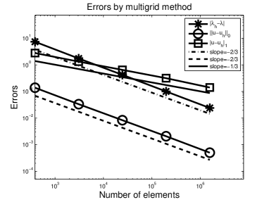
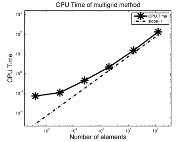
Figure 1: Left: The errors of the multigrid method for the ground state solution of GPE, where $\lambda_{h}$ and $u_{h}$ denote the numerical solutions of Algorithm 4.2. Right: CPU Time of Algorithm 4.2 for Example 1.

Table 1: The CPU time of Algorithm 4.2 for Example 1.

Number of levels	Number of elements	Time for Algorithm 4.2
1	3072	0.1089
2	24576	0.5249
3	196608	2.1467
4	1572846	15.7916
5	12582912	131.3590

6.2 Example 2

In the second example, we consider the GPE (6.1) on the domain $\Omega=(0,1)^{3}$ with the coefficient $\zeta=100$ and $W=x_{1}^{2}+2x_{2}^{2}+4x_{3}^{2}$. Numerical results are presented in Table 2 and Figure 2. Hence the efficiency and linear complexity of Algorithm 4.2 can also be validated.

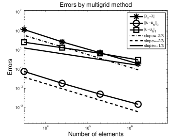
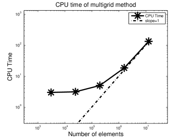
Figure 2: Left: The errors of the multigrid method for the ground state solution of GPE, where $\lambda_{h}$ and $u_{h}$ denote the numerical solutions of Algorithm 4.2. Right: CPU Time of Algorithm 4.2 for Example 2.

Table 2: The CPU time of Algorithm 4.2 for Example 2.

Number of levels	Number of elements	Time of Algorithm 4.2
1	24576	2.4686
2	196608	4.8973
3	1572846	18.3522
4	12582912	138.0450

7 Concluding remarks

In this paper, we propose a type of multigrid method for GPE problems based on Newton iteration. Different from the classical finite element method for GPE problems, the proposed method transforms the nonlinear eigenvalue problem solving to a series of linear boundary value problems solving and a eigenvalue problem solving in the coarsest finite element space. The high efficiency of linear boundary value problems solving can improve the overall efficiency of the simulation for BEC. The corresponding analysis about the computational complexity has also been given. The idea proposed here can also be extend to other nonlinear eigenvalue problems, i.e., Kohn-Sham equation, which always arises from the electronic structure computation.

References

• [1] R. A. Adams, Sobolev spaces, Academic Press, New York, 1975.
• [2] S. K. Adhikari, Collapse of attractive Bose-Einstein condensed vortex states in a cylindrical trap, Phys. Rev. E, 65 (2002), 016703.
• [3] S. K. Adhikari and P. Muruganandam, Bose-Einstein condensation dynamics from the numerical solution of the Gross-Pitaevskii equation, J. Phys. B, 35 (2002), 2831-2843.
• [4] M. H. Anderson, J. R. Ensher, M. R. Mattews, C. E. Wieman and E. A. Cornell, Observation of Bose-Einstein condensation in a dilute atomic vapor, Science, 269 (1995), 198-201.
• [5] J. R. Anglin and W. Ketterle, Bose-Einstein condensation of atomic gasses, Nature, 416 (2002), 211-218.
• [6] F. Brezzi and F. Fortin, Mixed and Hybrid Finite Element Methods, New York: Springer-Verlag, 1991.
• [7] J. H. Bramble and J. E. Pasciak, New convergence estimates for multigrid algorithms, Math. Comp., 49 (1987), 311-329.
• [8] S. Brenner and L. Scott, The Mathematical Theory of Finite Element Methods, New York: Springer-Verlag, 1994.
• [9] S. N. Bose, Plancks gesetz und lichtquantenhypothese, Zeitschrift für Physik, 3(1924), 178-181.
• [10] W. Bao and Y. Cai, Mathematical theory and numerical methods for Bose-Einstein condensation, Kinet. Relat. Models, 6(1) (2013), 1-135.
• [11] W. Bao and Q. Du, Computing the ground state solution of Bose–Einstein condensates by a normalized gradient flow, SIAM J. Sci. Comput., 25(5) (2004), 1674-1697.
• [12] W. Bao and W. Tang, Ground-state solution of trapped interacting Bose-Einstein condensate by directly minimizing the energy functional, J. Comput. Phys., 187(2003), 230-254.
• [13] E. A. Cornell, Very cold indeed: the nanokelvin physics of Bose-Einstein condensation, J. Res. Natl Inst. Stand., 101 (1996), 419-434.
• [14] E. A. Cornell and C. E. Wieman, Nobel Lecture: Bose-Einstein condensation in a dilute gas, the first 70 years and some recent experiments, Rev. Mod. Phys., 74 (2002), 875-893.
• [15] E. Cancès, R. Chakir and Y. Maday, Numerical analysis of nonlinear eigenvalue problems, J. Sci. Comput., 45(1-3) (2010), 90-117.
• [16] H. Chen, L. He and A. Zhou, Finite element approximations of nonlinear eigenvalue problems in quantum physics, Comput. Methods Appl. Mech. Engrg., 200(21) (2011), 1846-1865.
• [17] P. G. Ciarlet, The Finite Element Method for Elliptic Problems, Amsterdam: North-Holland, 1978.
• [18] F. Dalfovo, S. Giorgini, L. P. Pitaevskii and S. Stringari, Theory of Bose-Einstein condensation in trapped gases, Rev. Mod. Phys., 71 (1999), 463-512.
• [19] A. Einstein, Quantentheorie des einatomigen idealen gases, Sitzungsberichte der Preussis-chen Akademie der Wissenschaften, 22 (1924), 261-267.
• [20] A. Einstein, Quantentheorie des einatomigen idealen gases, zweite abhandlung, Sitzungs-berichte der Preussischen Akademie der Wissenschaften, 1 (1925), 3-14.
• [21] E. P. Gross, Structure of a quantized vortex in boson systems, Nuovo. Cimento., 20 (1961), 454-457.
• [22] L. Laudau and E. Lifschitz, Quantum Mechanics: non-relativistic theory, Pergamon Press, New York, 1977.
• [23] Q. Lin and H. Xie, A multi-level correction scheme for eigenvalue problems, Math. Comp., 84(291) (2015), 71-88.
• [24] L. P. Pitaevskii, Vortex lines in an imperfect Bose gas, Soviet Phys. JETP, 13 (1961), 451-454.
• [25] L. P. Pitaevskii and S. Stringari, Bose-einstein condensation, Oxford University Press, 2003.
• [26] H. Xie, A multigrid method for eigenvalue problem, J. Comput. Phys., 274 (2014), 550-561.
• [27] J. Xu, Iterative methods by space decomposition and subspace correction, SIAM Review, 34(4) (1992), 581-613.
• [28] A. Zhou, An analysis of fnite-dimensional approximations for the ground state solution of Bose-Einstein condensates, Nonlinearity, 17 (2004), 541-550.
• [29] O. Zienkiewicz and J. Zhu, The superconvergent patch recovery and a posteriori error estimates. Part 1: The recovery technique, Internat. J. Numer. Methods Engrg., 33(7) (1992), 1331-1364.