Finite-length scaling based on belief propagation
for spatially coupled LDPC codes

Abstract

The equivalence of peeling decoding (PD) and Belief Propagation (BP) for low-density parity-check (LDPC) codes over the binary erasure channel is analyzed. Modifying the scheduling for PD, it is shown that exactly the same variable nodes are resolved in every iteration than with BP. The decrease of erased VNs during the decoding process is analyzed instead of resolvable equations. This quantity can also be derived with density evolution, resulting in a drastic decrease in complexity. Finally, a scaling law using this quantity is established for spatially coupled LDPC codes.

I Introduction

Recently, it was shown that spatially-coupled low-density parity-check (SC-LDPC) codes can achieve the channel capacity of binary-input memoryless symmetric (BMS) channels under BP decoding [1, 2]. The Tanner graph of a block code with $M$ VNs, referred to as the uncoupled LDPC code graph, is duplicated $L$ times to produce a sequence of identical graphs, where $L$ is the chain length of the SC-LDPC code. The different copies are connected to form a chain by redirecting (spreading) certain edges. The asymptotic analysis of SC-LDPC code ensembles shows that they exhibit a BP threshold close to the maximum-a-posteriori (MAP) threshold of the uncoupled LDPC code ensemble for sufficiently large $L$ [3]. In addition, SC-LDPC code ensembles can be designed with a linear growth of the minimum distance with $M$ [4]. Indeed, the minimum distance growth rate for the coupled LDPC ensemble is often better than for the uncoupled ensemble [5]. Several families of SC-LDPC code ensembles are compared in [5, 6] using asymptotic arguments, namely BP threshold and minimum distance growth rate.

The performance of finite-length LDPC codes over a binary erasure channel (BEC) using a BP decoder is analyzed in [7, 8] by studying an alternative decoder, namely PD. Following this approach, the finite-length performance of SC-LDPC code ensembles over the BEC has recently been analyzed in [9, 10]. To the authors knowledge, the single attempt to generalize the PD-based finite-length analysis to a general message passing BP decoder is due to Ezri, Montanari and Urbanke in [11, 12], where scaling laws are conjectured for $(l,r)$-regular LDPC ensembles for the binary additive white Gaussian noise (BIAWGN) channel and scaling parameters are derived from the correlation of messages sent within the decoder. However, applying this analysis to SC-LDPC codes is prohibitively complex.

In this work, we present a finite-length analysis approach based on BP similar to the one base on PD in [8]. After showing the equivalence of BP and a particular form of PD with modified scheduling, we replace the analyzed random process used to predict the probability of a decoding failure and examine the decrease of erased VNs per iteration during the decoding process. We show that our approach predicts the waterfall performance correctly. Our substitute can also be derived from BP density evolution (DE), which has significantly lower complexity than graph evolution for PD.

After introducing parallel peeling decoding (PPD), its equivalence to BP is shown and we derive a graph evolution for PPD applied to protograph-based SC-LDPC codes. The properties shown in [10] are discussed using PPD. We then introduce and analyze the decrease of unresolved VNs per iteration and compare it with the number of resolvable check nodes available in each iteration. Finally, we establish a scaling law based on the decrease of unresolved VNs and verify the results with simulations.

This paper is structured as follows. Section II introduces construction and notation. In Section III, we introduce a modified form of PD called PPD and BP and discuss their equivalence. After deriving the graph evolution for PPD, we show exemplary that properties and differences between code ensembles observed with standard PD can still be observed from PPD. The analysis of the decoding trajectory based on resolved VNs per iteration for PPD and BP is discussed in Section IV. In Section V, we establish a scaling law based on this random process.

II SC-LDPC Code Constructions

We introduce two types of constructions, randomly constructed regular codes as proposed in [1, 9], and a construction based on protographs [10]. After defining the BEC, we define the residual graph degree distribution after transmission.

We denote vectors and matrices with $\mathbf{v}=(v_{1},v_{2},\dots,v_{n})$ and $\mathbf{M}$, respectively. Extending the notation for unit vectors, $\mathbf{e}_{i,j,k}$ is a vector where all entries are zero except the entries at positions $i$,$j$, and $k$ which are $1$, whereas $\mathbf{1}$ denotes a vector where all entries are ones. We also define $\mathbf{a}^{\mathbf{v}}=a_{1}^{v_{1}}a_{2}^{v_{2}}\dots$, where the exponent is set to $0$ for any $v_{i}\leq 0$. $|\mathbf{v}|=\sum_{i=1}^{n}v_{i}$ as $L^{1}$ norm is the sum of all entries of $\mathbf{v}$. Denote by $X=(X_{1},\dots,X_{n})$ a vector of $n$ random variables.

The message passed from CN $c$ to VN $v$ in iteration $\ell$ is denoted with $\mu_{{c}\rightarrow{v}}(\ell)$. We denote the set of VNs (CNs) connected to a specific CN $c$ (VN $v$) with $\mathcal{N}_{c}$ ($\mathcal{N}_{v}$).

Randomly Constructed ${(l,r,L)}_{u}$ SC-LDPC Codes

Let there be $L$ uncoupled $(l,r)$ regular LDPC codes where $l$ is the VN degree and $r$ is the CN degree, $r\leq l$, $\tfrac{l}{r}\in\mathbb{N}$. Each of the $L$ $(l,r)$ regular LDPC codes has $M$ VNs and $\tfrac{l}{r}M$ CNs and the codes are placed at $L$ consecutive positions. The ${(l,r,L)}_{u}$ code is obtained by spreading $l$ edges of each VN along consecutive positions, so that each VN at position $u$ is connected to a CN at positions $u,\dots,u+l-1$ and a chain of connected codes is obtained as depicted with an example in Fig. 1. When the CNs at each position are chosen at random, their maximum degree is fixed to $r$. However, there is randomness in the number of connections to VNs of a specific position. Note that there are $(l-1)$ additional positions at the end of the chain of coupled codes without any VNs but with CNs connected to VNs of codes on previous positions of the chain. For large $L$, the code rate tends to $\mathtt{r}_{{(l,r,L)}_{u}}=1-\tfrac{l}{r}$.

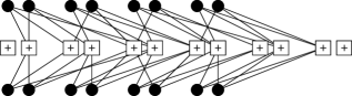
Figure 1: Construction of the ${(l,r,L)}_{u}=(3,6,4)_{u}$ coupled protograph with $M=4$ VNs per code. The CNs at positions $3$ and $4$ are regular and have degree $r=6$.

Protograph-based ${(l,r,L)}$ SC-LDPC Codes

The protographs as proposed by Thorpe in [13] are first copied $N$ times before edges of the same type are permuted to avoid small cycles in the resulting code. Such a protograph can be represented compactly by its bi-adjacency matrix $\mathbf{B}$, called the base matrix. Every $1$ in $\mathbf{B}$ is replaced by an $N\times N$ permutation matrix. With $v$ VNs in the protograph, $M=Nv$ VNs are obtained. All possible matrices $\mathbf{H}$ derived from all possible combinations of $N\times N$ permutation matrices give a code ensemble. The design rate $\mathtt{r}$ of this code ensemble can be directly computed from the protograph since the Tanner graph of $\mathbf{H}$ inherits the degree distribution (DD) and graph neighborhood structure of the protograph.

Figure 2: Construction of the ${(l,r,L)}=(3,6,3)$ coupled protograph.

We couple $(l,r)$-regular LDPC codes according to [3] with $\frac{r}{l}=k\in\mathbb{N}$. $L$ protographs are then connected to an $(l,r,L)$ coupled protograph by connecting each VN at position $u$, $1\leq u\leq L$ to the CNs at positions $u,\dots,u+l-1$ as shown in Fig. 2 for $L=3$. Each uncoupled protograph has $v=k$ VNs and one CN so that we obtain $M=2N$ VNs per coupled code after lifting the construction. We obtain a code length $\mathtt{n}=kLN$ bits and obtain a code rate of $\mathtt{r}_{(l,r,L)}=1-\tfrac{(L+l-1)}{kL}$.

II-A The Binary Erasure Channel

Denote by $X(t)\in\{0,1\}$ the binary channel input at a discrete time $t$ and the corresponding channel output $Y(t)\in\{0,1,\Delta\}$ where $\Delta$ denotes an erasure. We drop the indices for time where possible and use $s$ if $Y\in\{0,1\}$ is known and solved. A symbol is erased during transmission with probability $\epsilon$ so that we have $P\left(Y(t)=\Delta\right)=\epsilon$.

Figure 3: The binary erasure channel at time instance $t$.

With uniformly distributed input $X$, i.e. $P\left(X=1\right)=P\left(X=0\right)=\tfrac{1}{2}$, the capacity of the BEC is $C_{\text{\acs{BEC}}}=H(Y)-H(Y|X)=1-\epsilon$.

II-B Degree Distribution of the Residual Graph After Transmission

After transmitting VNs $v_{1},\dots,v_{n}$ over a BEC, a certain fraction of VNs is erased as illustrated in Fig. 4. The graph of edges connected to erased VNs is often called residual graph since it represents the set of parity equations which remain to be solved to recover the whole codeword.

Figure 4: Residual graph after transmission over a BEC.

To define the degree distribution (DD), we label each edge in the protograph connecting a different pair of nodes with $1$ to $m$. In the Tanner graph representation of the parity check matrix $\mathbf{H}$ of a code generated by a protograph, we denote the type a particular edge was copied from with $j\in\{1,2,\ldots,m\}$. We denote the type of a VN with $\mathbf{v}=(d_{1},\dots,d_{m})$, where $d_{j}\in\mathbb{N}_{0}$ represents the number of edges of type $j$ connected to this VN type. Similarly, we define the type of a CN by $\mathbf{c}$ and represent the number of VNs (CNs) of type $\mathbf{v}$ ($\mathbf{c}$) in the Tanner graph of $\mathbf{H}$ with $L_{\mathbf{v}}$ ($R_{\mathbf{c}}$). The set of VN (CN) types in the graph is denoted by $\mathcal{F}_{v}$ ($\mathcal{F}_{c}$).

Fig. 5 shows the labeling of an uncoupled $(2,4)$ LDPC ensemble as an example and possible outcomes of CNs in the residual graph after transmission. Observe that there are two edges of type $1$ and two of type $2$. As discussed in [10], many combinations of known and unknown edges are possible for a CN type before transmission. We denote the set of CN types after transmission with $\overline{\mathcal{F}}_{c}$. Note that there are no additional VN types after transmission so that the set of VN types in the residual graph is still $\mathcal{F}_{v}$.

Figure 5: CN types after transmission.

III Decoders for the Binary Erasure Channel

Consider transmission over a BEC with erasure probability $\epsilon$. In this section, sequential peeling decoding (SPD), PPD and BP are introduced. We formulate SPD and PPD in terms of messages sent, and split the messages sent from VNs to CNs into forward messages if the CN is connected to the residual graph, and backward messages if all other VNs connected to the respective CN are already resolved.

III-A Sequential Peeling Decoder

All known VNs of the graph and their connected edges are removed to obtain the residual graph. A deg-1 CN is a CN of this residual graph with only one connected unknown VN. In every iteration $\ell$, a single deg-1 CN $c$ is chosen and the connected VN $v$ is resolved. We remove $v$ and all adjacent edges to CNs $c^{\prime}\in\mathcal{N}_{v}$ from the residual graph. To calculate messages, we have

$$\mu_{{c}\rightarrow{v}}(\ell)=\begin{cases}s,\text{ if all }\mu_{{v^{\prime}}\rightarrow{c}}(\ell)=s,v^{\prime}\in\mathcal{N}_{c}\setminus\{v\}\\ \Delta,\,\text{else,}\end{cases}$$ (1)

for any VN $v$ and any CN $c$ of the graph.

Figure 6: Decoding using SPD.

If any $\mu_{{c}\rightarrow{v}}(\ell),c\in\mathcal{N}_{v}$ is resolved, then $v$ is resolved and becomes fixed, and all outgoing $\mu_{{v}\rightarrow{\mathcal{N}_{v}}}(\ell+i)$ stay resolved in further iterations $\ell+i$:

$$\mu_{{v}\rightarrow{c}}(\ell+1)=\begin{cases}s,\text{ if }\mu_{{c^{\prime}}\rightarrow{v}}(\ell)=s\text{ for some }c^{\prime}\in\mathcal{N}_{v}\\ \Delta,\,\text{else.}\end{cases}$$ (2)

We call $\mu_{{v}\rightarrow{c}}(\ell+1)=f(\mu_{{c^{\prime}}\rightarrow{v}}(\ell)),c\in\mathcal{N}_{v}\setminus\{c^{\prime}\}$ the messages passed forwards from $v$ and $\mu_{{v}\rightarrow{c}}(\ell+1)=f(\mu_{{c}\rightarrow{v}}(\ell))$ the message fed backwards. Note that with SPD, $\mu_{{v}\rightarrow{c}}(\ell+1)$ is a function of $\mu_{{c}\rightarrow{v}}(\ell)$.

An example of SPD is illustrated in Fig. 6 for the residual graph shown in Fig. 4. Since in every iteration the deg-1 CN to be resolved is picked randomly, the sequence of residual graphs for several decoding realizations may differ for a given transmission realization.

III-B Parallel Peeling Decoder

PPD uses a different scheduling than SPD. Instead of resolving only a single deg-1 CN per iteration, all available deg-1 CNs are resolved.

Figure 7: Decoding using PPD.

Fig. 7 depicts PPD iterations for the residual graph of Fig. 4. Note that PPD is deterministic since for a given transmission realization, all available deg-1 CNs are resolved in every step and thus the sequence of residual graphs does not differ.

III-C Belief Propagation Decoder

For BP decoding, we apply iterative message passing as described in [14, 15]. After initializing the VNs with their corresponding channel output after transmission, messages are passed from VNs to their adjacent CNs and back again as illustrated in the example in Fig. 8. The CN function is identical to PPD. However, every $\mu_{{v}\rightarrow{c}}(\ell)$ from VN $v$ to any adjacent CN $c$ depends only on messages received from all other adjacent CNs in $\mathcal{N}_{v}\setminus\{c\}$ than $c$:

$$\mu_{{v}\rightarrow{c}}(\ell+1)=\begin{cases}s\text{, if }\mu_{{c^{\prime}}\rightarrow{v}}(\ell)=s\text{ for some }c^{\prime}\in\mathcal{N}_{v}\setminus\{c\}\\ \Delta,\text{else.}\end{cases}$$

Since $\mu_{{v}\rightarrow{c}}(\ell+1)$ fed backwards does not depend on $\mu_{{c}\rightarrow{v}}(\ell)$, the messages sent in both directions can differ.

Figure 8: Decoding using BP.

BP for Fig. 4 is depicted in Fig. 8. Since all other messages are resolved, we only show the messages in the remaining residual graph. BP is also deterministic.

III-D Equivalence of SPD and PPD

We compare SPD and PPD. We define stopping sets and show that with infinitely many iterations, both decoders give the same result.

Definition III.1 (Stopping Set [16])

A stopping set $\mathcal{S}$ is a subset of the set of all VNs of the code $\mathcal{C}$ such that all neighbor CNs of $\mathcal{S}$ are connected to $\mathcal{S}$ at least twice.

Same result for SPD and PPD

SPD and PPD always obtain the same decoding result. This can be explained intuitively since decoding on the BEC equals solving a linear system of equations. Thus, SPD and PPD always fail for underdetermined parts of the system of equations, and therefore obtain the same decoding result as discussed in [16].

Messages sent within $\mathcal{S}$ stay erased

Consider using SPD, PPD, and BP. The CN functions of all three decoders are identical and the decoders can resolve a VN $v$ connected to a CN $c$ with $\mu_{{c}\rightarrow{v}}(\ell)$ only if all other incoming messages to $c$ from VNs $v^{\prime}\in\mathcal{N}_{c}\setminus\{v\}$ are known in iteration $\ell$. All CNs adjacent to VNs of $\mathcal{S}$ are connected to unresolved VNs of $\mathcal{S}$ at least twice. Thus, none of the decoders is able to resolve any message $\mu_{{c}\rightarrow{v}}(\ell),v\in\mathcal{S},c\in\mathcal{N}_{v}$ sent to any of the adjacent VNs $v\in\mathcal{N}_{c}$ in any iteration $\ell$. Note that not only messages passed within a stopping set $\mathcal{S}$ can never be resolved, but also messages sent from $\mathcal{S}$ to the rest of the residual graph can never be resolved during the decoding process.

Note that PPD consists of a series of (sampled) states of a particular realization of the random SPD.

III-E Equivalence of PPD and BP

According to [14], the erasure probability of every VN is monotonically decreasing during the decoding process. Di showed in [16] that an iterative decoder will obtain a specific solution for a given realization of a codeword transmitted over the BEC. However, the behavior of different decoders during decoding is not discussed in detail.

Theorem III.1

Given any transmission realization over the BEC, PPD and BP recover exactly the same VNs at each iteration.

The full proof is given in Appendix A. As an outline, we first show that without stopping sets, both PPD and BP recover exactly the same erased VNs using messages only passed forwards. We then show that the message fed backwards using the PPD does not resolve any additional VNs, and thus the two decoders resolve the same VNs in every iteration if starting with the same residual graph.

III-F Graph Evolution of deg-1 CNs During PPD

Traditionally, the statistical evolution of deg-1 CNs during PD is used to analyze the finite-length behavior of a given code ensemble [8, 9]. In every iteration, PPD removes every deg-1 CN, the respective adjacent VN and all attached edges, i.e. the probability of removing any deg-1 CN during an iteration is $1$ unlike for SPD. The normalized DD is defined as

$$l_{\mathbf{v}}(\ell)\doteq\frac{L_{\mathbf{v}}(\ell)}{M},\qquad r_{\mathbf{c}}(\ell)\doteq\frac{R_{\mathbf{c}}(\ell)}{M},$$ (3)

for all $\mathbf{v}\in\mathcal{F}_{v},\mathbf{c}\in\overline{\mathcal{F}}_{c}$. We obtain the sum of deg-1 CNs by

$$c_{1}(\ell)=\sum_{j=1}^{m}r_{\mathbf{e}_{j}}(\ell).$$ (4)

As for SPD, the threshold $\epsilon^{*}$ of an SC-LDPC code ensemble is given by the maximum $\epsilon$ for which the expected sum of deg-1 CNs $\operatorname{\mathbb{E}}\left[c_{1}(\ell)\right]$ is positive for any $\ell$ during the decoding process, i.e. $\operatorname{\mathbb{E}}\left[c_{1}(\ell)\right]>0,\ell\in(0,\Omega]$ where $\Omega$ is the stopping time such that all VNs are recovered.

The average error probability is also dominated by the probability that $c_{1}(\ell)$ survives as discussed in [8]. We modify and extend the expected graph evolution of the SPD to adapt it for PPD and the analysis must take into account solving multiple deg-1 CNs in every iteration as explained in Appendix B. For each iteration, we apply the following steps:

• For each VN, calculate the probability that it is connected to any deg-1 CN;

• Erase all connected deg-1 CNs;

• Update all other connected CNs.

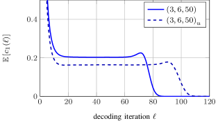
Figure 9: Simulated $\operatorname{\mathbb{E}}\left[c_{1}(\ell)\right]$ for ${(3,6,50)}$ and ${(3,6,50)}_{u}$ at $\epsilon=0.45$.

Since we focus only on the graph evolution for protograph-based codes, Fig. 9 compares simulated results for $\operatorname{\mathbb{E}}\left[c_{1}(\ell)\right]$ at $\epsilon=0.45$ for the ${(3,6,50)}$ and the ${(3,6,50)}_{u}$ ensemble averaged over $5000$ transmissions. We refer to the phase where $c_{1}(\ell)$ is constant as critical phase, and use for it the symbol $c_{1}(*)$. Observe that $c_{1}(*)$ is lower for the ${(3,6,50)}_{u}$ ensemble, similar to what was observed for SPD in [10]. Thus, more iterations are needed to recover all VNs which results also in a longer critical phase. Having a longer critical phase with lower $c_{1}(*)$ also explains why the ${(3,6,50)}_{u}$ ensemble performs worse as observed in [10].

IV Towards Finite-Length Analysis for BP

The smaller $(\epsilon^{*}-\epsilon)$ is, the more iterations are needed for decoding. As in [12], we define the normalized time $\tau$ for the PPD and BP as

$$\tau=\ell\cdot(\epsilon^{*}-\epsilon)$$ (5)

so that the previous iteration is $\tau-(\epsilon^{*}-\epsilon)$.

The initial channel erasure probability of a VN is denoted with $\epsilon$. We extend the notation and denote by $\epsilon(\tau)$ the average erasure probability of VNs in iteration $\tau$. Note that $\epsilon(\tau)$ can be calculated in two ways. On one hand, $\epsilon(\tau)$ can be calculated with the evolution described in Section III-F. On the other hand, we can also apply DE for BP which is discussed in Appendix C. DE for the BEC has low complexity and is a common analysis tool.

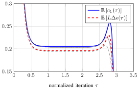
Figure 10: $\operatorname{\mathbb{E}}\left[c_{1}(\tau)\right]$ and $\operatorname{\mathbb{E}}\left[L\Delta\epsilon(\tau)\right]$ for ${(3,6,50)}$. Simulated results are plotted as gray lines for verification.

In general, the complexity of calculating the SPD graph evolution is much higher than for DE. For each CN type $\mathbf{c}\in\mathcal{F}_{c}$, we have $|\overline{\mathcal{F}}_{\mathbf{c}}|=2^{d_{c}}$ types after transmission considered during the graph evolution and only $d_{c}$ erasure probabilities. In total, there are $|\overline{\mathcal{F}}_{c}|$ CN types to track for graph evolution whereas for DE, we only need to track the erasure probabilities of $m=\sum_{\mathbf{c}\in\mathcal{F}}d_{c}$ edge types. As an example, consider again the ${(3,6,3)}$ example from Fig. 2 with $M=4000$ and $\epsilon=0.45$. We have $|\overline{\mathcal{F}}_{c}|=104$ CN types in $\overline{\mathcal{F}}_{c}$ and therefore $104$ CN types need to be tracked during $\ell=4500$ iterations of the graph evolution. Using DE, there are only $18$ erasure probabilities to track for the respective edge types of the code ensemble and we need only $6$ iterations.

Denote with $\Delta\epsilon$ the change of $\epsilon$ between two consecutive iterations. In order to compare $c_{1}(\tau)$ with the decrease of erased VNs, we propose to study a random process based on $\epsilon(\tau)$

$$L\Delta\epsilon(\tau)=L[\epsilon(\tau-(\epsilon^{*}-\epsilon))-\epsilon(\tau)]$$ (6)

which refers to the number of variable nodes resolved per BP iteration of a SC-LDPC code ensemble with $L$ coupled codes, normalized by $M$ as done in (3). This decrease in erasure probability is closely related to the convergence speed [17] where the velocity of the propagation wave is measured. There, in place of the total decrease in erasure probability per iteration, it was analyzed how many iterations $\ell+I,\,I\in\mathbb{N}$, it takes until the erasure probabilities of the VNs at code position $u+1$ are reduced to the erasure probabilities of the VNs at positions $u$ in iteration $\ell$.

Fig. 10 shows the analytical predictions of $\operatorname{\mathbb{E}}\left[c_{1}(\tau)\right]$ and $\operatorname{\mathbb{E}}\left[L\Delta\epsilon(\tau)\right]$ verified with $5000$ transmissions for a ${(3,6,50)}$ code with $M=4000$. Simulation and prediction fit accurately. Observe $\operatorname{\mathbb{E}}\left[c_{1}(\tau)\right]\geq\operatorname{\mathbb{E}}\left[L\Delta\epsilon(\tau)\right]$ in the critical phase. This motivates the use of $\Delta\epsilon(\tau)$ as a surrogate for $c_{1}(\tau)$ and we can state that in fact, $c_{1}(\tau-(\epsilon^{*}-\epsilon))$ is an upper bound of $L\Delta\epsilon(\tau)$.

Theorem IV.1

Assume transmission over a BEC. For any PPD and BP process, $c_{1}(\tau-(\epsilon^{*}-\epsilon))$ is an upper bound on $L\Delta\epsilon(\tau)$:

$$L\Delta\epsilon(\tau)\leq c_{1}(\tau-(\epsilon^{*}-\epsilon)).$$ (7)

Proof.

We normalize with respect to $M$ and $\tau$. $L\Delta\epsilon(\tau)$ VNs are resolved in an iteration. VNs can only be resolved if they are connected to a deg-1 CN and every deg-1 CN can resolve a single VN of the residual graph as discussed in Section III-E. We know that in iteration $\tau$, $c_{1}(\tau-(\epsilon^{*}-\epsilon))$ deg-1 CNs will be resolved. If every of these resolved CNs is connected to a different VN, $c_{1}(\tau-(\epsilon^{*}-\epsilon))$ VNs will be resolved. If $j\geq 1$ deg-1 CNs are connected to any VN $v$, $c_{1}(\tau-(\epsilon^{*}-\epsilon))-\tfrac{(j-1)}{M}$ VNs will be resolved. Thus, it is not possible to resolve more VNs. ∎

IV-A Mean Evolution During the Decoding Process

As mentioned before, DE can be applied in order to compute $\mathbb{E}[\epsilon(\tau)]$ and thus to evaluate the process $\operatorname{\mathbb{E}}\left[L\Delta\epsilon(\tau)\right]$. The DE solution to $\operatorname{\mathbb{E}}\left[L\Delta\epsilon(\tau)\right]$ can be used not only to characterize the asymptotic behavior, i.e. to compute the decoding threshold of the ensemble, but also to determine quantities needed to assess the finite-length performance of the code. Similar to [8], the average error probability over the ensemble of codes is dominated by the probability that the process $\Delta{\epsilon}(\tau)$ survives, i.e. it does not hit the zero plane. Therefore, characterizing the critical phase and $\Delta{\epsilon}(\tau)$ at that time determines the SC-LDPC finite-length performance.

IV-B Analysis of the Moments of $\Delta\epsilon(\tau)$

We approximate the expected fraction of recovered VNs per coupled code during the critical phase, for $\epsilon$ close to $\epsilon^{*}$, with

$$L\Delta\epsilon(\tau)\approx\gamma(\epsilon^{*}-\epsilon),$$ (8)

where $\gamma$ is a positive constant. As shown in Fig. 11, this approximation is reasonable and accurate.

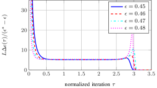
Figure 11: $\operatorname{\mathbb{E}}\left[L\Delta{\epsilon}(\tau)/(\epsilon^{*}-\epsilon)\right]$ for the ${(3,6,50)}$ ensemble.

We approximate $\operatorname{Var}\left[L\Delta{\epsilon}(\tau)\right]$ during the decoding process with $\delta=M\operatorname{Var}\left[L\Delta{\epsilon}(*)\right]$ during the critical phase. Observe in Fig. 12 (a) that $\delta$ is constant for different $(\epsilon^{*}-\epsilon)$.

We also examine $\operatorname{Cov}\left[L\Delta{\epsilon}(\tau),L\Delta{\epsilon}(\tau^{\prime})\right]$ during the decoding process. Fig. 12 (b) shows $\operatorname{Cov}\left[L\Delta\epsilon(\tau),L\Delta\epsilon(\tau^{\prime})\right]$ for $\tau^{\prime}=1.5$ and $\tau^{\prime}=1.75$ during the critical phase of the decoding. Observe that the decay of $\operatorname{Cov}\left[L\Delta{\epsilon}(\tau),L\Delta{\epsilon}(\tau^{\prime})\right]$ behaves similar for both values of $\tau^{\prime}$ during the critical phase.

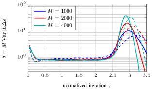
(a)

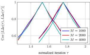
(b)

Figure 12: In (a), simulated and normalized $M\operatorname{Var}\left[L\Delta\epsilon(\tau)\right]$ for the ${(3,6,50)}$ ensemble with $M=\{1000,2000,4000\}$ and $\epsilon=0.45$ (solid), respectively $\epsilon=0.46$ (dashed) from $5000$ simulated transmissions. In (b), simulated $\operatorname{Cov}\left[L\Delta\epsilon(\tau),L\Delta\epsilon(\tau^{\prime})\right]$ for the ${(3,6,50)}$ ensemble with $M=\{1000,2000,4000\}$ and $\epsilon=0.45$ for $\tau^{\prime}=1.5$ and $\tau^{\prime}=1.75$.

IV-C Stability of the Process During the Critical Phase

We now compare the ratios

$$\alpha_{c_{1}}(\tau) =\frac{\operatorname{\mathbb{E}}\left[c_{1}(\tau)\right]}{\sqrt{\operatorname{Var}\left[c_{1}(\tau)\right]}}, \alpha_{\Delta\epsilon}(\tau) =\frac{\operatorname{\mathbb{E}}\left[\Delta\epsilon(\tau)\right]}{\sqrt{\operatorname{Var}\left[\Delta\epsilon(\tau)\right]}}.$$ (9)

Note that $\alpha_{L\Delta\epsilon}(\tau)=\alpha_{\Delta\epsilon}(\tau)$ so that the normalization with $L$ is not needed. The two quantities are plotted for the ${(3,6,50)}$ code with $M=4000$ in Fig. 13. Observe that during the whole decoding process, they are very close. In the critical phase, we have $\alpha_{c_{1}}=6.049$ and $\alpha_{\Delta\epsilon}=6.376$ as listed in Table I.

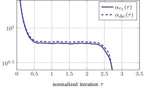
Figure 13: $\alpha_{c_{1}}(\tau)$ and $\alpha_{\Delta\epsilon}(\tau)$ for ${(3,6,50)}$.

V Statistical Models for Failure Probabilities

Given the above results, it is reasonable to follow the argumentation for $c_{1}(\tau)$ and SPD in [8] and to model $\Delta\epsilon$ as a Markov process. For SC-LDPC codes, mean and variance are constant in the critical phase as for $c_{1}$ in [9], and we extend the model of $\Delta\epsilon$ to a Stationary Gaussian Markov process, more specifically to an Ornstein-Uhlenbeck (OU) process. Since the decoding fails when $\Delta\epsilon(\tau)$ hits $0$ before the decoding finishes, we consider the first-passage time (FPT) across $0$ of such a process.

V-A Ornstein-Uhlenbeck Processes

Let $t_{1}<\dots<t_{n}$. A stationary Gaussian Markov Process is also called OU process if $X(t_{1}),\dots,X(t_{n})$ are jointly distributed as a multivariate Gaussian distribution where mean and variance are constant and $\operatorname{Cov}\left[X(t+T),X(t)\right]\propto\exp^{-\alpha T}$ with constant $\alpha>0$, and $T>0$. The OU process is obtained by adding a state-dependent drift to a Wiener process [18]:

$$\mathrm{d}X(t)=-\Theta(\mu-X(t))\mathrm{d}t+\sigma\mathrm{d}W(t),$$ (10)

where $W(\cdot)$ denotes a standard Wiener process and $X(\cdot)$ is the unknown. Let the process start in its mean value so that $\mu=X(0)=x_{0}$. Using $f(X(t),t)=X(t)\operatorname{e}^{\Theta t}$[19], we have

$$\!\!X(t)=x_{0}\operatorname{e}^{-\Theta t}+\mu(1-\operatorname{e}^{-\Theta t})+\operatorname{e}^{-\Theta t}\int_{0}^{t}\sigma\operatorname{e}^{\Theta s}\mathrm{d}W(s),$$ (11)

with $\sigma=\sqrt{2b}$ as in [9]. Since $x_{0}$ is a constant, we have

$$X(t) \sim\mathcal{N}\left(x_{0},\frac{b}{\Theta}\right)$$ (12)

and the expectation of the mean is $\operatorname{\mathbb{E}}\left[X(t)\right]=x_{0}$. Assume that $\min(t,u)=t$. For the covariance, we have

$$\operatorname{Cov}\left[X(t),X(u)\right] \approx\frac{b}{\Theta}\left(\operatorname{e}^{-\Theta|t-u|}\right)$$ (13)

for sufficiently large $t+u$. With the observed quantities from Section IV-B, we have

$$\operatorname{\mathbb{E}}\left[X(t)\right] =x_{0}=\gamma(\epsilon^{*}-\epsilon),$$ (14)

$$\operatorname{Var}\left[X(t)\right] =\frac{b}{\Theta}=\frac{\delta}{M}.$$ (15)

V-B First-Passage Time Distribution

We analyze the average time when $\Delta\epsilon(\tau)$ takes the value $0$ the first time. Using the symmetry of OU processes, we change the initial state to $X(0)=0$ and set a fixed boundary $s=x_{0}$. We define the FPT $T_{s}$ as the time period before the first crossing in $s$:

$$T_{s}=\inf_{t\geq 0}\{t:X(t)\geq s\}.$$ (16)

Denote by $\mu_{0}=\operatorname{\mathbb{E}}\left[T_{s}\right]$ the mean FPT from the zero initial state to the boundary $s$. Evaluating the pdf of $T_{s}$ becomes a complex problem when $\tfrac{s}{b/\Theta}\rightarrow 0$ without any existing closed-form expression [20]. For a reasonably large ratio $\tfrac{s}{b/\Theta}$, it is shown in [21] that the pdf of the FPT converges to an exponential distribution

$$p_{T_{s}}\left(t\right)\sim\frac{1}{\mu_{0}}\operatorname{e}^{\tfrac{-t}{\mu_{0}}},$$ (17)

and according to [21, 22], $\mu_{0}$ can be explicitly calculated with

$$\mu_{0}= \frac{\sqrt{2\pi}}{\Theta}\int_{0}^{\tfrac{s}{\sqrt{b/\Theta}}}\Phi(z)\operatorname{e}^{\tfrac{1}{2}z^{2}}\mathrm{d}z$$

$$= \frac{\sqrt{2\pi}}{\Theta}\int_{0}^{\tfrac{\gamma}{\sqrt{\delta_{1}}}\sqrt{M}(\epsilon^{*}-\epsilon)}\Phi(z)\operatorname{e}^{\tfrac{1}{2}z^{2}}\mathrm{d}z$$ (18)

where $\Phi(z)$ is the cdf of the standard Gaussian distribution.

V-C The Scaling Law for $\Delta\epsilon(\tau)$

The smaller $(\epsilon^{*}-\epsilon)$ is, the more iterations are needed for decoding. For $\epsilon$ very close to $\epsilon^{*}$, it is reasonable to model the decoding process as a continuous-time process as done in [8] for SPD. Similar to [8], the average error probability over the ensemble of codes is dominated by the probability that the process $\Delta{\epsilon}(\tau)$ survives, i.e. it does not hit the zero plane. Therefore, characterizing the critical points and the expected $\Delta{\epsilon}(\tau)$ at that time determines the SC-LDPC finite-length performance.

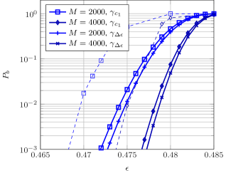
(a)

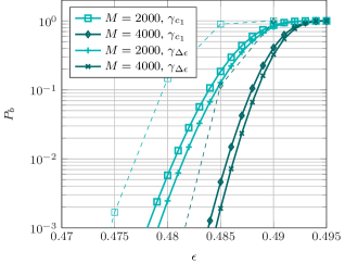
(b)

Figure 14: Predicted trajectories for ${(3,6,100)}$ in (a) and ${(4,8,100)}$ in (b) for $M=\{2000,4000\}$ using $\gamma_{c_{1}}$ and $\gamma_{\Delta\epsilon}$. Simulated results are included as dashed lines.

Based on the statistics describing the $\Delta\epsilon(\cdot)$ process, we model its critical phase with an OU process as described in Section V-B. Denote with $\tau_{\text{eff}}$ the duration of the critical phase of a decoding process:

$$\tau_{\text{eff}} =\tau_{\text{predicted}}-\tau_{\text{corr}}=t_{\text{predicted}}(\epsilon^{*}-\epsilon)-\tau_{\text{corr}},$$ (19)

where $\tau_{\text{predicted}}$ is calculated with DE and $\tau_{\text{corr}}$ is a correction term taking into account the time before and after the critical phase. Note that $\tau_{\text{eff}}$ is a function of $L$ and the given ensemble. The probability of a block error $P_{b}^{*}$ equals the probability of a zero-crossing before $\tau_{\text{eff}}$:

$$P_{b}^{*}=\Pr(T_{s}\leq\tau_{\text{eff}})\approx 1-\exp\left(-\frac{\tau_{\text{eff}}}{\mu_{0}}\right),$$ (20)

since with (17), $T_{s}$ is approximately exponentially distributed.

V-D Comparison to Estimates from SPD

The obtained parameters are summarized in Table I. Fig. 14 compares the estimates using $c_{1}(\tau)$ and $\Delta\epsilon(\tau)$ for the ${(3,6,100)}$ and ${(4,8,100)}$ ensembles. The estimate using $\alpha_{c_{1}}$ is almost identical with the one obtained using SPD in [10]. Note that error probability prediction using the $L\Delta\epsilon(\tau)$ provides slightly overconfident estimates, despite it still correctly captures the slope of the simulated error probability curve.

TABLE I: BEC BP threshold $\epsilon^{*}$, $\alpha_{c_{1}}$, $\alpha_{\Delta\epsilon}$, $\Theta$, $\tau_{\text{eff}}$ and $\tau_{\text{corr}}$ for SC-LDPC code ensembles with $L=100$.

	$\epsilon^{*}$	$\alpha_{c_{1}}$	$\alpha_{\Delta\epsilon}$	$\Theta$	$\tau_{\text{eff}}$	$\tau_{\text{corr}}$
${(3,6,100)}$	$0.4881$	$6.049$	$6.376$	$2.0$	$4.73$	$1.37$
${(4,8,100)}$	$0.4977$	$5.112$	$5.390$	$2.0$	$6.96$	$0.91$

VI Summary and Conclusions

We showed that parallel peeling decoding (PPD) and Belief Propagation (BP) resolve exactly the same variable node (VN) in every iteration. Differences between code ensembles can also be observed with PPD. Instead of analyzing $c_{1}(\tau)$, $\Delta\epsilon(\tau)$ can also be used. This is a significant complexity reduction since it can be derived from the less complex BP analysis. For further research, it will be interesting to obtain further moments of $\Delta\epsilon(\tau)$ analytically. A more profound link between the bounds of Aref et. al for the convergence speed and $\Delta\epsilon$ in this work would also be interesting.

VII Acknowledgement

The authors would like to thank Gerhard Kramer and Michael Lentmaier, for the fruitful discussions.

Appendix A Equivalence of PPD and BP

We first show that without stopping sets, both PPD and BP recover exactly the same erased VNs using messages only passed forwards. We will then show that the message sent back using the PPD does not resolve any additional VNs, and thus the two decoders resolve the identical VNs in every iteration if applied to the same residual graph.

A-A Forward Recovery of VNs

We do not consider $\mu_{{v}\rightarrow{c}}(\ell+1)$ sent back from VN $v$ to CN $c$ as a function of $\mu_{{c}\rightarrow{v}}(\ell)$ so that this analysis holds for both decoders.

Assume a residual graph without any stopping set $\mathcal{S}$. Denote by $\mathcal{C}_{i}(\ell)$ the set of all CNs in the residual graph connected to unknown VNs $i$ times in iteration $\ell$. We divide all CNs in the residual graph into classes:

• $\mathcal{C}_{1}(\ell)$: CNs connected to unknown VNs once in iteration $\ell$,

• $\mathcal{C}_{\geq 2}(\ell)$: CNs connected to unknown VNs two or more times.

Since the CNs in $\mathcal{C}_{1}(\ell)$ are connected to only one unknown VN, both decoders can resolve these VNs in iteration $\ell$. VNs connected only to $\mathcal{C}_{\geq 2}(\ell)$ cannot be resolved by neither of the two decoders. Therefore, these VNs do not change their state and remain erased in iteration $\ell$.

First iteration

Since the residual graph does not contain any stopping set, it must be resolvable with any of these decoders according to [16]. Thus, there must be at least one CN $c$ connected to only one erased VN $v$, i.e. $\mathcal{C}_{1}(\ell)$ is non-empty. An example is depicted in Fig. 15.

All other $\mu_{{v^{\prime}}\rightarrow{c}}(\ell),v^{\prime}\in\mathcal{N}_{c}\setminus\{v\}$ apart from $\mu_{{v}\rightarrow{c}}(\ell)$ are known from the transmission. Since $\mu_{{c}\rightarrow{v}}(\ell)=f(\mu_{{v^{\prime}}\rightarrow{c}}(\ell))$, $v$ cannot get erased again in any later iterations $\ell+i$. If there is another CN $c^{\prime}\in\mathcal{N}_{v}\setminus\{c\}$ , $\mu_{{v}\rightarrow{c^{\prime}}}(\ell+1)$ will be resolved. Since $\mu_{{v}\rightarrow{c^{\prime}}}(\ell)$ is resolved as soon as any other CN $\in\mathcal{N}_{v}$ sends a resolved message to $v$, it will stay resolved independently of the state of the other CNs $\in\mathcal{N}_{v}$ in any later iterations $\ell+i$. If $c^{\prime}$ has degree $j$ in the first iteration and is connected to $k$ resolved VNs, $c^{\prime}\in\mathcal{C}_{j-k}(2)$ of the following iteration.

Figure 15: VN $v$ resolved by CN $v$ forwarding the solution.

$\ell-th$ iteration

If $\mathcal{C}_{1}(\ell)$ is non-empty and contains any CN $c$, the connected unknown VNs are resolved. If there is any CN $c^{\prime}\in\mathcal{C}_{j}(\ell)$, $j>1$, connected to $k$ such resolved VNs, $c^{\prime}$ will be in $\mathcal{C}_{j-k}(\ell+\!1)$. $\mu_{{c^{\prime}}\rightarrow{v}}(\ell+\!1)$ will again stay resolved since they are a function of $c\in\mathcal{C}_{1}(\ell)$ whose messages cannot become erased again.

If $\mathcal{C}_{1}(\ell)$ is empty, the decoding process does not resolve any further VNs and stops. The residual graph does not contain any VNs any more since without any $\mathcal{S}$, it would contain at least a CN connected to only one erased VN.

Graphs with stopping sets

The set $\mathcal{C}_{\geq 2}(\ell)$ is defined as the set that contains all CNs connected to remaining unknown VNs at least twice. This set also includes CNs connected to stopping sets. Denote CNs connected to $\mathcal{S}$ with $\overline{\mathcal{S}}$. Since messages sent from $\overline{}\mathcal{S}$ to the rest of the residual graph can never be resolved during the decoding process, we replace $\overline{}\mathcal{S}$ with erased messages sent from $\overline{}\mathcal{S}$ to the rest of the residual graph as illustrated with an example in Fig. 16.

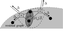
Figure 16: Residual graph including $\overline{}\mathcal{S}$ and $\mathcal{S}$.

The CNs in $\overline{}\mathcal{S}$ are a part of $\mathcal{C}_{\geq 2}(\ell)$ and therefore do not change and stay erased during all iterations. Using any of the two decoders, the decoding of the VNs of the residual graph proceeds identically until $\mathcal{C}_{1}(\ell)$ is empty.

A-B Backward messages of VNs

The decoding of any part of the residual graph depends only on messages sent forward into the residual graph of the respective iteration. Since VNs outside the residual graph are already known, messages sent back outside the residual graph cannot recover any additional VNs.

Theorem A.1

PPD and BP recover exactly the same VNs at each iteration.

Proof.

Using PPD, the message fed back also changes to resolved once a VN is known. The decoding proceeds by resolving the residual graph per iteration which does not depend on the message fed back to the graph outside the residual graph. Thus, PPD and BP recover exactly the same VNs in every iteration. ∎

A-C Observation for messages fed back

Using BP, messages sent back outside the graph are only resolved if a VN is connected to two CNs of $\mathcal{C}_{1}(\ell)$ in any iteration $\ell$.

Appendix B Expected Graph Evolution in a Single Iteration of PPD

Assume we know the graph DD $\{l_{\mathbf{v}}(\ell),r_{\mathbf{c}}(\ell)\}_{\mathbf{v}\in\mathcal{F}_{v},\mathbf{c}\in\overline{\mathcal{F}}_{c}}$ at a particular time $\ell$. We compute the expected graph DD evolution for the next iteration

$$\mathbb{E}[R_{\mathbf{c}}(\ell+1)-R_{\mathbf{c}}(\ell)\Big{|}\{l_{\mathbf{v}}(\ell),r_{\mathbf{c}}(\ell)\}_{\mathbf{v}\in\mathcal{F}_{v},\mathbf{c}\in\overline{\mathcal{F}}_{c}}].$$ (21)

Using the PPD, only deg-1 CNs can be removed directly and in an iteration, we remove all deg-1 CNs along with all VNs connected to them and edges attached to these VNs. Removing these edges resolves also edges for some other CNs and the VNs are connected with as well, so that the type of such a CN is modified from $\mathbf{c}_{1}\in\overline{\mathcal{F}}_{c}$ to $\mathbf{c}_{2}\in\overline{\mathcal{F}}_{c}$. We therefore have an indirect removal of a CN of type $\mathbf{c}_{1}$ from the residual graph and an insertion of a CN of type $\mathbf{c}_{2}$. We assume that by lifting the constructions as described in Section II we obtain independent edges.

The calculation of the graph evolution is outlined as follows:

• For each VN type, calculate the number of edges of an edge type being resolved directly. Take into account that all edges connected to this VN type are in the residual graph and an edge can be resolved by multiple deg-1 CNs.

• For each non-deg-1 CN type in the residual graph, calculate the probability of being connected to any resolved VN and resolving the connecting edges indirectly.

Directly resolved edge types

Any deg-1 CN of type $\mathbf{e}_{j},j\in[1,m]$ is directly removed from the graph as depicted in Fig. 17. To track the changes in the graph, we change to an edge perspective. Denote with $\mathbf{p}_{\text{dir}}(\ell)=(P^{\text{dir}}_{{1}}(\ell),\dots,P^{\text{dir}}_{{m}}(\ell))$ the probability that an edge of a particular type is directly removed from the graph. Assume that messages along different edges are independent due to the lifting with large $N$. $P^{\text{dir}}_{{j}}(\ell)$ can be calculated with

$$P^{\text{dir}}_{{j}}(\ell)=\frac{r_{\mathbf{e}_{j}}(\ell)}{\displaystyle\sum_{\mathbf{c}:c_{j}>0}r_{\mathbf{c}}(\ell)},$$ (22)

for $j=1,\ldots,m$, which we define to be $0$ for $r_{\mathbf{e}_{j}}(\ell)=0$.

Resolved VN types

A VN of type $\mathbf{v}$ is resolved if it is connected to at least one deg-1 CN. Having $l_{\mathbf{v}}(\ell)$ VNs of a specific type, we obtain the number of resolved VNs of type $\mathbf{v}$ with

$$l_{\mathbf{v}}(\ell)\left(1-(\mathbf{1}-\mathbf{p}_{\text{dir}}(\ell))^{\mathbf{v}}\right).$$ (23)

Note that we assume that the probability that an edge type is directly removed is independent of the removal of other edges in the graph.

Indirectly resolved edge types

Denote with $P_{j,\text{indir}}(\ell)$ the probability that an edge of type $j$ was resolved indirectly. These edges of type $j$ are not connected to a deg-1 CN but to any other possible CN of type $\mathbf{c}$ in the residual graph with $c_{j}>0$:

$$P_{j,\text{indir}}(\ell) =(1-P^{\text{dir}}_{{j}}(\ell))\cdot\left(1-(\mathbf{1}-\mathbf{p}_{\text{dir}}(\ell))^{\mathbf{v}-\mathbf{e}_{j}}\right).$$ (24)

The total number of indirectly resolved edges of type $j$ in the residual graph is obtained with

$$\sum_{\mathbf{c}:c_{j}>0}r_{\mathbf{c}}P_{j,\text{indir}}(\ell).$$ (25)

Indirectly resolved edges of CN types

Denote with $\mathbf{p}_{\mathbf{c},\text{indir}}(\ell)=(P_{\mathbf{c},1,\text{indir}}(\ell),\dots,P_{\mathbf{c},m,\text{indir}}(\ell))$ the probabilities that a CN of type $\mathbf{c}$, $|\mathbf{c}|>1$, is connected to a resolved VN via a specific edge type $j=1,\dots,m$. Using (22) and (24), we calculate $P_{\mathbf{c},j,\text{indir}}(\ell)$ with

$$P_{\mathbf{c},j,\text{indir}}(\ell) =\frac{r_{\mathbf{c}}}{\displaystyle\sum_{\begin{subarray}{c}\mathbf{c}^{\prime}:c_{j}>0\\ |\mathbf{c}^{\prime}|>1\end{subarray}}r_{\mathbf{c}^{\prime}}}\cdot P_{j,\text{indir}}(\ell)$$

$$=\frac{r_{\mathbf{c}}}{\displaystyle\sum_{\begin{subarray}{c}\mathbf{c}^{\prime}:c_{j}>0\\ |\mathbf{c}^{\prime}|>1\end{subarray}}r_{\mathbf{c}^{\prime}}}\cdot\frac{\sum_{\mathbf{c}:c_{j}>0}r_{\mathbf{c}}(\ell)-r_{\mathbf{e}_{j}}(\ell)}{\displaystyle\sum_{\mathbf{c}:c_{j}>0}r_{\mathbf{c}}(\ell)}$$

$$\cdot\left(1-(\mathbf{1}-\mathbf{p}_{\text{dir}}(\ell))^{\mathbf{v}-\mathbf{e}_{j}}\right)$$

$$=\frac{r_{\mathbf{c}}}{\displaystyle\sum_{\mathbf{c}^{\prime}:c_{j}>0}r_{\mathbf{c}^{\prime}}}\cdot\left(1-(\mathbf{1}-\mathbf{p}_{\text{dir}}(\ell))^{\mathbf{v}-\mathbf{e}_{j}}\right).$$ (26)

An indirect resolving of an edge connected to a CN of type $\mathbf{c}$ is illustrated in Fig. 17. We can now calculate the number of indirectly resolved CNs of type $\mathbf{c}$ which we denote with $E^{-}_{\mathbf{c}}(\ell)$:

$$E^{-}_{\mathbf{c}}(\ell) =r_{\mathbf{c}}(\ell)(\mathbf{p}_{\mathbf{c},\text{indir}}(\ell))^{\mathbf{c}}.$$ (27)

Figure 17: VN $\mathbf{v}$ connected to a CN of type $e_{j}$ resolving an edge of type $j$, in turn resolving a socket of a CN of type $c$.

Since it is also possible that not all edges of a CN are indirectly resolved, we obtain the fraction of CNs of type $\mathbf{c}$ reduced to a CN of type $\mathbf{c}^{\prime}$ with

$$E^{-}_{\mathbf{c},\mathbf{c}^{\prime}}(\ell)= r_{\mathbf{c}}(\ell)(\mathbf{p}_{\mathbf{c},\text{indir}}(\ell))^{\mathbf{c}-\mathbf{c}^{\prime}}(\mathbf{1}-\mathbf{p}_{\mathbf{c},\text{indir}}(\ell))^{\mathbf{c}^{\prime}}.$$ (28)

This corresponds to resolving all other edges of $\mathbf{c}$ than there are remaining in $\mathbf{c}^{\prime}$.

Indirectly added CN types

CNs of other types can be added to the residual graph if not all edges of an indirectly resolved CN are resolved. From (28), we have

$$E_{\mathbf{c}^{\prime}}^{+}(\ell)=\sum_{\mathbf{c}\in\overline{\mathcal{F}}_{c}}E^{-}_{\mathbf{c},\mathbf{c}^{\prime}}(\ell).$$ (29)

Expected evolution in a single PPD iteration

We now calculate the expected evolution of the number of CNs of type $\mathbf{c}$ in the graph in a single PPD iteration. For any CN type $\mathbf{c}\in\overline{\mathcal{F}}_{c}$ such that $\mathbf{c}\neq\mathbf{e}_{j},j\in[1,m]$, the overall evolution is

$$\mathbb{E}[R_{\mathbf{c}}(\ell+1)-R_{\mathbf{c}}(\ell)]=E_{\mathbf{c}}^{+}(\ell)-E^{-}_{\mathbf{c}}(\ell).$$ (30)

For any deg-1 CN of type $\mathbf{e}_{j},j\in[1,m]$, we have

$$\mathbb{E}[R_{\mathbf{e}_{j}}(\ell+1)-R_{\mathbf{e}_{j}}(\ell)]=E_{\mathbf{e}_{j}}^{+}(\ell)-r_{\mathbf{e}_{j}}(\ell).$$ (31)

Appendix C Density Evolution for BP

We transmit over a BEC. We represent each symbol transmitted with a VN which is erased with probability $\epsilon$. Since PPD and BP are equivalent, $\Delta\epsilon$ can also be obtained from the analysis of BP, for which we apply DE [14]. Denote the erasure probability of the channel with $\epsilon_{ch}$. The erasure probability is tracked for each edge type of the protograph separately. For any edge type $s\in\{1,\dots,m\}$, we denote the erasure probability of messages sent from the VN in iteration $\ell$ with $x_{s}(\ell)$ and from the CN with $y_{s}(\ell)$. We denote them as vectors with

$$\mathbf{x}(\ell) =(x_{1}(\ell),\dots,x_{m}(\ell)),$$ (32)

$$\mathbf{y}(\ell) =(y_{1}(\ell),\dots,y_{m}(\ell)).$$ (33)

Since we calculate edge type erasure probabilities, we do not consider the additional CN types after transmission in the residual graph and we consider the initial CN types $\mathbf{c}\in\mathcal{F}_{c}$. Using the constructions described in Section II, the edge type $s$ is only connected to one VN type $\mathbf{v}\in\mathcal{F}_{v}$ and one CN type $\mathbf{c}\in\mathcal{F}_{c}$. The CN and VN functions can be calculated exactly with

$$y_{s}(\ell) =1-(\mathbf{1}-\mathbf{x}(\ell-1))^{\mathbf{c}-\mathbf{0}_{\sim s}}, \mathbf{c}\in\mathcal{F}_{c},$$ (34)

$$x_{s}(\ell) =\epsilon\mathbf{y}(\ell)^{\mathbf{v}-\mathbf{0}_{\sim s}}, \mathbf{v}\in\mathcal{F}_{v},$$ (35)

where all exponents are $\geq 0$ and punctured VNs types are initialized with $\epsilon=0$. Denote the erasure probability of a VN type $\mathbf{v}\in\mathcal{F}_{v}$ after the $\ell$-th iteration

$$\epsilon_{\mathbf{v}}(\ell) =\epsilon_{ch}\mathbf{y}(\ell)^{\mathbf{v}}, \mathbf{v}\in\mathcal{F}_{v}.$$ (36)

We calculate the erased VNs per iteration with

$$\epsilon(\ell)=\sum_{\mathbf{v}\in\mathcal{F}_{v}}l_{\mathbf{v}}\epsilon_{\mathbf{v}}(\ell).$$ (37)

As shown in [14], $\epsilon_{\mathbf{v}}$ for every VN type $\mathbf{v}\in\mathcal{F}_{v}$ is monotonically decreasing during the decoding process.

References

- [1] S. Kudekar, T. Richardson, and R. Urbanke, “Spatially coupled ensembles universally achieve capacity under belief propagation,” IEEE Trans. Inf. Theory, vol. 59, no. 12, pp. 7761–7813, 2013.
- [2] S. Kumar, A. J. Young, N. Macris, and H. D. Pfister, “Threshold saturation for spatially coupled LDPC and LDGM codes on BMS channels,” IEEE Trans. Inf. Theory, vol. 60, no. 12, pp. 7389–7415, Dec. 2014.
- [3] M. Lentmaier, A. Sridharan, D. J. Costello, and K. S. Zigangirov, “Iterative decoding threshold analysis for LDPC convolutional codes,” IEEE Trans. Inf. Theory, vol. 56, no. 10, pp. 5274–5289, 2010.
- [4] D. G. M. Mitchell, A. E. Pusane, M. Lentmaier, and D. J. Costello, “Exact free distance and trapping set growth rates for LDPC convolutional codes,” in IEEE Int. Symp. Inf. Theory (ISIT), 2011, pp. 1096–1100.
- [5] D. G. M. Mitchell, M. Lentmaier, and D. J. Costello, “Spatially coupled LDPC codes constructed from protographs,” July 2014.
- [6] K. Kasai and K. Sakaniwa, “Spatially-coupled MacKay-Neal codes and Hsu-Anastasopoulos codes,” in Proc. IEEE Int. Symp. Inf. Theory, St. Petersburg, Russia, 2011.
- [7] M. G. Luby, M. Mitzenmacher, M. A. Shokrollahi, and D. A. Spielman, “Efficient erasure correcting codes,” IEEE Trans. Inf. Theory, vol. 47, no. 2, pp. 569–584, 2001.
- [8] A. Amraoui, A. Montanari, T. J. Richardson, and R. L. Urbanke, “Finite-length scaling for iteratively decoded LDPC ensembles,” IEEE Trans. Inf. Theory, vol. 55, no. 2, pp. 473–498, Feb. 2009.
- [9] P. Olmos and R. Urbanke, “A scaling law to predict the finite-length performance of spatially-coupled LDPC codes,” IEEE Trans. Inf. Theory, vol. 61, no. 6, pp. 3164–3184, 2015.
- [10] M. Stinner and P. M. Olmos, “On the waterfall performance of finite-length SC-LDPC codes constructed from protographs,” IEEE J. Sel. Areas Commun., vol. PP, no. 99, p. 1, 2015.
- [11] J. Ezri, A. Montanari, and R. Urbanke, “A generalization of the finite-length scaling approach beyond the BEC,” IEEE Int. Symp. Inf. Theory (ISIT), pp. 1011–1015, June 2007.
- [12] J. Ezri, A. Montanari, S. Oh, and R. L. Urbanke, “The slope scaling parameter for general channels, decoders, and ensembles,” in IEEE Int. Symp. Inf. Theory (ISIT), July 2008, pp. 1443–1447.
- [13] J. Thorpe, “Low-density parity-check (LDPC) codes constructed from protographs,” JPL IPN, Tech. Rep., 2003.
- [14] T. J. Richardson and R. L. Urbanke, Modern Coding Theory. Cambridge University Press, 2008.
- [15] F. R. Kschischang, B. J. Frey, and H.-A. A. Loeliger, “Factor graphs and the sum-product algorithm,” IEEE Trans. Inf. Theory, vol. 47, no. 2, pp. 498–519, 2001.
- [16] C. Di, D. Proietti, I. E. Telatar, T. J. Richardson, and R. L. Urbanke, “Finite-length analysis of low-density parity-check codes on the binary erasure channel,” IEEE Trans. Inf. Theory, vol. 48, no. 6, pp. 1570–1579, June 2002.
- [17] V. Aref, L. Schmalen, and S. Ten Brink, “On the convergence speed of spatially coupled LDPC ensembles,” Allerton Conf. Commun. Control, Computing, 2013, pp. 342–349, 2013.
- [18] C. Gardiner, Stochastic Methods: A Handbook for the Natural and Social Sciences. Springer, 2009.
- [19] I. Karatzas and S. E. Shreve, Brownian Motion and Stochastic Calculus, 2nd ed. Springer, Aug. 1991.
- [20] D. T. Gillespie, “Exact numerical simulation of the Ornstein-Uhlenbeck process and its integral,” Phys. Rev. E. Stat. Phys. Plasmas. Fluids. Relat. Interdiscip. Topics, vol. 54, no. 2, pp. 2084–2091, 1996.
- [21] A. G. Nobile, L. M. Ricciardi, and L. Sacerdote, “Exponential trends of Ornstein-Uhlenbeck first-passage-time densities,” J. Appl. Probab., vol. 22, no. 2, pp. 360–369, 1985.
- [22] M. U. Thomas, “Some mean first-passage time approximations for the Ornstein-Uhlenbeck process,” J. Appl. Probab., vol. 12, no. 3, pp. 600–604, 1975.