Transport in a stochastic Goupillaud medium

Abstract This paper is part of a project that aims at modelling wave propagation in random media by means of Fourier integral operators. A partial aspect is addressed here, namely explicit models of stochastic, highly irregular transport speeds in one-dimensional transport, which will form the basis for more complex models. Starting from the concept of a Goupillaud medium (a layered medium in which the layer thickness is proportional to the propagation speed), a class of stochastic assumptions and limiting procedures leads to characteristic curves that are Lévy processes. Solutions corresponding to discretely layered media are shown to converge to limits as the time step goes to zero (almost surely pointwise almost everywhere). This translates into limits in the Fourier integral operator representations.

1 Introduction

This contribution is part of a long-term project that aims at modelling wave propagation in random media by means of Fourier integral operators. The intended scope includes, for example, the equilibrium equations in linear elasticity theory

$$\rho\frac{\partial^{2}u_{i}}{\partial t^{2}}-\sum_{j,k,l}\frac{\partial}{\partial x_{j}}c_{ijkl}\frac{\partial u_{l}}{\partial x_{k}}=f_{i},\quad i=1,2,3$$

or, more generally, hyperbolic systems of the form

$$\frac{\partial u}{\partial t}=\sum_{j=1}^{m}A_{j}(t,x)\frac{\partial u}{\partial x_{j}}+B(t,x)u+f(t,x),$$ (1)

to be solved for the unknown functions $u(t,x)=(u_{1}(t,x),\cdots,u_{n}(t,x))$. Here $t$ denotes time, $x$ is an $m$-dimensional space variable, and $A_{j}$, $B$ are $(n\times n)$-matrices.

Our specific interest is in the situation where the coefficient matrices are random functions of the space variable $x$, i.e., random fields. Such a situation typically arises in seismology (propagation of acoustic waves) or in material science (damage detection). There are many ways of setting up models for random fields (see e. g. [9, 14]), but typically random fields describing randomly perturbed media have continuous, but not differentiable paths. As coefficients in hyperbolic equations such as (1), this degree of regularity is too low and does not allow one to apply the classical solution theory for hyperbolic equations. In addition, the solution depends nonlinearly on the coefficients, so it is generally impossible to directly calculate the stochastic properties of the solution from knowledge of the distribution of the coefficients.

The main thrust of the project will be to write the solution to equations like (1) as a sum of Fourier integral operators

$$u(t,x)=\frac{1}{(2\pi)^{m}}\iint{\rm e}\hskip 1.0pt^{i\varphi(t,x,y,\eta)}a(t,x,y,\eta)u_{0}(y)\,\hskip 1.0pt{\rm d}\hskip 0.5pty\hskip 1.0pt{\rm d}\hskip 0.5pt\eta$$ (2)

applied to the initial data $u_{0}$. This is possible in the case of deterministic, smooth coefficients (up to a smooth error). The ultimate goal of the project will be to set up the stochastic model of the medium through the phase function $\varphi$ and the amplitude $a$ of the Fourier integral operator, rather than through a direct stochastic model of the coefficients, as described in [16].

A second thrust is in understanding wave propagation in strongly irregular stochastic media with a sufficiently simple structure and tractable properties, in order to get insight into what stochastic processes are suitable to be entered as phase functions and amplitudes. This brings us to the topic of this paper, namely, wave propagation in a Goupillaud medium (the name goes back to [10]). In this contribution, we will work out the case of one-dimensional transport under assumptions that will lead to characteristic curves given by an increasing Lévy process with possibly infinitely many jumps on each subinterval.

One-dimensional transport is described by the equation

$$\begin{array}[]{rcl}\dfrac{\partial}{\partial t}u(t,x)+c(x)\dfrac{\partial}{\partial x}u(t,x)&=&0\\[10.0pt] u(0,x)&=&u_{0}(x)\end{array}$$ (3)

The material properties of the medium are encoded in the transport speed $c(x)$. The Goupillaud assumption is that $c(x)$ is a piecewise constant function so that the travel time in each layer is the same. That is, the thickness of layer number $k$ is proportional to the propagation speed $c_{k}$ in that layer.

Further, the propagation speeds $c_{k}$ will be given by independent, identically distributed random variables. At this stage, various choices of the type of random variables as well as scalings are possible. For the wave equation, such scalings leading to fairly regular limiting processes have been introduced in [5] and studied in [8, 15]. Our procedure of dyadic refinements on the time axis will lead to infinitely divisible, positive random variables. It turns out that they can be constructed as increments of a strictly increasing Lévy process, a so-called subordinator with positive drift. As the time step goes to zero, the characteristic curve of (3) passing through the origin is a path of a Lévy process. We will show that the characteristic curves of the discrete Goupillaud medium converge (almost surely at almost every $(x,t)$) to limiting curves (actually translates of the obtained Lévy process), and that the corresponding solutions and their Fourier integral operator representations converge as well.

The limiting function $u(x,t)$ is constant along the limiting characteristic curves, as in the case of classical transport. However, the limiting characteristics may possibly have infinitely many jumps on each interval. Due to this high degree of singularity, we cannot give a meaning to the limiting function $u(x,t)$ as a solution to (3) – it is just a limit of piecewise classical solutions. This situation is quite common in the theory of singular stochastic partial differential equations, see e.g. [11].

A few remarks about the regularity of the coefficient $c(x)$ in (3) is in order. If the coefficient is Lipschitz continuous, classical solutions can be readily constructed. If the coefficient is a piecewise constant, positive function, piecewise classical solutions are obtained easily. In case of lower regularity of the coefficient, various approaches have been proposed in the literature. We mention the work of DiPerna and Lions [6], Bouchut and James [4], and Ambrosio et al. [1, 2] in the deterministic, $x$-dependent case; for a recent survey, see Haller and Hörmann [12]. In the stochastic case, recent work of Flandoli [7] shows how solutions can be constructed adding noise in the transport term. Finally, another different line of development is constituted by extending the reservoir of generalized functions, either in the direction of white noise analysis or in the direction of Colombeau theory. A representative article pursuing and comparing both approaches is by Pilipović and Seleši [17, 18].

The plan of the paper is as follows: In the first part, the stochastic Goupillaud medium is set up and analyzed. In the second part, the limiting behavior as the time step goes to zero is established. The paper ends with some conclusions and open questions.

2 Setting up the Goupillaud medium

If the initial data $u_{0}$ are differentiable and the propagation speed $c$ is Lipschitz continuous, classical solutions to the transport equation (3) can be readily obtained by the method of characteristics. The characteristic curves are the integral curves of the vector field $\partial/\partial t+c(x)\partial/\partial x$ passing through the point $x$ at time $t$, that is, the solutions to the ordinary differential equation

$$\frac{\,\mathrm{d}}{\,\mathrm{d}\tau}{\gamma}(\tau;x,t)=c(\gamma(\tau;x,t)),\quad\gamma(t;x,t)=x.$$

Then the solution to (3) is given by

$$u(x,t)=u_{0}(\gamma(0;x,t)).$$

Under the mentioned assumptions, the function $u$ is continuously differentiable, and the solution is unique in this class.

If the speed parameter $c$ is constant the characteristic curves are simply given by $\gamma(\tau;x,t)=x+c(\tau-t)$. If the parameter is piecewise constant one can compute the characteristic curves as polygons. Assuming continuity across interfaces, the solution $u$ is given as a continuous, piecewise differentiable function, which solves (3) in the weak sense.

2.1 Dyadic deterministic structure

We begin by setting up the discrete, deterministic Goupillaud medium. Take an equidistant sequence $(t_{j})_{j\in\mathbb{N}}$ of points of time with $t_{0}=0$ and time step $\Delta t\equiv t_{j}-t_{j-1}$ for all $j=1,2,\ldots$. Furthermore, take a strictly increasing sequence $(x_{k})_{k\in\mathbb{Z}}$ with $x_{0}=0$ and $x_{k}\to\pm\infty$ as $k\to\pm\infty$ and let $\Delta x_{k}=x_{k}-x_{k-1}$. The coefficient $c(x)$ is defined as

$$c(x)=\sum_{k=-\infty}^{\infty}\frac{\Delta x_{k}}{\Delta t}\mathds{1}_{[x_{k-1},x_{k})}(x).$$ (4)

In other words, the time for passing a layer $\Delta x_{k}$ is constant, namely $\Delta t$. For an illustration see Figure 1.

Figure 1: Illustration of $\tau\rightarrow\gamma(\tau;0,0)$ in the Goupillaud medium (left). Refining the grid on the right preserves existing grid points $\gamma^{(1)}(\cdot;0,0)$ (dashed) and refinement $\gamma^{(2)}(\cdot;0,0)$.

Call $c_{k}$ the value of $c(x)$ in the $k$-th layer, that is, $x_{k-1}\leq x<x_{k}$. Then the Goupillaud relation

$${\Delta x_{k}}=c_{k}\Delta t$$ (5)

holds for all $k$, with constant $\Delta t$. The structure of the Goupillaud medium makes computing the values of the characteristic curves $\gamma(\tau;x,t)$ in the grid points very simple. In fact,

$$\gamma\left(t_{j};x_{k},t_{l}\right)=x_{j+k-l}$$ (6)

for all integers $j,k,l$. Since every point $(x,t)$ is just a convex combination of the neighboring grid points, the values $\gamma(\tau;x,t)$ can be easily obtained anywhere.

We now set up a dyadic refinement of the initial grid. Define

$$\Delta t^{(N)}=2^{-N},\quad t^{(N)}_{j}=\frac{j}{2^{N}}$$

and let $x^{(N)}_{k}\in\mathbb{R}$, $k\in\mathbb{Z}$, be a strictly increasing sequence of spatial points (or equivalently, propagation speeds $c^{(N)}_{k}>0$ satisfying $\Delta x^{(N)}_{k}=c^{(N)}_{k}\Delta t^{(N)}$). We require that each resulting grid is a dyadic refinement of the previous one, that is

$$\big{(}t^{(N+1)}_{2j},\,x_{2k}^{(N+1)}\big{)}=\big{(}t^{(N)}_{j},\,x_{k}^{(N)}\big{)},$$ (7)

as illustrated in Figure 1. This condition implies

$$\Delta x^{(N)}_{k}=\Delta x^{(N+1)}_{2k-1}+\Delta x^{(N+1)}_{2k}.$$

Inductively, one obtains

$$\quad\Delta x_{k}^{(N)}=\sum_{i=1}^{2^{M}}\Delta x_{(k-1)2^{M}+i}^{(N+M)}$$ (8)

for all $N,M\in\mathbb{N},k\in\mathbb{Z}$. The value of the characteristic curve $\gamma^{(N)}$ in the grid points is readily obtained according to (6). For any integer $N,j,k,l$ we have

$$\gamma^{(N)}\left(t_{j}^{(N)};x_{k}^{(N)},t^{(N)}_{l}\right)=x^{(N)}_{j+k-l}.$$ (9)

For any $N\in\mathbb{N}$ and $\tau\in[t_{k-1}^{(N)},t_{k}^{(N)})$, the characteristic curve through the origin $\xi^{(N)}(\tau)=\gamma^{(N)}(\tau;0,0)$ can be represented as

$$\xi^{(N)}(\tau)=\alpha^{(N)}(\tau)\xi^{(N)}(t_{k-1}^{(N)})+\big{(}1-\alpha^{(N)}(\tau)\big{)}\xi^{(N)}(t_{k}^{(N)}),$$ (10)

where

$$\alpha^{(N)}(\tau)=\frac{t_{k}^{(N)}-\tau}{t_{k}^{(N)}-t_{k-1}^{(N)}}=\big{(}t_{k}^{(N)}-\tau\big{)}2^{N}\in[0,1].$$

and $\xi^{(N)}(t^{(N)}_{k})=x^{(N)}_{k}$ by (9).

In other words, $\xi^{(N)}$ is an increasing polygon through $(t_{k}^{(N)},x_{k}^{(N)})$, $k\in\mathbb{Z}$. For $(x,t)\in\mathbb{R}^{2}$ one obtains the characteristic curve through $(x,t)$ by

$$\gamma^{(N)}(\tau;x,t)=\xi^{(N)}\big{(}\tau+(\xi^{(N)})^{-1}(x)-t\big{)},\quad\tau\in\mathbb{R},$$ (11)

i.e., by shifting $\xi^{(N)}$ in time direction such that it passes through $(x,t)$.

2.2 The stochastic model

In this subsection, we formulate the stochastic assumptions underlying our model of a randomly layered medium, in which $\Delta x_{k}^{(N)}$ is random. In the sequel, we will denote random elements by capital letters and realizations by the corresponding small ones. Let $(\Omega,\mathcal{F},\mathbb{P})$ be a probability space which is rich enough. Our decisive assumption is that for each $N\in\mathbb{N}$, the increments are positive i.i.d. random variables $\Delta X_{k}^{(N)}$, $k\in\mathbb{Z}$,

Together with our previous consistency assumption (8), this implies that $\Delta X_{k}^{(N)}$ is infinitely divisible for every $k\in\mathbb{Z}$ and $N\in\mathbb{N}$ (using e.g. [13, Thm. 15.12]). Let $\mu=\mathbb{P}\circ(\Delta X^{(0)}_{1})^{-1}$ be the distribution of $\Delta X^{(0)}_{1}$. Then $\Delta X_{k}^{(N)}\sim\mu^{*1/2^{N}}$, $k\in\mathbb{N}$, the $2^{N}$-th unique root of $\mu$, cf. [19, p. 34]. Again by [13, Thm. 15.12], there exists a Lévy process $X=(X(t))_{t\in\mathbb{R}}$ on a probability space, w.l.o.g. say $(\Omega,\mathcal{F},\mathbb{P})$, with $\mathbb{P}\circ X(1)^{-1}=\mu$, that is, $\Delta X^{(0)}_{1}$ has the same distribution as $X(1)$. These conditions are met, e.g., by Poisson processes or Gamma processes with positive drift.

Having derived the Lévy process, we may use it as a starting point for defining the stochastic Goupillaud medium. We let $t_{k}^{(N)}=k/2^{N}$ as in subsection 2.1 and define

$$\Delta X_{k}^{(N)}=X\big{(}t_{k}^{(N)}\big{)}-X\big{(}t_{k-1}^{(N)}\big{)}$$

and

$$X_{k}^{(N)}=\sum_{i=1}^{k}\Delta X_{i}^{(N)}=X\big{(}t_{k}^{(N)}\big{)}$$

for $k>0$ and similarly for $k\leq 0$. The consistency condition (8) is clearly satisfied. Let furthermore $X^{(N)}(\omega,\cdot)$ be the piecewise affine interpolation of $X(\omega,\cdot)$ through the grid points $(t_{k}^{(N)},X_{k}^{(N)})$ as in (10). This construction is carried out pathwise for fixed $\omega\in\Omega$.

3 Limits as the time step goes to zero

The main result of this section is that the characteristic curves of the discrete Goupillaud medium converge to limiting curves (almost surely almost everywhere). This will imply that the solutions to the transport equation converge to a limit as well (in a sense to be made precise). The crucial observation is that the paths of a Lévy process are càdlàg almost surely, i.e., they are continuous from the right and have left-hand limits.

3.1 A convergence result for càdlàg functions

The first convergence result holds generally for càdlàg functions. Thus let $t\to\xi(t)$ be an increasing càdlàg function with $\xi(t)\rightarrow\pm\infty$ for $t\rightarrow\pm\infty$ and let $(x,t)\in\mathbb{R}^{2}$. Set

$$\xi^{*}(x)=\inf\left\{t\in\mathbb{R}:\xi(t)\geq x\right\}$$

which is Borel measurable, and

$$\gamma(\tau;x,t)=\xi(\tau+\xi^{*}(x)-t),\quad\tau\in\mathbb{R}.$$

Further, let $\xi^{(N)}$ be a piecewise linear interpolation of $\xi$ that coincides with $\xi$ at the grid points $t_{k}^{(N)}=k/2^{N}$, $k\geq 0$, and define $\gamma^{(N)}(\tau;x,t)$ by formula (11).

Lemma 3.1.

Let $(x,t)\in\mathbb{R}^{2}$, $\xi$, $\xi^{(N)}$, $\gamma$, $\gamma^{(N)}$ as described above. If the function $\tau\to\gamma(\tau;x,t)$ does not have a jump in $\tau_{0}$, then

$$\lim_{N\to\infty}\gamma^{(N)}(\tau_{0};x,t)=\gamma(\tau_{0};x,t),$$

i.e., $\gamma^{(N)}(\,\cdot\,;x,t)$ converges pointwise to $\gamma(\,\cdot\,;x,t)$ at the points of continuity of $\gamma(\,\cdot\,;x,t)$.

Proof.

Fix $\varepsilon>0$ and $R>|\tau_{0}|+|\xi^{*}(x)|+|t|$ and define

$$s :=\tau_{0}+\xi^{*}(x)-t$$

$$s^{(N)} :=\tau_{0}+(\xi^{(N)})^{-1}(x)-t$$

As $\xi$ is càdlàg there exist finitely many $(t_{1},\ldots,t_{\ell})\in[-R,R]$ such that

$$\forall r_{1},r_{2}\in[t_{i},t_{i+1}):\left|\xi(r_{1})-\xi(r_{2})\right|<\frac{\varepsilon}{3},$$ (12)

see e.g. [3, Lemma 1, p. 110]. Since $\gamma$ is continuous in $\tau_{0}$ we can assume without loss of generality that $s\neq t_{i}$ for all $i$.

Since $\xi$ and $\xi^{(N)}$ coincide at the grid points and both are increasing, $(\xi^{(N)})^{-1}(x)$ and $\xi^{*}(x)$ belong to the same interval of length $1/2^{N}$, for every $N$. It follows that $|s^{(N)}-s|<1/2^{N}$ as well. We can choose $N$ large enough, such that both $s$ and $s^{(N)}$ belong to $(t_{i}+1/2^{N},t_{i+1}-1/2^{N})$ for some $i\in\{1,\ldots,\ell-1\}$. From (12) we get that

$$\left|\gamma^{(N)}(\tau_{0};x,t)-\gamma(\tau_{0};x,t)\right|=\left|\xi^{(N)}(s^{(N)})-\xi(s)\right|\leq\left|\xi^{(N)}(s^{(N)})-\xi(s^{(N)})\right|+\frac{\varepsilon}{3}.$$

Now choose $k$ such that

$$t_{i}<t_{k-1}^{(N)}\leq s^{(N)}\leq t_{k}^{(N)}<t_{i+1}.$$

Using (10) and the fact that $\xi$ and $\xi^{(N)}$ coincide at all grid points $t_{j}^{(N)}$ we can write

$$\xi^{(N)}(s^{(N)})-\xi(s^{(N)}) = \alpha^{(N)}(s^{(N)})\xi(t_{k-1}^{(N)})+\big{(}1-\alpha^{(N)}(s^{(N)})\big{)}\xi(t_{k}^{(N)})-\xi(s^{(N)})$$

$$= \big{(}1-\alpha^{(N)}(s^{(N)})\big{)}\big{(}\xi(t_{k}^{(N)})-\xi(t_{k-1}^{(N)})\big{)}+\big{(}\xi(t_{k-1}^{(N)})-\xi(s^{(N)}\big{)}.$$

Recalling $\alpha^{(N)}\in[0,1]$ for all $N$ and invoking again (12) we conclude that

$$\left|\gamma^{(N)}(\tau_{0};x,t)-\gamma(\tau_{0};x,t)\right|<\varepsilon,$$

which implies the desired convergence. ∎∎

Denote by $T=(T_{i})_{i\in\mathbb{N}}$ the (countable) set of jump points of the càdlàg function $\xi$. At fixed $(x,t)$, convergence may fail at those values $\tau$ for which $\tau+\xi^{*}(x)-t\in T$. This exceptional set is countable, but may be different for every $(x,t)$. Next, we fix $\tau_{0}$ and determine the set of all $(x,t)$ for which convergence fails. We are going to show that its two-dimensional Lebesgue measure $\lambda$ is zero.

Lemma 3.2.

Let $\tau_{0}\geq 0$; $\xi$, $\gamma$ as in Lemma 3.1. The set $M=\{(x,t):\gamma(\tau;x,t)\ {\rm jumps}\ {\rm at}\ \tau_{0}\}$ has Lebesgue measure zero.

Proof.

Letting

$$M=\{(x,t):\tau_{0}+\xi^{*}(x)-t\in T\}=\bigcup_{i\in\mathbb{N}}M_{i}$$

where $M_{i}=\{(x,t):\tau_{0}+\xi^{*}(x)-t=T_{i}\}$, it suffices to check that each $M_{i}$ has Lebesgue measure zero. But each $M_{i}$ is jointly measurable, and for each $x$ the set $M_{i}(x)=\{t:\tau_{0}+\xi^{*}(x)-t=T_{i}\}$ is a singleton. Hence

$$\lambda(M_{i})=\int_{\mathbb{R}}\lambda(M_{i}(x))\,\mathrm{d}x=0$$

by Fubini’s theorem. ∎∎

3.2 Convergence of characteristic curves

We now apply Lemma 3.1 to a path $t\to X(\omega,t)=\xi(t)$ of the Lévy process $X$ constructed in subsection 2.2. Since Lévy processes are càdlàg almost surely, there is $\Omega_{0}\in\mathcal{F}$ with $\mathbb{P}(\Omega_{0})=1$ such that $X(\omega,\cdot)$ is càdlàg for all $\omega\in\Omega_{0}$. With the notation of subsections 2.1 and 2.2, let

$$\Gamma^{(N)}(\omega;\tau;x,t)=X^{(N)}\big{(}\omega;\tau+(X^{(N)}(\omega))^{-1}(x)-t\big{)}$$

and

$$\Gamma(\omega;\tau;x,t)=X\big{(}\omega;\tau+X(\omega)^{*}(x)-t\big{)}.$$

Proposition 3.3.

Let $\omega\in\Omega_{0}$.

• For a.e. $(x,t)\in\mathbb{R}^{2}$ it holds that

  $$\Gamma^{(N)}(\omega;0;t,x)\rightarrow\Gamma(\omega;0;t,x)\quad{\rm as}\quad N\to\infty.$$

• Let $u_{0}$ be bounded and continuous, $1\leq p<\infty$ and $K\subseteq\mathbb{R}^{2}$ compact. Then

  $$\int_{K}\left|u_{0}\big{(}\Gamma^{(N)}(\omega;0;t,x)\big{)}-u_{0}\big{(}\Gamma(\omega;0;t,x)\big{)}\right|^{p}\,\mathrm{d}\lambda(x,t)\rightarrow 0$$ (13)

  as $N\to\infty$.

• $\Gamma^{(N)}(\cdot;0;\cdot,\cdot)\to\Gamma(\cdot;0;\cdot,\cdot)$ as $N\to\infty$ with convergence $\mathbb{P}\otimes\lambda$-a.e.

• Let $u_{0}$ be bounded and continuous, $1\leq p<\infty$ and $K\subseteq\mathbb{R}^{2}$ compact. Then

  $$\int_{\Omega\times K}\left|u_{0}\big{(}\Gamma^{(N)}(\omega;0;t,x)\big{)}-u_{0}\big{(}\Gamma(\omega;0;t,x)\big{)}\right|^{p}\,\mathrm{d}(\mathbb{P}\otimes\lambda)(\omega,x,t)\rightarrow 0$$ (14)

  as $N\to\infty$.

Proof.

First we notice that $\Gamma(\omega;\tau;x,t)=X\big{(}\omega;\tau+X(\omega)^{*}(x)-t\big{)}$ is jointly measurable in all variables. This follows by measurability of the mapping $\mathbb{R}\times\mathcal{D}\rightarrow\mathbb{R},\;(t,\xi)\to\xi(t)$, cf. [19, p. 132], where $\mathcal{D}$ is the space of càdlàg functions endowed with the $\sigma$-algebra generated by the coordinate mappings $\xi\to\xi(t)$, $t\in\mathbb{R}$.

(1) follows from Lemma 3.2, and (2) follows from Lebesgue’s convergence theorem.

(3) We first convince ourselves that the exceptional set of those $(\omega,x,t)$ at which $\Gamma(\omega;\tau;x,t)$ jumps at $\tau=0$ is jointly measurable, that is

$$\mathcal{M} = \left\{(\omega,x,t)\in\Omega_{0}\times\mathbb{R}^{2}:\Gamma(\omega;0;x,t)-\Gamma(\omega;0-;x,t)\neq 0\right\}$$

$$= \left\{(\omega,x,t)\in\Omega_{0}\times\mathbb{R}^{2}:X\big{(}\omega;X(\omega)^{*}(x)-t\big{)}\neq\lim_{\tau\to 0-}X\big{(}\omega;X(\omega)^{*}(x)-t+\tau\big{)}\right\}$$

is $\mathcal{F}\otimes\mathcal{B}(\mathbb{R}^{2})$-measurable. It follows from the joint measurability of $X\big{(}\omega;\tau+X(\omega)^{*}(x)-t\big{)}$ that the function $d:\Omega_{0}\times\mathbb{R}^{2}\to\mathbb{R}$,

$$d(\omega,x,t)=X\big{(}\omega;X(\omega)^{*}(x)-t\big{)}-\lim_{\tau\to 0-}X\big{(}\omega;X(\omega)^{*}(x)-t+\tau\big{)}$$

is measurable and therefore $\mathcal{M}=d^{-1}(\mathbb{R}\setminus\left\{0\right\})\in\mathcal{F}\otimes\mathcal{B}(\mathbb{R}^{2})$.

The fact that $\mathcal{M}$ has measure zero, hence (3), is a consequence of Fubini’s theorem. Indeed, for $\omega\in\Omega_{0}$, let $M(\omega)=\mathcal{M}\cap(\{\omega\}\times\mathbb{R}^{2})$. By Lemma 3.2 applied with $\tau_{0}=0$ it follows that $M(\omega)$ has Lebesgue measure zero. Also, $\mathbb{P}(\Omega_{0})=1$. Thus $\mathbb{P}\otimes\lambda(\mathcal{M})=\int_{\Omega}\lambda(M(\omega))\,\mathrm{d}\mathbb{P}(\omega)=0$.

(4) follows immediately from (2) and (3). ∎∎

3.3 Convergence of approximate solutions

We return to the transport equation in the discrete stochastic Goupillaud medium

$$\begin{array}[]{rcl}\dfrac{\partial}{\partial t}U^{(N)}(\omega;t,x)+C^{(N)}(\omega;x)\dfrac{\partial}{\partial x}U^{(N)}(\omega;t,x)&=&0\\[10.0pt] U^{(N)}(0,x)&=&u_{0}(x)\end{array}$$ (15)

with

$$C^{(N)}(\omega;x)=\sum_{k=-\infty}^{\infty}\frac{\Delta X_{k}^{(N)}(\omega)}{\Delta t^{(N)}}\mathds{1}_{[X_{k-1}^{(N)}(\omega),X_{k}^{(N)}(\omega))}(x)$$ (16)

where $\Delta X_{k}^{(N)}$ is derived from the Lévy process $X$ as in subsection 2.2. To be precise about the solution concept, assume that $u_{0}$ belongs to the Sobolev space $W^{1,1}_{\sf loc}(\mathbb{R})$. Note that this implies that $u_{0}$ is a continuous function. At fixed $\omega$, the transport coefficient $C^{(N)}(\omega;\cdot)$ is a piecewise constant, locally bounded function, and the characteristic curves $\Gamma^{(N)}(\omega;\tau;x,t)$ are piecewise linear, continuous functions. We put

$$U^{(N)}(\omega;t,x)=u_{0}\big{(}\Gamma^{(N)}(\omega;0;x,t)\big{)}.$$

It is straightforward to check that $U^{(N)}(\omega;\cdot,\cdot)$ belongs to $W^{1,1}_{\sf loc}(\mathbb{R}^{2})$ and is continuous. Taking weak derivatives in the sense of $W^{1,1}_{\sf loc}(\mathbb{R}^{2})$ and performing the multiplication with the $L^{\infty}_{\sf loc}$-function $C^{(N)}(\omega;\cdot)$ in $L^{1}_{\sf loc}(\mathbb{R}^{2})$ shows that $U^{(N)}(\omega;\cdot,\cdot)$ satisfies the equation (15) in the sense of the latter space. Further, the initial data are taken as continuous functions. In this sense, $U^{(N)}(\omega;\cdot,\cdot)$ is a pathwise solution to (15). Define

$$U(\omega;t,x)=u_{0}\big{(}\Gamma(\omega;0;x,t)\big{)}.$$

With the results of subsection 3.2 we are now in the position to formulate convergence of the approximate solutions $U^{(N)}$ to $U$.

Proposition 3.4.

Let $u_{0}\in W^{1,1}_{\sf loc}(\mathbb{R})$. Then

• $\lim_{N\to\infty}U^{(N)}(\omega;t,x)=U(\omega;t,x)$ pointwise $\mathbb{P}\otimes\lambda$-a.e. and

  $$\lim_{N\to\infty}{{\rm E}}^{\mathbb{P}}\|U^{(N)}-U\|_{L^{p}(K)}=0$$

  whenever $K$ is a compact subset of $\mathbb{R}^{2}$ and $1\leq p<\infty$.

• If the Fourier transform of $u_{0}$ belongs to $L^{1}(\mathbb{R})$, then $U$ has the Fourier integral operator representation

  $$U(\omega;t,x)=\frac{1}{2\pi}\iint{\rm e}\hskip 1.0pt^{i(\Gamma(\omega;t,x)-y)\eta}u_{0}(y)\,\hskip 1.0pt{\rm d}\hskip 0.5pty\hskip 1.0pt{\rm d}\hskip 0.5pt\eta.$$

Proof.

(1) is evident from Proposition 3.3. Concerning (2), observe that

$$U^{(N)}(\omega;t,x)=u_{0}\big{(}\Gamma^{(N)}(\omega;0;x,t)\big{)}=\frac{1}{2\pi}\iint{\rm e}\hskip 1.0pt^{i(\Gamma^{(N)}(\omega;t,x)-y)\eta}u_{0}(y)\,\hskip 1.0pt{\rm d}\hskip 0.5pty\hskip 1.0pt{\rm d}\hskip 0.5pt\eta$$

as shown by taking Fourier transforms, where the double integral converges as an iterated integral. Proposition 3.3 allows us to take the limit as $N\to\infty$ inside the integral, whence the assertion. ∎∎

Note that a priori there is no meaning for $u$ to be a solution of the transport equation 3 other than being a limit of approximate solutions.

For the sake of illustration, we show two realizations of the limiting solutions. The initial value $u_{0}$ is taken as a triangular function, the realizations of $U$ are shown at times $t=1,2,3$. We use two different Lévy processes as drivers $X$ (cf. subsection 2.2). In the first picture in Figure 2, $X$ is taken as a Gamma process, in the second picture, $X$ is a Poisson process, both with positive drift. The solutions have constant parts, which are created if the Lévy process jumps at this point.

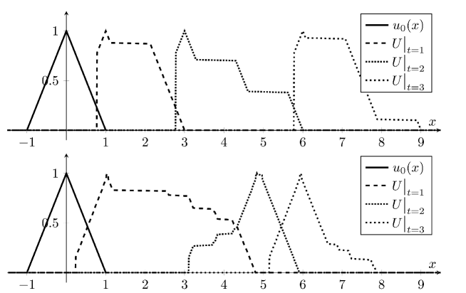
Figure 2: A trajectory of the solution $U(x,t)$ at several time points. Above: The generating Lévy process $X$ is Gamma distributed with scale parameter $k=1$, shape parameter $\theta=1$ and drift $d=1$. Below: The generating Lévy process $X$ is Poisson distributed with jump size 1, intensity $c=1$ and drift $d=1$.

4 Conclusion

A Goupillaud medium is a piecewise constant layered medium such that the thickness of each layer is proportional to the corresponding propagation speed. We have developed a set-up for a specific stochastic Goupillaud medium in which the propagation speeds (or equivalently the thickness of the layers) are given by infinitely divisible random variables. Using a dyadic refinement, these random variables could be constructed as increments of a strictly increasing Lévy process. We have shown that the one-dimensional transport equation can be solved in such a medium, and that the characteristic curves converge to shifted trajectories of the underlying Lévy process as the time step goes to zero. If the initial data are sufficiently regular, the corresponding solutions converge pathwise and in the $p$-th mean to a limiting function, which in addition can be computed by means of a Fourier integral operator.

At this stage, several questions remain open. The first issue is the probability distribution of the limiting characteristic curves $\Gamma(\omega;\tau;x,t)=X\big{(}\omega;\tau+X(\omega)^{*}(x)-t\big{)}$, and subsequently of the limiting solution $U(\omega;t,x)=u_{0}\big{(}\Gamma(\omega;0;x,t)\big{)}$. The second question is how one can give a meaning to the limiting propagation speed $c(x)$ as a (generalized) function of $x$. Given a positive answer to this question, one may finally ask if there is solution concept that would allow one to interpret $U(\omega;t,x)$ as a solution in some sense. All these issues are the subject of ongoing research.

Acknowledgement

The second author acknowledges support through the research project P-27570-N26 “Stochastic generalized Fourier integral operators” of FWF (The Austrian Science Fund). The third author acknowledges support through the Bridge Project No. 846038 “Fourier Integral Operators in Stochastic Structural Analysis” of FFG (The Austrian Research Promotion Agency).

References

- [1] L. Ambrosio. Transport equation and Cauchy problem for vector fields. Invent. Math., 158(2):227–260, 2004.
- [2] L. Ambrosio. Transport equation and Cauchy problem for non-smooth vector fields. In L. Ambrosio, L. Cafarelli, M. G. Crandall, L. C. Evans, and N. Fusco, editors, Calculus of variations and nonlinear partial differential equations, volume 1927 of Lecture Notes in Math., pages 1–41. Springer, Berlin, 2008.
- [3] Patrick Billingsley. Convergence of probability measures. John Wiley & Sons, New York, 2 edition, 1999.
- [4] F. Bouchut and F. James. One-dimensional transport equations with discontinuous coefficients. Nonlinear Anal., 32(7):891–933, 1998.
- [5] R. Burridge, G. S. Papanicolaou, and B. S. White. One-dimensional wave propagation in a highly discontinuous medium. Wave Motion, 10(1):19–44, 1988.
- [6] R. J. DiPerna and P.-L. Lions. Ordinary differential equations, transport theory and Sobolev spaces. Invent. Math., 98(3):511–547, 1989.
- [7] F. Flandoli. Random perturbation of PDEs and fluid dynamic models, volume 2015 of Lecture Notes in Mathematics. Springer, Heidelberg, 2011. Lectures from the 40th Probability Summer School held in Saint-Flour, 2010.
- [8] J.-P. Fouque, J. Garnier, G. Papanicolaou, and K. Sølna. Wave propagation and time reversal in randomly layered media, volume 56 of Stochastic Modelling and Applied Probability. Springer, New York, 2007.
- [9] Roger G. Ghanem and Pol D. Spanos. Stochastic finite elements: a spectral approach. Springer-Verlag, New York, 1991.
- [10] Pierre L. Goupillaud. An approach to inverse filtering of near-surface layer effects from seismic records. Geophysics, 26:754–760, 1961.
- [11] M. Hairer. A theory of regularity structures. Invent. Math., 198(2):269–504, 2014.
- [12] S. Haller and G. Hörmann. Comparison of some solution concepts for linear first-order hyperbolic differential equations with non-smooth coefficients. Publ. Inst. Math. (Beograd) (N.S.), 84(98):123–157, 2008.
- [13] O. Kallenberg. Foundations of modern probability. Probability and its Applications (New York). Springer-Verlag, New York, second edition, 2002.
- [14] Hermann G. Matthies. Stochastic finite elements: computational approaches to stochastic partial differential equations. ZAMM Z. Angew. Math. Mech., 88(11):849–873, 2008.
- [15] B. Nair and B. S. White. High-frequency wave propagation in random media—a unified approach. SIAM J. Appl. Math., 51(2):374–411, 1991.
- [16] M. Oberguggenberger and M. Schwarz. Fourier integral operators in stochastic structural analysis. In F. Werner, M. Huber, T. Lahmer, T. Most, and D. Proske, editors, Proceedings of the 12th International Probabilistic Workshop, volume 11 of Schriftenreihe des DFG Graduiertenkollegs 1462 Modellqualitäten, pages 250–257. Bauhaus-Universitätsverlag, Weimar, 2014.
- [17] S. Pilipović and D. Seleši. On the generalized stochastic Dirichlet problem—Part II: solvability, stability and the Colombeau case. Potential Anal., 33(3):263–289, 2010.
- [18] S. Pilipović and D. Seleši. On the generalized stochastic Dirichlet problem. I. The stochastic weak maximum principle. Potential Anal., 32(4):363–387, 2010.
- [19] Ken-iti Sato. Lévy Processes and Infinitely Divisible Distributions. Cambridge University Press, Cambridge, 1999.