Quantum Feedback Cooling of a Mechanical Oscillator Using Variational Measurements: Tweaking Heisenberg’s Microscope

Abstract

We revisit the problem of preparing a mechanical oscillator in the vicinity of its quantum-mechanical ground state by means of feedback cooling based on continuous optical detection of the oscillator position. In the parameter regime relevant to ground state cooling, the optical back-action and imprecision noise set the bottleneck of achievable cooling and must be carefully balanced. This can be achieved by adapting the phase of the local oscillator in the homodyne detection realizing a so-called variational measurement. The trade-off between accurate position measurement and minimal disturbance can be understood in terms of Heisenberg’s microscope and becomes particularly relevant when the measurement and feedback processes happen to be fast within the quantum coherence time of the system to be cooled. This corresponds to the regime of large quantum cooperativity $C_{\rm{q}}\gtrsim 1$, which was achieved in recent experiments on feedback cooling. Our method provides a simple path to further pushing the limits of current state-of-the-art experiments in quantum optomechanics.

1 Introduction

The task of exerting quantum-level control over the motion of mechanically compliant elements has become a central challenge in several fields of physics ranging from quantum-limited measurement of the motion of kilogram-scale mirrors in laser-interferometric gravitational wave detectors [1, 2] to experiments with nano- and micromechanical oscillators in optomechanics [3, 4]. A paradigmatic example of such a system is an optical cavity mode coupling via radiation pressure to a mechanical mode whose motion modulates the optical resonance frequency (see Fig. 1). Current experiments in this direction involving meso- and microscopic oscillators include implementations of state-transfer [5, 6], frequency conversion [7, 8, 9], impulse force measurement [10], dynamical back-action cooling to near the quantum mechanical ground state [11, 12, 13, 14], ponderomotive squeezing of light [15, 16, 17], and the generation of nonclassical [18], squeezed [19] and entangled states [20] of mechanical oscillators. Of these, the capability to perform ground-state cooling is the most straightforward benchmark of a quantum-enabled system, and it is this task that we will consider in the present paper.

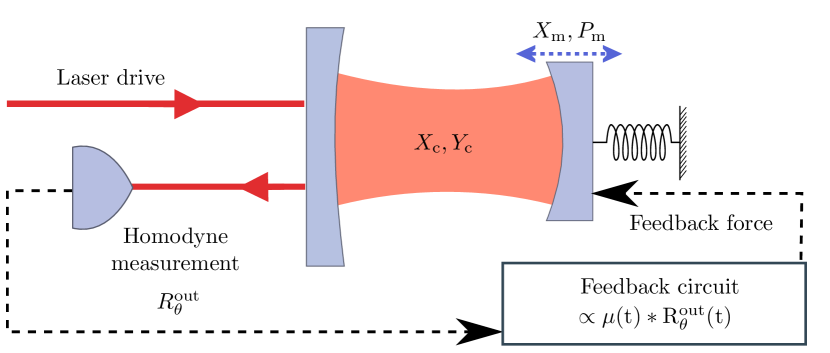
Figure 1: Optomechanical system with feedback. The mechanical motion of the end-mirror in a Fabry-Pérot cavity mirror of position $X_{\rm{m}}$ and momentum $P_{\rm{m}}$ is radiation-pressure coupled to a single cavity mode described by amplitude and phase quadratures $X_{\rm{c}},Y_{\rm{c}}$. The light serves as a meter field, which is continually read out from the cavity, and a particular quadrature $R_{\theta}^{\rm{out}}$ is obtained by homodyne measurement at local oscillator phase $\theta$. Based on the measurement record, that is determined by a spectral gain function $\mu(\rm{t})$ programmed into the feedback circuit, a feedback force is applied to the mechanically compliant mirror ideally steering it into its ground state.

Generally, two main approaches to optomechanical cooling have been considered in the literature, being of respectively passive and active nature: Dynamical back-action cooling and feedback cooling [21]. The former relies on overcoupling the mechanical mode to a “cold” reservoir (e.g. optical vacuum) to which it will equilibrate. Meanwhile, feedback cooling works by continuously measuring the oscillator motion and, conditioned on the result, applying a force to the oscillator by some auxiliary means. In either scheme the cooling can be understood as an attempt to map the state of the quiet meter field onto the mechanical mode faster than the thermal decoherence rate of the latter. Roughly speaking, these approaches are preferred in the resolved- and unresolved-sideband regimes, respectively [21]. Whereas dynamical back-action cooling to the vicinity of the ground state has already been successfully demonstrated in numerous experiments [11, 12, 13, 14], it is only recently that active feedback cooling has started to approach the quantum regime [22, 23]. Reflecting this circumstance, the theory of quantum feedback cooling has not been explored to the same extent as that of the passive approach, and it is here the present work seeks to contribute.

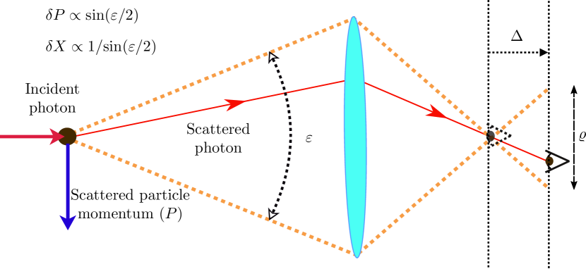
Figure 2: Heisenberg’s microscope modified by using a variational measurement that simultaneously obtains information about position and momentum: A particle (black dot) is confined to the focal plane of the lens (turquoise ellipse). A photon incident from the left scatters off the particle giving it a momentum kick. Photons within the angle $\varepsilon$ are collected by the lens and refocused at the image plane (eye, dashed). In this configuration, the image resolution is set by the diffraction limit of light, $\delta X\propto 1/\sin(\varepsilon/2)$, whereas the uncertainty in momentum introduced by the scattering is $\delta P\propto\sin(\varepsilon/2)$. Moving the observation plane a distance $\Delta$ out of focus decreases the position resolution ($\propto 1/\varrho$) but allow the observer (eye, solid) to partially resolve where in the plane the scattered photon arrived.

In feedback cooling schemes, a balance must be sought between the level of precision at which the system of interest is monitored and the level of disturbance introduced to it. In the context of optomechanics, the measurement imprecision is set by the vacuum fluctuations of the measured field quadrature while measurement back action is due to vacuum fluctuations in the amplitude quadrature. The trade-off between measurement error and disturbance is a familiar theme within the realm of quantum mechanics which is well illustrated by the famous Gedankenexperiment on the Heisenberg microscope (Fig. 2) and is expressed quantitatively in quantum measurement theory in terms of the standard quantum limit for continuous measurements [1] and error-disturbance relations [24]. In the context of feedback cooling, it will be vital to choose the right trade-off between measurement precision and disturbance of the system in order to minimize the effective mechanical temperature. This issue becomes relevant when the measurement and feedback processes happen to be fast compared to the quantum coherence time of the system to be cooled as demonstrated in the recent experiment by Wilson et al. [22, 23]. We note that this is equivalent to the regime of so-called strong optomechanical cooperativity which has been achieved, albeit in other contexts, in several of the experiments cited above. In view of this recent experimental progress we will address here one particular easily-implementable method to balance error and disturbance, namely the adjustment of the local oscillator phase in the homodyne detection of light. This method has been suggested first in the context of gravitational-wave detectors by Vyatchanin [25] and Kimble [26]. It has also been suggested in our specific context of quantum feedback cooling in Refs. [27, 28], where it was shown theoretically to give an advantage over the conventional phase choice for the local oscillator. Here, we will provide a systematic optimization of the scheme, which has not been given so far and, moreover, we put the method in the appropriate conceptual framework of measurement error and disturbance.

In the next section we will introduce a model system for feedback cooling in optomechanics after which we will present its solution in Sec. 3. Before proceeding with the rigorous analysis, we provide in Sec. 4 an intuitive explanation of the error-disturbance balance in feedback cooling and the role of using variational measurements. Then in Secs. 5 and 6 we calculate and minimize the effective mechanical temperature in the presence of variational measurements. Finally, we conclude and give an outlook in Sec. 7.

2 Optomechanical equations of motion with feedback

We will now present the model system to be analyzed. As schematically shown in Fig. 1, we study the standard optomechanical setup consisting of a Fabry-Pérot cavity with a resonating mirror, but the treatment is applicable to other types of optomechanical setups. The optical output from the cavity is sent to a balanced homodyne detector, measuring the optical quadrature $R_{\theta}^{\rm{out}}$ parametrized by the local oscillator (LO) phase $\theta$. The feedback circuit processes the measured signal according to a specified gain function $\mu(t)$ and applies a feedback force ($\propto\mu\left(t\right)*R_{\theta}^{\rm{out}}\left(t\right)$, where $*$ denotes a convolution) on the mechanical oscillator accordingly. We restrict ourselves to feedback that depends linearly on the measurement record, so as to obtain linear effective equations of motion. In particular this accommodates the simulation of a viscous force and hence cooling of the mechanical motion can be engineered.

We seek an effective description of the aforementioned setup including the feedback mechanism. In the limiting case of Markovian feedback ($\mu(t)\propto\delta(t)$) the dynamics can be described by means of the well developed formalism of feedback master equations [29, 30]. Using these methods, Markovian feedback cooling in the regime of strong quantum cooperativity of optomechanics using variational measurement has been explored in [28]. The experimentally more relevant case of Non-Markovian feedback in linear system dynamics is commonly described in the formalism of Heisenberg-Langevin equations which has been fruitfully applied in the context of optomechanics [31, 21]. We will follow this path in the present article. The basic treatment given in this and the next section will largely reproduce the approach of Genes et al. [21].

For our specific purposes of efficient optical readout of the mechanical motion, linear interaction is in fact well suited. The derivation of linear optomechanics from the radiation-pressure Hamiltonian is well-known in the community and here we will largely take the linearized equations as our starting point (see, e.g., Ref. [4] for further details). Essentially, this approach relies on the assumption that the applied laser drive will induce a large intra-cavity field amplitude. Henceforth, we consider the dynamics of the optical and mechanical excursions relative to the corresponding classical steady-state response. We denote these relative coordinates $X_{\rm{m}}$, $P_{\rm{m}}$ for the mechanical position and momentum, and $\delta a$ for the cavity mode amplitude. The linear coupling between these shifted variables of mechanical motion and light field will be enhanced due to the drive, which is essential for performing an efficient optical position measurement. Working in terms of the relative dynamical variables and neglecting nonlinear terms, as they are not enhanced by the strong driving field, the linear Heisenberg-Langevin equations for the fluctuations emerge. Considering resonant readout, where the drive field frequency $\omega_{\rm{d}}$ is aligned with the steady-state cavity resonance, $\omega_{\rm{d}}=\omega_{\rm{c}}$, the Heisenberg-Langevin equations for linear optomechanics including feedback are,

$$\dot{X}_{\rm{m}} = \omega_{\rm{m}}P_{\rm{m}},$$ (1)

$$\dot{P}_{\rm{m}} = -\omega_{\rm{m}}X_{\rm{m}}-\gamma_{\rm{m}}P_{\rm{m}}+g_{\rm{om}}X_{\rm{c}}+\xi+F_{\rm{fb}},$$ (2)

$$\dot{X}_{\rm{c}} = -\frac{\kappa}{2}X_{\rm{c}}+\sqrt{\kappa}X_{\rm{c}}^{\rm{in}},$$ (3)

$$\dot{Y}_{\rm{c}} = -\frac{\kappa}{2}Y_{\rm{c}}+g_{\rm{om}}X_{\rm{m}}+\sqrt{\kappa}Y_{\rm{c}}^{\rm{in}},$$ (4)

where the optical annihilation operator $\delta a$ is replaced by cavity amplitude and phase quadratures in an appropriate rotating frame, $X_{\rm{c}}=(e^{i\omega_{\rm{c}}t}\delta a+e^{-i\omega_{\rm{c}}t}\delta a^{\dagger})/\sqrt{2}$ and $Y_{\rm{c}}=(e^{i\omega_{\rm{c}}t}\delta a-e^{-i\omega_{\rm{c}}t}\delta a^{\dagger})/i\sqrt{2}$. Eqs. (1,2) represent the mechanical oscillator of resonance frequency $\omega_{\rm{m}}$ and intrinsic damping rate $\gamma_{\rm{m}}$, whereas Eqs. (3,4) describe an optical cavity mode which is read out at a rate $\kappa$ (intrinsic cavity damping is equivalent to an imperfect detection efficiency, which will be introduced later). The coupling between these two subsystems is characterized by the optomechanical coupling rate $g_{\rm{om}}=\sqrt{\hbar/m\omega_{\rm{m}}}(d\omega_{\rm{c}}/dx_{\rm{m}})\sqrt{2\Phi_{\rm{in}}/\kappa}$, where $\Phi_{\rm{in}}$ is the photon flux impinging on the cavity, $m$ is the effective mass of the mechanical mode and $(d\omega_{\rm{c}}/dx_{\rm{m}})$ is the optical frequency shift per mechanical displacement. Hence, the coupling rate $g_{\rm{om}}$ can be tuned via $\Phi_{\rm{in}}$ by changing the laser drive power. Note that the Eqs. (3,4) for the optical quadratures are decoupled from one another due to the choice of on-resonant driving, $\omega_{\rm{d}}=\omega_{\rm{c}}$. In this case the mechanical motion is seen to be read out exclusively into the phase quadrature, $Y_{\rm{c}}$, while the back-action force on the mechanical mode, $g_{\rm{om}}X_{\rm{c}}$, comes entirely from the amplitude fluctuations, $X_{\rm{c}}^{\rm{in}}$, as follows from Eq. (3).

We now comment on the source terms in Eqs. (2-4) driving the mechanical and optical modes. The feedback force on the mechanical oscillator is represented by the operator $F_{\rm{fb}}$ appearing in Eq. (2), and we will return to this below. Meanwhile, the thermal noise due to intrinsic mechanical damping, represented by the Langevin operator $\xi$, can for our purposes be characterized in the high-temperature limit $k_{\rm{B}}T\gg\hbar\omega$ by the following correlation function,

$$\left\langle\xi\left(t\right)\xi\left(t^{\prime}\right)\right\rangle\approx\gamma_{\rm{m}}(2\bar{n}+1)\delta\left(t-t^{\prime}\right)$$ (5)

$$\bar{n}\approx k_{\rm{B}}T/\hbar\omega_{\rm{m}},$$ (6)

where $\bar{n}$ is the mean number of phonons in the mechanical oscillator in thermal equilibrium (see Ref. [32] for a discussion of the limitations of this approximation). Turning to the optical subsystem, we assume the optical amplitude and phase inputs $X_{\rm{c}}^{\rm{in}},Y_{\rm{c}}^{\rm{in}}$ to represent vacuum fluctuations, i.e., that these operators have the thermal expectation values

$$\left\langle X_{\rm{c}}^{\rm{in}}\left(t\right)X_{\rm{c}}^{\rm{in}}\left(t^{\prime}\right)\right\rangle =\left\langle Y_{\rm{c}}^{\rm{in}}\left(t\right)Y_{\rm{c}}^{\rm{in}}\left(t^{\prime}\right)\right\rangle$$

$$=(1/2)\delta\left(t-t^{\prime}\right).$$

To describe the optical readout, we must consider the input-output relations of the cavity output field,

$$X_{\rm{c}}^{\rm{out}} = \sqrt{\kappa}X_{\rm{c}}-X_{\rm{c}}^{\rm{in}}$$

$$Y_{\rm{c}}^{\rm{out}} = \sqrt{\kappa}Y_{\rm{c}}-Y{}_{\rm{c}}^{\rm{in}}.$$ (8)

By adjusting the phase of the local oscillator $\theta$ we will be able to combine the amplitude and phase quadratures in different ratios with the aim of better balancing measurement error and disturbance. By considering a general quadrature,

$$R_{\rm{\theta}}^{\rm{out}(in)}\equiv\cos\theta X_{\rm{c}}^{\rm{out}(\rm{in})}+\sin\theta Y_{\rm{c}}^{\rm{out}(\rm{in})},$$

the corresponding input-output relation reads

$$R_{\theta}^{\rm{out}}=\sqrt{\eta}(\sqrt{\kappa}R_{\theta}-R_{\theta}^{\rm{in}})-\sqrt{1-\eta}R_{\theta}^{v},$$ (9)

where we are accounting for internal cavity loss and measurement imperfection by a net measurement efficiency $\eta$, assumed to admix a vacuum field $R^{v}$ that is uncorrelated with $R_{\rm{c}}^{\rm{in}}$. Solving Eqs. (3,4) in the Fourier domain by using the convention $F\left(t\right)=\frac{1}{2\pi}\int_{-\infty}^{+\infty}f\left(\omega\right)e^{-i\omega t}d\omega$, we obtain

$$R_{\theta}\left(\omega\right)=\frac{\sqrt{\kappa}}{\kappa/2-i\omega}R_{\theta}^{{\rm in}}\left(\omega\right)+\frac{\sin\theta\,g_{{\rm om}}}{\kappa/2-i\omega}X_{{\rm m}}\left(\omega\right),$$ (10)

so that by substituting this into Eq. (9), the general output quadrature reads

$$R_{\theta}^{\rm{out}}\left(\omega\right)= \sqrt{\eta}\sin\theta\frac{\sqrt{\kappa}g_{{\rm om}}}{\kappa/2-i\omega}X_{{\rm m}}\left(\omega\right)$$ (11)

$$+\sqrt{\eta}\frac{\kappa/2+i\omega}{\kappa/2-i\omega}R_{\theta}^{\rm{in}}\left(\omega\right)-\sqrt{1-\eta}R_{\theta}^{v}\left(\omega\right).$$

making manifest the readout of the position of resonator $X_{{\rm m}}$, whereas the other terms show the contribution due to measurement noise. Ignoring the dependence on the parameters of the homodyne measurement $\theta$ and $\eta$, the maximal rate at which the mechanical motion $X_{{\rm m}}$ can be mapped to the optical quadrature $R_{\theta}^{{\rm out}}$ is given by the ideal measurement rate,

$$\Gamma_{{\rm meas}}=\frac{4g_{{\rm om}}^{2}}{\kappa},$$ (12)

which in the bad-cavity limit is the square of the coefficient mapping the mechanical oscillator position into the optical readout in (11) for $\eta=1$ and $\theta=\pi/2$. For other values of $\eta,\theta$, the effective readout rate is reduced by a factor of $\eta\sin^{2}\theta$.

Finally, we address the relationship between the feedback force $F_{\mathrm{fb}}$ and the optical homodyne measurement of $R_{\rm{\theta}}^{\rm{out}}$. The feedback circuit integrates the measured quadrature signal up to the present time $t$. Since we are interested in preserving the linearity of the equations of motion, (1-4), we take the feedback force to be given by a temporal convolution

$$F_{\rm{fb}}(t)=-\int_{-\infty}^{t}ds\mu(t-s)R_{\theta}^{\rm{est}}(s),$$ (13)

where $\mu\left(\tau\right)=\mathcal{F}^{-1}\{\mu(\omega)\}$ is the inverse Fourier transform of the spectral gain function, $\mu(\omega)$, and

$$R_{\theta}^{\rm{est}}\equiv\frac{R_{\rm{\theta}}^{\rm{out}}}{\sqrt{\kappa\eta}\sin\theta}=\frac{1}{\sqrt{\kappa\eta}}(\cot\theta X_{\rm{c}}^{\rm{out}}+Y_{\rm{c}}^{\rm{out}})$$ (14)

is the rescaled measurement quadrature. The local oscillator phase $\theta$ in the homodyne measurement selects which light quadrature to condition the feedback force on, as was mentioned above. That we convolve with $R_{\theta}^{\rm{est}}$ in Eq. (13) rather than with the original $R_{\theta}^{\rm{out}}$ of Eq. (9) amounts to a scaling convention for the gain function $\mu(t)$. The convention used here is designed to remove the terms which are related to the measurement apparatus ($\sqrt{\eta}\sin\theta$) from the proportionality factor in the relationship $R_{\rm{\theta}}^{\rm{out}}\propto X_{\rm{m}}$ in Eq. (11). To be clear, $\mu(t)$ is the gain applied after having corrected for the measurement inefficiency $\eta$ and the quadrature angle entering as $\sin\theta$. This choice allows us to vary $\theta$ while keeping fixed the net gain of the position component of the measurement, in turn, keeping the feedback-induced damping fixed as we will see below.

3 Mechanical response and effective susceptibility

Having established the equations of motion (1-4) and the relevant optical input-output relation (11), we turn to solving this set of equations for the mechanical response. Since the system is linear, this is straightforwardly done in the Fourier domain. A useful way of expressing the solution for the mechanical mode is the response relation (suppressing the $\omega$ dependence of the source terms for brevity)

$$X_{\rm{m}}\left(\omega\right)=\chi_{\rm{eff}}(\omega)[\xi+f_{\rm{ba}}+f_{\rm{fb}}+f_{v}],$$ (15)

where the effective mechanical susceptibility is

$$\chi_{\rm{eff}}^{-1}(\omega)=\frac{1}{\omega_{\rm{m}}}[\omega_{\rm{m}}^{2}-\omega^{2}-i\gamma_{\rm{m}}\omega+\mu(\omega)\frac{g_{\rm{om}}\omega_{\rm{m}}}{\kappa/2-i\omega}],$$ (16)

and the four stochastic forces driving the oscillator are the thermal Langevin operator $\xi$ and the fluctuation associated with back-action, feedback, and extraneous vacuum:

$$f_{\rm{ba}}(\omega)=\frac{\sqrt{\kappa}g_{\rm{om}}}{\kappa/2-i\omega}X_{\rm{c}}^{\rm{in}}(\omega),$$ (17)

$$f_{\rm{fb}}(\omega)=-\frac{\kappa/2+i\omega}{\kappa/2-i\omega}\frac{\mu(\omega)}{\sqrt{\kappa}}\left[\cot\theta X_{\rm{c}}^{\rm{in}}(\omega)+Y_{\rm{c}}^{\rm{in}}(\omega)\right],$$ (18)

$$f_{v}(\omega)=\frac{\mu(\omega)}{\sqrt{\kappa}}\sqrt{\eta^{-1}-1}\left[\cot\theta X^{v}(\omega)+Y^{v}(\omega)\right].$$ (19)

The back-action force $f_{\rm{ba}}$ arises from the optical amplitude fluctuations $X_{\rm{c}}^{\rm{in}}$, whereas the noise of the meter field $f_{\rm{fb}}$ introduced via the feedback force contains both optical amplitude and phase fluctuations, $X_{\rm{c}}^{\rm{in}}$ and $Y_{\rm{c}}^{\rm{in}}$, whereby $f_{\rm{ba}}$ and $f_{\rm{fb}}$ are correlated (for general $\theta$). $f_{v}$ is the part of the feedback force fluctuations coming from extraneous vacuum noise due to optical losses.

We see that the feedback gain function $\mu(\omega)$, i.e. the Fourier transform of $\mu(\tau)$, enters in the effective mechanical susceptibility $\chi_{\rm{eff}}$ as well as $f_{\rm{fb}}$ and $f_{v}$, Eqs. (16,18,19). The choice of the function $\mu(\omega)$ can hence be thought of as influencing both the response characteristics and the spectral mapping of imprecision noise into the oscillator. Following Ref. [21] we choose the gain function

$$\mu(t)=\mu_{\rm{fb}}\frac{d}{dt}[\Theta(t)\omega_{\rm{fb}}e^{-t\omega_{\rm{fb}}}],$$ (20)

which in the frequency domain becomes

$$\mu(\omega)=\frac{-i\omega\mu_{\rm{fb}}}{1-i\frac{\omega}{\omega_{\rm{fb}}}},$$ (21)

where $\mu_{\rm{fb}}$ is the dimensionless feedback gain, $\omega_{\rm{fb}}$ is a low-pass cut-off frequency, and $\Theta(t)$ is the Heaviside function. Considering Eq. (21) in the limit $\omega_{\rm{fb}}\rightarrow\infty$, we see that it corresponds to a time derivative of the measurement current. The rationale behind this choice is to achieve an effective friction force ($F_{fb}\propto-P_{m}\propto-\dot{X}_{m}$) which is attained through the time derivative of the photocurrent given the fact that light reads out the position of the mechanical oscillator. For finite $\omega_{\rm{fb}}$, we can then think of the feedback filter as performing a derivative combined with a low-pass filter. Note, however, that the value of $\omega_{\rm{fb}}$ not only controls the frequency-cutoff of $|\mu(\omega)|$, but also influences the feedback phase function $\rm{Arg}[\mu(\omega)]$. By considering Eq. (16) for this choice of feedback function, Eq. (21), we can extract the effective mechanical resonance frequency and dissipation rate. In the bad-cavity limit we find

$$\omega_{\rm{eff,m}}(\omega) = \sqrt{\omega_{\rm{m}}^{2}+\frac{\sigma\gamma_{\rm{m}}\omega_{\rm{fb}}\omega^{2}}{\omega_{\rm{fb}}^{2}+\omega^{2}}},$$ (22)

$$\gamma_{\rm{eff,m}}(\omega) = \gamma_{\rm{m}}\left(1+\frac{\sigma\omega_{\rm{fb}}^{2}}{\omega_{\rm{fb}}^{2}+\omega^{2}}\right),$$ (23)

$$\chi_{\rm{eff}}^{-1}(\omega) = \frac{1}{\omega_{\rm{m}}}[\omega_{\rm{eff,m}}^{2}(\omega)-\omega^{2}-i\gamma_{\rm{eff,m}}(\omega)\omega],$$ (24)

where

$$\sigma\equiv\frac{2\mu_{\rm{fb}}g_{\rm{om}}\omega_{\rm{m}}}{\kappa\gamma_{\rm{m}}}$$ (25)

is the rescaled dimensionless feedback gain. More precisely, then, we define the bad-cavity limit as $\kappa\rightarrow\infty$ while keeping $\sigma$ and $\Gamma_{{\rm meas}}$ finite. Practical considerations may limit the available range of the absolute feedback gain $\tilde{\sigma}=\sigma/(\sqrt{\kappa\eta}\sin\theta)$, cf. Eqs. (13,14). Deviation from $\eta=1$ and $\theta=\pi/2$ requires larger absolute gain $\tilde{\sigma}$ in order to maintain a certain value of $\sigma$, the gain parameter entering $\chi_{\rm{eff}}(\omega)$. The stability of the optomechanical system in the presence of feedback can be determined from the complex poles of $\chi_{\rm{eff}}(\omega)$ using the Routh-Hurwitz criterion [33]. Here it suffices to remark that in the idealized bad-cavity limit considered here, $\kappa\rightarrow\infty$, the stability criterion is fulfilled for all values of $\sigma$. (We give the stability criterion for arbitrary values of $\kappa$ in A.)

4 Variational measurements and Heisenberg’s microscope

Before calculating the mechanical steady-state occupation from the solution found in the preceding section, it is appropriate to pause for a more qualitative discussion of the physics that will emerge from the analysis. At a very basic level, the idea of feedback cooling of a mechanical oscillator is simply that if we monitor its motion (by means of some meter degree of freedom), we may, based on this information, apply an effectively viscous force, that will dampen the motion. The extent to which we are able to bring the motion to a halt by this technique will be determined by the interplay of (at least) four effects as seen from Eq. (15): Firstly, the thermal noise, $\xi$, driving the motion due to the internal friction mechanisms of the mechanical element. Secondly, the disturbing back-action force, $f_{\rm{ba}}$, of the meter system on the mechanical motion, e.g., the radiation-pressure shot noise arising from the random timing of the momentum kicks imparted on the mechanical oscillator by the impinging photons. Thirdly, the imprecision noise, $f_{\rm{fb}}$, of the position measurement, which limits the ability to apply the right amount of force required to halt the motion. Fourthly, the feedback modification of the mechanical response function, $\chi_{\rm{eff}},$ by inducing an increased damping.

In considering how to balance these effects, it is important to acknowledge the time-continuous nature of the scheme: For instance, if we were to attempt a perfectly precise instantaneous position measurement, the back-action force would introduce a large uncertainty in the mechanical momentum, as per Heisenberg’s uncertainty relation, rendering the position a short while later completely unpredictable. If, on the other hand, we were to measure very weakly to avoid disturbing the system, the imprecision noise would dominate and very little information would be gained. Both outcomes are clearly at odds with the desired goal of cooling and we are therefore led to strike a balance between the influences of back-action and imprecision noise. In terms of the Gedankenexperiment of Heisenberg’s microscope, this trade-off would correspond to sacrificing (instantaneous) position resolution to gain increased information about the direction of the scattered photon (see Fig. 2). The possibility of further optimizing feedback cooling in this way has previously been pointed out in Ref. [27], although without extensive analysis or discussion. In the remainder of this section, we will provide intuition as to why variational measurements can be advantageous.

While we must generally include the thermal influence of intrinsic mechanical damping in the analysis (and will do so below), the main interest of this work is the regime of quantum operation, where this thermal load is perturbative. To establish intuition that will be useful in interpreting the results of the rigorous analysis to be presented in subsequent sections, we therefore proceed now to consider the trade-off between back-action and imprecision noise. This simpler scenario, in which we only consider the fundamental fluctuations required by quantum mechanics, is only adequate to the extent that the measurement and feedback processes occur fast compared to the thermal coherence time $\sim 1/\gamma_{\rm{m}}\bar{n}$. This is the limit of very large quantum cooperativity,

$$C_{\rm{q}}\equiv\frac{\Gamma_{\rm{meas}}}{\gamma_{\rm{m}}\bar{n}}=\frac{4g_{\rm{om}}^{2}}{\kappa\gamma_{\rm{m}}\bar{n}}\gg 1,$$

and fast feedback $\sigma\propto\Gamma_{\rm{meas}}/\gamma_{\rm m}$ (whereas in current state-of-the-art experiments, $C_{\rm{q}}\gtrsim 1$). In this limit we may for the purposes of the present discussion take the mechanical response, (15), to be (in the bad-cavity limit and assuming perfect detection, $\eta=1$)

$$X_{\rm{m}}(\omega) =\chi_{\rm{eff}}(\omega)F(\omega)$$ (26)

$$F(\omega) \approx f_{\rm{ba}}(\omega)+f_{\rm{fb}}(\omega)$$ (27)

$$=\left[\sqrt{\Gamma}_{\rm meas}-\frac{\mu(\omega)}{\sqrt{\kappa}}\cot\theta\right]X_{\rm{c}}^{\rm{in}}(\omega)$$

$$-\frac{\mu(\omega)}{\sqrt{\kappa}}Y_{\rm{c}}^{\rm{in}}(\omega),$$

where the expression for the force $F(\omega)$ is organized according to its contributions from amplitude and phase fluctuations. Eq. (27) emphasizes the fact that for general $\theta$ the amplitude fluctuations drive the mechanical motion both directly, via the back-action force $f_{\rm{ba}}$, and indirectly, via the fluctuations $f_{\rm{fb}}$ injected by the feedback mechanism. As these contributions add coherently in determining the mechanical response, the possibility of destructive interference arises. Moreover, Eq. (27) shows that the interference varies with $\omega$. This dependence must be considered over the effective mechanical bandwidth, which is typically set by the feedback-induced broadening, Eq. (23). This observation hints at a trade-off between, on the one hand, achieving favorable interference over the entire effective bandwidth and, on the other hand, suppressing thermal noise by applying a large feedback gain.

Having established the interference effect between back-action and feedback forces, we now turn to the question of what constitutes favorable interference and, in particular, how $\theta$ and $\mu(\omega)$ should be chosen to attain this. In the classical regime, where thermal noise dominates, back-action noise can be neglected and the optimal measurement quadrature is the phase quadrature ($\theta=\pi/2$), into which the position measurement is read out (as described in Sec. 2). In the quantum regime this is no longer the case as can be demonstrated by a simple geometrical argument, that we will now turn to. Since the purpose of the scheme is to map the vacuum state of light onto the mechanical mode, as mentioned previously, the scheme can only be successful if the (orthogonal) noise quadratures of light $X_{\rm{c}}^{\rm{in}},Y_{\rm{c}}^{\rm{in}}$ are mapped to orthogonal mechanical quadratures with equal strength. If this were not the case, it would violate equipartition between the mechanical quadratures and thus the resulting mechanical state could impossibly be the ground state. To understand the mapping into $X_{\rm{m}}$ and $P_{\rm{m}}$, we note that the Fourier transform of Eq. (1) is $P_{\rm{m}}(\omega)=-i(\omega/\omega_{\rm{m}})X_{\rm{m}}(\omega)$. The relative phase of $(-i)$ between the position and momentum response entails that the real and imaginary parts of $X_{\rm{m}}(\omega)=\chi_{\rm{eff}}(\omega)F(\omega)$, which are $X_{\rm{m}}(\omega)+X_{\rm{m}}^{\dagger}(\omega)$ and $[X_{\rm{m}}(\omega)-X_{\rm{m}}^{\dagger}(\omega)]/i$, will map to orthogonal mechanical quadratures as seen from the time-domain response (in a narrow-band approximation for simplicity)

$$X_{\rm{m}}(t) \propto \left(e^{-i\omega_{\rm{m}}t}X_{\rm{m}}(\omega_{\rm{m}})+\rm{H.c.}\right)$$ (28)

$$= \cos(\omega_{\rm{m}}t)\left[X_{\rm{m}}(\omega_{\rm{m}})+X_{\rm{m}}^{\dagger}(\omega_{\rm{m}})\right]$$

$$+\sin(\omega_{\rm{m}}t)\left[X_{\rm{m}}(\omega_{\rm{m}})-X_{\rm{m}}^{\dagger}(\omega_{\rm{m}})\right]/i$$

$$P_{\rm{m}}(t) \propto \left(e^{-i\omega_{\rm{m}}t}P_{\rm{m}}(\omega_{\rm{m}})+\rm{H.c.}\right)$$ (29)

$$\approx \cos(\omega_{\rm{m}}t)\left[X_{\rm{m}}(\omega_{\rm{m}})-X_{\rm{m}}^{\dagger}(\omega_{\rm{m}})\right]/i$$

$$-\sin(\omega_{\rm{m}}t)\left[X_{\rm{m}}(\omega_{\rm{m}})+X_{\rm{m}}^{\dagger}(\omega_{\rm{m}})\right].$$

Thus, the above equipartition argument requires $X_{\rm{m}}(\omega_{\rm{m}})+X_{\rm{m}}^{\dagger}(\omega_{\rm{m}})$ and $[X_{\rm{m}}(\omega_{\rm{m}})-X_{\rm{m}}^{\dagger}(\omega_{\rm{m}})]/i$ to represent orthogonal quadratures of light with equal weight.

Let us now apply this mapping condition to Eqs. (26,27) near resonance $\omega\approx\omega_{\rm{m}}$. We introduce the simplified symbols $a\equiv\sqrt{\Gamma}_{\rm meas}$, $b\equiv|\mu(\omega_{\rm{m}})/\sqrt{\kappa}|,$ and $\phi=\rm{Arg}[-\mu(\omega_{\rm{m}})/\sqrt{\kappa}]$, whereby the force, (27), can be expressed as

$$F(\omega)=(a+be^{i\phi}\cot\theta)X_{\rm{c}}^{\rm{in}}\left(\omega\right)+be^{i\phi}Y_{\rm{c}}^{\rm{in}}\left(\omega\right).$$ (30)

We now fix $a$ and consider two characteristic values of $\phi$ (see Fig. 3): For $\phi=\pi/2$, $f_{\rm{ba}}$ and $f_{\rm{fb}}$ add in quadrature and we see from (30) that matching can only be achieved for $\theta=\pi/2$ and $b=a$ as illustrated in Fig. 3a. Consider now the case of $\phi=3\pi/4$, whereby part of $f_{\rm{fb}}$ is anti-correlated with $f_{\rm{ba}}$ and matching can be achieved by choosing $\theta=\pi/4$ and $b=a/\sqrt{2}$ (Fig. 3b). In the second scenario, part of the direct back action is cancelled by partially measuring the amplitude fluctuations in the light field and feeding them back into the mechanical mode via the feedback force, while operating at the same absolute feedback gain $\propto b/\sin\theta$ as in the first scenario (with $\theta=\pi/2$). Hence the second scenario leads to less fluctuations in the mechanical mode and thus the resulting state will be closer to the ground state as will in fact be found in the rigorous analysis below. These simple considerations indicate that in the quantum regime it is important to properly choose both the homodyne measurement quadrature, via $\theta$, and the feedback gain $\mu(\omega)$. Note however, as remarked below Eq. (27), that the matching consideration illustrated in Fig. 3 should be applied to all frequencies within the effective mechanical bandwidth. Since our chosen value of $\theta$ is a constant, whereas the feedback gain $\mu(\omega)$ is frequency dependent, it will in general not be possible to achieve advantageous interference over the entire bandwidth. In the next section we resume the quantitative mathematical analysis.

Figure 3: Geometrical considerations regarding the choice of homodyne quadrature angle $\theta$. Depicted are the mapping coefficients of $X_{\rm{c}}^{\rm{in}}(\omega),Y_{\rm{c}}^{\rm{in}}(\omega)$ in (30) as solid arrows in the complex plane. Two cases are considered: a) $\phi=\pi/2,\theta=\pi/2,b=a$; b) $\phi=3\pi/4,\theta=\pi/4,b=a/\sqrt{2}$.

5 Steady-state occupation in the bad-cavity regime

Given the solution (15) for the spectral response of the mechanical mode, we are now in a position to calculate the average number of phonons $n_{\rm{tot}}$ it contains in the steady state of the feedback scheme. This quantity will serve as our figure of merit, with $n_{\rm{tot}}<1$ being the regime of interest. By considering the Hamiltonian of the free mechanical oscillator,

$$H=\frac{\hbar\omega_{\rm{m}}}{2}\left(X_{\rm{m}}^{2}+P_{\rm{m}}^{2}\right)=\hbar\omega_{\rm{m}}\left(\hat{n}_{\rm{tot}}+\frac{1}{2}\right),$$ (31)

which is stated in terms of the variance of the dimensionless operators $X_{\rm{m}}$ and $P_{\rm{m}}$, we can extract the mean number of phonons ${n}_{\rm{tot}}=\langle\hat{n}_{\rm{tot}}\rangle$ as an integral over spectral density of each quadrature,

$$n_{\rm{tot}}=\frac{1}{2}\int_{-\infty}^{\infty}\frac{d\omega}{2\pi}\left(S_{X}\left(\omega\right)+S_{P}\left(\omega\right)\right)-\frac{1}{2},$$ (32)

where we have introduced the position and momentum fluctuation spectra

$$S_{X}\left(\omega\right) = \int_{-\infty}^{\infty}d\omega^{\prime}\left\langle X_{\rm{m}}\left(\omega\right)X_{\rm{m}}\left(\omega^{\prime}\right)\right\rangle,$$ (33)

$$S_{P}\left(\omega\right) = \int_{-\infty}^{\infty}d\omega^{\prime}\left\langle P_{\rm{m}}\left(\omega\right)P_{\rm{m}}\left(\omega^{\prime}\right)\right\rangle.$$ (34)

Using Eq. (15) the position spectrum reads

$$S_{X}\left(\omega\right)= \int_{-\infty}^{\infty}d\omega^{\prime}|\chi_{\rm{eff}}(\omega)|^{2}\bigg{(}\left\langle\xi(\omega)\xi(\omega^{\prime})\right\rangle$$ (35)

$$+\left\langle f_{\rm{ba}}(\omega)f_{\rm{ba}}(\omega^{\prime})\right\rangle+\left\langle f_{\rm{fb}}(\omega)f_{\rm{fb}}(\omega^{\prime})\right\rangle$$

$$+\left\langle f_{\rm{co}}(\omega)f_{\rm{co}}(\omega^{\prime})\right\rangle+\left\langle f_{v}(\omega)f_{v}(\omega^{\prime})\right\rangle\bigg{)},$$

where

$$\left\langle f_{\rm{co}}(\omega)f_{\rm{co}}(\omega^{\prime})\right\rangle\equiv\left\langle f_{\rm{fb}}\left(\omega\right)f_{\rm{ba}}\left(\omega^{\prime}\right)+f_{\rm{ba}}\left(\omega\right)f_{\rm{fb}}\left(\omega^{\prime}\right)\right\rangle$$ (36)

is the correlation between back-action noise and feedback force. As discussed in Sec. 4, the indirect back action, coming through the feedback force, is responsible for this cross correlation. As one can easily find by using the Fourier transform of Eq. (1), we use the relation $S_{P}=\omega^{2}S_{X}/\omega_{\rm m}^{2}$ to simplify the calculation of Eq. (32). The correlation functions appearing on the right-hand side of Eq. (35) can be determined from the definitions in Eqs. (17-19) by using appropriate Fourier domain equivalents of Eqs. (5-LABEL:eq:vacuum-correl). By performing the integral (32) (using the analytical procedure given in C) we obtain an expression of the form

$$n_{\rm{tot}}=n_{\rm{th}}+n_{\rm{ba}}+n_{\rm{fb}}+n_{\rm{co}}+n_{v}-\frac{1}{2},$$ (37)

where the various contributions correspond to the respective terms in Eq. (35). The clear physical origin of these terms aids the interpretation of their impact on the total occupation number. The cross-correlation between direct back-action and the feedback noise is represented by $n_{\rm{co}}$, which for parameters of interest is negative.

Since feedback cooling is typically applied in the bad-cavity regime, $\kappa\gg\omega_{\rm{m}},\omega_{\rm{fb}}$, we will henceforth focus on this parameter regime for simplicity of analysis (see the B for a general expression for $n_{\rm{tot}}$ valid for all values of $\kappa$). We parametrize the feedback cut-off frequency $\omega_{\rm{fb}}$ by its ratio to the mechanical resonance frequency

$$\alpha\equiv\omega_{\rm{fb}}/\omega_{\rm{m}},$$ (38)

and note that $\alpha$ is typically within an order of magnitude of unity. Introducing the mechanical quality factor $Q_{\rm{m}}\equiv\omega_{\rm{m}}/\gamma_{\rm{m}}$, for which values on the order of $10^{6}$ and beyond are routinely achieved in optomechanical experiments, we can therefore safely make the additional assumption that $Q_{\rm{m}}\gg\alpha,\alpha^{-1}$. Under these assumptions the various contributions to $n_{\rm{tot}}$ (37) are evaluated to

$$n_{\rm{th}} = \frac{1}{D}\left(\overline{n}+\frac{1}{2}\right)\left(1+\alpha^{-2}+\frac{1}{\alpha}\frac{\sigma}{2Q_{\rm{m}}}\right),$$ (39)

$$n_{\rm{ba}} = \frac{C_{\rm{cl}}}{4D}\left(1+\alpha^{-2}+\frac{1}{\alpha}\frac{\sigma}{2Q_{\rm{m}}}\right),$$ (40)

$$n_{\rm{fb}} = \frac{\sigma^{2}}{4C_{\rm{cl}}D}\left(1+\alpha\frac{\sigma}{2Q_{\rm{m}}}\right)\csc^{2}\left(\theta\right),$$ (41)

$$n_{\rm{co}} = -\frac{\sigma}{2\alpha D}\left(1+\alpha\frac{\sigma}{2Q_{\rm{m}}}\right)\cot\left(\theta\right),$$ (42)

$$n_{v} = n_{\rm{fb}}\left(\eta^{-1}-1\right),$$ (43)

$$D \equiv 1+\sigma+\alpha^{-2},$$ (44)

where

$$C_{\rm{cl}}\equiv 4g_{\rm{om}}^{2}/\kappa\gamma_{\rm{m}}$$ (45)

is the classical cooperativity.

These results are relatively simple and we will now discuss their behavior. We start by noting that the feedback-induced mechanical broadening (23) is given by $\gamma_{\rm{m,eff}}(\omega_{\rm{m}})-\gamma_{\rm{m}}=\sigma/[1+\alpha^{-2}]$, within a narrow-band approximation $\omega\approx\omega_{m}$. This increased broadening will tend to decouple the mechanical mode from its thermal bath while adding low-temperature noise from the optical bath resulting in net cooling, as is seen by considering the behavior of $n_{\rm{th}}$ (39) with increasing $\sigma$. However, this only holds insofar as the scaled cut-off feedback frequency $\alpha$ is large enough for the feedback mechanism to be able to react on the appropriate timescale. Moreover, there is a limit to how much $n_{\rm{th}}$ can be suppressed in this way which manifests itself when the effective mechanical quality factor becomes too small, $Q_{\rm{m,eff}}\equiv\omega_{\rm{m}}/\gamma_{\rm{m,eff}}\ll\alpha,\alpha^{-1}$, as can be seen by taking the limit $\sigma\rightarrow\infty$. Since we treat both the thermal noise and the back-action as white noise (given the lack of cavity filtering in the bad cavity regime), Eqs. (39,40) are seen to be very similar, with $C_{\rm{cl}}/4$ simply playing the role of $\bar{n}+1/2,$ i.e. an equivalent back-action noise flux per unit bandwidth.

We now turn to the imprecision noise contribution $n_{\rm{fb}}$, (41). The increase in $n_{\rm{fb}}$ seen when $\theta$ moves away from $\pi/2$ occurs because this degrades the signal-to-noise ratio of the homodyne measurement. Unsurprisingly, $n_{\rm{fb}}$ increases with scaled effective gain $\sigma$, in fact it diverges as expected from amplifying a noisy measurement excessively. Interestingly, $n_{\rm{fb}}$ also diverges for $\alpha\rightarrow\infty$, i.e., when taking the feedback frequency cut-off $\omega_{\rm{fb}}$ to infinity which yields a derivative filter, see Eq. (21). While this is ideal from the point of view of estimating the instantaneous mechanical velocity, it simultaneously feeds amplified imprecision noise into the oscillator from an unbounded spectral range resulting in $n_{\rm{fb}}\rightarrow\infty$ (as $\alpha\rightarrow\infty$). This observation prompts us to choose values of $\alpha$ which are not too large, which runs counter to the demand of having a large $\alpha$ to be able to cool out the mechanical noise. Hence the finite optimal value for $\alpha$ somehow balances these considerations. Imperfect homodyne detection or optical losses inject additional (uncorrelated) vacuum noise into the measurement current as accounted for by $n_{v}$, Eq. (43).

The novel aspect of the present work hinges on the fact that for a general homodyne quadrature $\theta$, the imprecision shot noise of the measurement is correlated with the back-action noise on the mechanical mode as discussed previously. If we have anti-correlations, $n_{\rm{co}}<0$, destructive interference lessens the total mechanical occupancy $n_{\rm{tot}}$ potentially leading to an advantage over the conventional choice of $\theta=\pi/2$ that maximizes the signal-to-noise ratio of the measurement. Since the dependence of $n_{\rm{tot}}$ on $\theta$ is just that of Eqs. (41-43), the value of $\theta_{\rm{opt}}$ which minimizes $n_{\rm{tot}}$ is straightforwardly found to be

$$\theta_{\rm{opt}}=\rm{Arccot}\left(\frac{\it{C}_{\rm{cl}}\eta}{\alpha\sigma}\right).$$ (46)

Substituting $\theta=\theta_{\rm{opt}}$ back into Eqs. (41,42) and summing all contributions according to (37), we find,

$$\left.n_{\rm{tot}}\right|_{\theta_{\rm{opt}}}=-\frac{1}{2}+\left(1+\sigma+\alpha^{-2}\right)^{-1}\times$$

$$\Bigg{[}\left(\overline{n}+\frac{1}{2}+\frac{C_{\rm{cl}}}{4}\right)\left(1+\alpha^{-2}+\frac{1}{\alpha}\frac{\sigma}{2Q_{\rm{m}}}\right)$$

$$+\left(\frac{\sigma^{2}}{4C_{\rm{cl}}\eta}-\frac{C_{\rm{cl}}\eta}{4\alpha^{2}}\right)\left(1+\alpha\frac{\sigma}{2Q_{\rm{m}}}\right)\Bigg{]}.$$ (47)

The optimal values $\theta_{\rm{opt}}$ and $n_{\rm{tot}}$, (46) and (47), are given as functions of $C_{\rm{cl}}$, $\sigma$, and $\alpha$. These remaining parameters will be optimized in the next section.

6 Optimized cooling

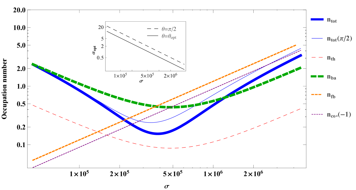
Figure 4: Mechanical steady-state occupancy $n_{\rm{tot}}$ and its individual contributions as functions of the feedback strength $\sigma$, (25), evaluated for the optimized values $\theta_{\rm{opt}}(\sigma),\alpha_{\rm{opt}}(\sigma)$. The parameter set used here is $Q_{\rm{m}}=10^{6},\bar{n}=2.1\times 10^{4}$, which is close to the parameters of [22], and $C_{\rm{q}}=20$. We neglect losses, $\eta=1$. In addition, $n_{\rm{tot}}(\theta=\pi/2)$ is plotted for comparison, where we have evaluated it at the optimal value of $\alpha$ given the suboptimal choice $\theta=\pi/2$, $\alpha_{\rm{opt}}^{(\pi/2)}(\sigma)$. The optimal angle is, for the reasons explained in the main text, approximately constant over the plotted range of $\sigma$, $\theta_{\rm{opt}}(\sigma)\approx 52{}^{\circ}$, and is set by the value of the cooperativity. (Inset) Plot of the functions $\alpha_{\rm{opt}}(\sigma)$ and $\alpha_{\rm{opt}}^{(\pi/2)}(\sigma)$ that minimize $n_{\rm{tot}}$ and $n_{\rm{tot}}(\theta=\pi/2)$, respectively.

Having derived relatively simple expressions for the mechanical steady-state occupancy, we will now plot these functions for optimized parameter values. We assume here that the classical cooperativity $C_{\rm{cl}}$ is fixed (at the maximal value permitted by the given experimental circumstances). For purposes of demonstrating the benefit of varying $\theta$ in the quantum regime of feedback cooling, we consider the limit of large quantum cooperativity,

$$C_{\rm{q}}\equiv C_{\rm{cl}}/\bar{n}\gtrsim 1.$$ (48)

This is the regime where the optical readout rate $\Gamma_{\rm{meas}}$ of the mechanical position exceeds the thermal decoherence rate $\gamma_{\rm{m}}\bar{n}$. We focus here on the limit of ideal detection $\eta=1$.

In Fig. 4 we plot $n_{\rm{tot}}$ and its components, Eqs. (37-42), as a function of the feedback parameter $\sigma$. We do so using the analytically optimized values $\theta_{\rm{opt}}(\sigma)$, Eq. (46), and $\alpha_{\rm{opt}}(\sigma)$ which is found by minimizing Eq. (47), as the roots of higher order polynomials. This gives a sense of how the achievable performance varies as the feedback gain is increased. As expected from the discussion above, the ratio of thermal noise to back action remains constant as $\sigma$ is varied and is solely determined by the quantum cooperativity. For weak feedback $\sigma$ a large cut-off frequency can be afforded (see Fig. 4, inset). Therefore an increase in $\sigma$ leads to further suppression of thermal and back-action noise. However, as $\sigma$ increases beyond its optimal value, the influence of the imprecision noise must be curbed by $\alpha\sim 1$ for which no further suppression of the thermal and back-action noise is possible without paying an even larger penalty from the other sources. This trade-off determines the minimum achievable value of $n_{\rm{tot}}$. We note the following approximate scaling $\alpha_{\rm{opt}}\propto\sigma^{-1}$ from Fig. 4 (inset), which explains, in view of Eq. (47), why the ratio $n_{\rm{fb}}/n_{\rm{co}}$ is seen to be constant in Fig. 4. The scaling also explains, in view of Eq. (46), why the optimal angle is approximately independed on the value of $\sigma$.

Having determined the individual contributions to $n_{\rm{tot}}$ and their behavior in the “graphical minimization” with respect to the feedback strength $\sigma$, we plot the achievable minimum occupancy $n_{\rm{tot}}$ as a function of $C_{\rm{q}}$ in Fig. 5. Subfigures a and b together clearly demonstrate the necessity of adapting the measurement quadrature via $\theta$ in order to get as close to the ground state as possible. For small values of $C_{\rm{q}}\lesssim 1$ we find $\theta_{\rm{opt}}\approx\pi/2$, whereas $\theta_{\rm{opt}}\rightarrow\pi/4$ as $C_{\rm{q}}$ increases, which is consistent with the intuitive discussion in Sec. 4. Note however that $n_{\rm{tot}}(C_{\rm{q}})$ in Fig. 5a exhibits a finite global minimum for both the special case of $\theta=\pi/2$ and using the optimized $\theta=\theta_{\rm{opt}}(C_{\rm{q}})$. For values of $C_{\rm{q}}$ exceeding the minimum point, $\theta_{\rm{opt}}$ drops below $\pi/4$ to compensate for the unnecessarily large (direct) back action. We ascribe the appearance of the minimum in $n_{\rm{tot}}(C_{\rm{q}})$ to our suboptimal choice (21) for the feedback gain function, $\mu(\omega)$. This can be understood in terms of suboptimal mapping of the light quadratures to the mechanical mode as discussed in Sec. 4. Fig. 5c shows the optimal value of the feedback frequency cut-off $\alpha_{\rm{opt}}(C_{\rm{q}})$, which approaches order unity from above as $C_{\rm{q}}$ increases towards the optimum. Similar to the situation in Fig. 4, the decreasing behavior of $\alpha_{\rm{opt}}(C_{\rm{q}})$ reflects the need to suppress the bandwidth of the feedback noise when the feedback gain increases.

From Fig. 5 we conclude that it becomes relevant to choose a homodyne quadrature angle $\theta\neq\pi/2$ in the regime of very large quantum cooperativty, $C_{\rm q}\gg 1$. While the reduction in $n_{\rm tot}$ gained in this way will be small in absolute numbers, it can be significant relative to the value of $n_{\rm tot}$ achieved with $\theta=\pi/2$.

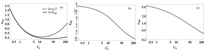
Figure 5: Optimized cooling for the same parameters as in Fig. 4, but with $C_{\rm{q}}$ as an independent variable. (a) $n_{\rm{tot}}$ as a function of $C_{\rm{q}}$ evaluated at the optimal values $\theta_{\rm{opt}}(C_{\rm{q}}),\alpha_{\rm{opt}}(C_{\rm{q}}),\sigma(C_{\rm{q}})$. For comparison, we also plot the curve resulting from the suboptimal choice $\theta=\pi/2$ evaluating at optimal parameter values given this choice, $\alpha_{\rm{opt}}^{(\pi/2)}(C_{\rm{q}}),\sigma^{(\pi/2)}(C_{\rm{q}})$. Both functions have a local minimum, which can likely be ascribed to the suboptimal functional form of the feedback gain $\mu(\omega)$ considered throughout this analysis. (b, c) Optimal quadrature angle $\theta_{\rm{opt}}(C_{\rm{q}})$ and feedback cut-off parameter $\alpha_{\rm{opt}}(C_{\rm{q}})$.

7 Conclusion and outlook

Simultaneous optimization of the feedback gain $\mu(\omega)$ and the homodyne quadrature angle $\theta$ are crucial elements of realizing the full potential of feedback cooling in the quantum regime.

As an outlook, we will point out two intriguing theoretical challenges on the subject of feedback cooling in the quantum regime. The analysis and optimization presented here was based on a particular choice for the feedback filter function $\mu(\omega)$, as stated in Eq. (21), implementing a derivative-type feedback combined with a low-pass filter. While this choice of $\mu(\omega)$ has desirable features for purposes of cooling there is no reason to believe that the form of $\mu(\omega)$ assumed here is optimal from a theoretical perspective. Hence, this work does not establish the ultimate limit of performance for the scheme. This is an open question within quantum control theory (to the knowledge of the authors) and merits further investigation. The authors of Ref. [22] made progress in this direction by deriving the optimal filter minimizing the position fluctuations for feedback based on measurements of the phase quadrature. As the authors emphasize, this filter includes spectrally sharp features, which will require very fast electronics to implement and may not be feasible in practice. Accordingly, the employed feedback filter was a delay line combined with a low-pass filter [22, 23]. This choice is simpler to implement in practice, but is in fact mathematically more cumbersome to treat than the form of $\mu(\omega)$ assumed here.

Another important remark should be made on the generality of the analysis presented here. As mentioned in Sec. 2, we adopted here a prescription for including feedback in the Heisenberg-Langevin equations as done in several previous studies found in the literature. While this approach can be justified rigorously for Markovian feedback, no such derivation is available for Non-Markovian feedback. Rigorous descriptions of Non-Markovian feedback exist based on the stochastic Schrödinger equation, cf. [29, 34]. However, it appears that a derivation of the corresponding Heisenberg-Langevin description has not been reported in the literature so far. It is therefore possible that this and previous studies neglect corrections due to the non-commutativity of Heisenberg operators at unequal times which may become significant in the quantum regime of operation. Only when these theoretical challenges have been addressed, the ultimate quantum limits of feedback cooling can be established.

8 References

Appendix A Stability condition

In this Appendix we derive the stability condition for the optomechanical system subject to feedback. The validity of the linearized equations of motion given in the main text hinges on the fulfillment of this condition. Stability is ensured if the real part of all poles of the effective mechanical susceptibility $\chi_{\rm{eff}}(\omega)$ are negative. The character of the poles can be determined using the Routh-Hurwitz criterion [33], which in the present case leads to a single non-trivial stability condition,

$$1 + \sigma+\frac{1}{\alpha^{2}}+\frac{1}{Q_{\rm{m}}\alpha}+\frac{\sigma}{Q_{\rm{m}}\alpha}$$

$$+ \beta^{3}\biggl{\{}\frac{1}{Q_{\rm{m}}}+\frac{1}{\alpha}+\alpha\biggr{\}}$$

$$+ \beta^{2}\biggl{\{}1+\frac{1}{Q_{\rm{m}}^{2}}+\frac{1}{\alpha^{2}}+\frac{2}{Q_{\rm{m}}\alpha}+\frac{\alpha}{Q_{\rm{m}}}$$

$$+ \frac{\sigma}{Q_{\rm{m}}}\left(\frac{1}{Q_{\rm{m}}}+\frac{1}{\alpha}+\alpha\right)\biggr{\}}$$

$$+ \beta\biggl{\{}\alpha+\alpha\sigma+\frac{2}{Q_{\rm{m}}}+\frac{1}{Q_{\rm{m}}\alpha^{2}}+\frac{1}{\alpha}+\frac{1}{Q_{\rm{m}}^{2}\alpha}$$

$$+ \frac{\sigma}{Q_{\rm{m}}}\left(1+\frac{1}{Q_{\rm{m}}\alpha}\right)\biggr{\}}$$

$$- \left(\sigma\beta^{2}+\frac{\beta\sigma}{\alpha}+\frac{\beta\sigma^{2}\alpha}{Q_{\rm{m}}}\right)>0,$$

where we have introduced the optomechanical sideband resolution factor $\beta\equiv 2\omega_{\rm{m}}/\kappa$, the mechanical quality factor $Q_{\rm{m}}\equiv\omega_{\rm{m}}/\gamma_{\rm{m}}$, and (as in the main text) the rescaled dimensionless feedback gain is $\sigma\equiv 2\mu_{\rm{fb}}g_{\rm{om}}\omega_{\rm{m}}/\kappa\gamma_{\rm{m}}$. The feedback gain only enters the stability criterion (A) via the rescaled definition $\sigma$, which is why no explicit dependence on the measurement quadrature angle $\theta$ enters. (If desired, Eq. (A) can be restated in terms of $\theta$ and the absolute gain $\tilde{\sigma}$ as pointed out in the main text below Eq. (25).) Note that in the main text we primarily focus on the idealized bad-cavity limit, $\kappa\rightarrow\infty$, in which the stability criterion A is trivially fulfilled.

Appendix B Mechanical steady-state occupation $n_{\rm{tot}}$ for arbitrary $\kappa$

In the main text we focus on the idealized bad-cavity limit, $\kappa\rightarrow\infty$, for simplicity of analysis. Here we will give the exact expression for the mechanical steady-state occupation number, $n_{\rm{tot}}$, valid for arbitrary values of $\kappa$ (insofar as the stability criterion of A is fulfilled). Retracing the steps taken in Sec. 5 of the main text, we decompose the mechanical occupancy into contributions according to physical origin

$$n_{\rm{tot}}=\frac{n_{X}+n_{P}}{2}-\frac{1}{2}=n_{\rm{th}}+n_{\rm{ba}}+n_{\rm{fb}}+n_{\rm{co}}+n_{v}-\frac{1}{2},$$ (50)

where $n_{X}$ and $n_{P}$ are the contributions from the position and momentum variances, respectively. As will be clear from the expressions below, the steady state of the mechanical mode in the presence of feedback generally does not obey equipartition of energy, i.e., we will have $n_{X}\neq n_{P}$. To display the position and momentum contributions separately, we will decompose the various noise contributions as $n_{i}=(n_{i,X}+n_{i,P})/2$ below. These will be expressed in terms of the following dimensionless parameters: The classical optomechanical cooperativity $C_{\rm{cl}}=4g_{\rm{om}}^{2}/\kappa\gamma_{\rm{m}}$, the rescaled feedback gain $\sigma=2\mu_{\rm{fb}}g_{\rm{om}}\omega_{\rm{m}}/\kappa\gamma_{\rm{m}}$, the optomechanical sideband resolution parameter $\beta=2\omega_{\rm{m}}/\kappa$, the mechanical quality factor $Q_{\rm{m}}=\omega_{\rm{m}}/\gamma_{\rm{m}}$, and the feedback frequency cut-off parameter $\alpha\equiv\omega_{\rm{fb}}/\omega_{\rm{m}}$. All expressions below are organized according to the parameters $\beta$ and $1/Q_{\rm{m}}$, which are small in the typical parameter regime of interest.

The exact value of the mechanical steady-state occupancy $n_{\rm{tot}}$, valid for all stable values of $\kappa$, is given by the following contributions in Eq. (50): The thermal heating from intrinsic mechanical damping,

$$n_{\rm{th}}=\frac{n_{\rm{th},X}+n_{\rm{th},P}}{2}$$ (51)

$$n_{\rm{th},X} = \frac{1}{S_{\rm{m}}}\left(\bar{n}+\frac{1}{2}\right)\Bigg{[}1+\frac{1}{\alpha^{2}}+\frac{1}{\alpha Q_{\rm{m}}}$$

$$+ \beta\left\{\frac{1}{\alpha}+\alpha+\frac{1}{Q_{\rm{m}}}\left(2+\frac{1}{\alpha^{2}}-\sigma\right)+\frac{1}{\alpha Q_{\rm{m}}^{2}}\right\}$$

$$+ \beta^{2}\left\{1+\frac{1}{\alpha^{2}}+\frac{1}{Q_{\rm{m}}}\left(\frac{2}{\alpha}+\alpha+\frac{\sigma}{\alpha}\right)+\frac{1}{Q_{\rm{m}}^{2}}\right\}$$

$$+ \beta^{3}\left\{1+\frac{1}{\alpha^{2}}+\frac{1}{Q_{\rm{m}}}\right\}\Bigg{]}$$

$$n_{\rm{th},P} = \frac{1}{S_{\rm{m}}}\left(\bar{n}+\frac{1}{2}\right)\Bigg{[}1+\frac{1}{\alpha^{2}}+\frac{1}{\alpha Q_{m}}\left(1+\sigma\right)$$

$$+ \beta\left\{\frac{1}{\alpha}+\alpha+\frac{1}{Q_{\rm{m}}}\left(2+\frac{1}{\alpha^{2}}+\sigma\right)+\frac{1+\sigma}{\alpha Q_{\rm{m}}^{2}}\right\}$$

$$+ \beta^{2}\biggl{\{}1+\frac{1}{\alpha^{2}}+\frac{1}{Q_{\rm{m}}}\left(\frac{2}{\alpha}+\alpha+\frac{\sigma}{\alpha}+\alpha\sigma\right)$$

$$+ \frac{1+\sigma}{Q_{\rm{m}}^{2}}\biggr{\}}$$

$$+ \beta^{3}\left\{1+\frac{1}{\alpha^{2}}+\frac{1}{Q_{\rm{m}}}\right\}\Bigg{]},$$

the direct back-action heating,

$$n_{\rm{ba}}=\frac{n_{\rm{ba},X}+n_{\rm{ba},P}}{2}$$ (54)

$$n_{\rm{ba},X} = \frac{1}{S_{\rm{m}}}\frac{C_{\rm{cl}}}{4}\Bigg{[}1+\frac{1}{\alpha^{2}}+\frac{1}{\alpha Q_{\rm{m}}}$$

$$+ \beta\left\{\frac{1}{\alpha}+\alpha+\frac{1}{Q_{\rm{m}}}\left(2+\frac{1}{\alpha^{2}}-\sigma\right)+\frac{1}{\alpha Q_{\rm{m}}^{2}}\right\}$$

$$+ \beta^{2}\left\{\frac{1}{Q_{\rm{m}}}\left(\frac{1}{\alpha}+\alpha\right)+\frac{1}{Q_{\rm{m}}^{2}}\right\}\}$$

$$n_{\rm{ba},P} = \frac{1}{S_{\rm{m}}}\frac{C_{\rm{cl}}}{4}\Bigg{[}1+\frac{1}{\alpha^{2}}+\frac{1}{\alpha Q_{\rm{m}}}\left(1+\sigma\right)$$

$$+ \beta\left\{\frac{1}{\alpha}+\alpha+\frac{1}{Q_{\rm{m}}}\right\}\Bigg{]},$$

the imprecision noise heating,

$$n_{\rm{fb}}=\frac{n_{\rm{fb},X}+n_{\rm{fb},P}}{2}$$ (57)

$$n_{\rm{fb},X} =\frac{1}{S_{\rm{m}}}\frac{\sigma^{2}}{2C_{\rm{cl}}}\Bigg{[}1+\beta\left\{\alpha+\frac{1}{Q_{\rm{m}}}\right\}$$

$$+\beta^{2}\left\{1+\frac{\alpha}{Q_{\rm{m}}}\left(1+\sigma\right)\right\}+\beta^{3}\alpha\Bigg{]}\csc^{2}(\theta),$$

$$n_{\rm{fb},P} =\frac{1}{S_{\rm{m}}}\frac{\sigma^{2}}{2C_{\rm{cl}}}\Bigg{[}1+\frac{\alpha}{Q_{\rm{m}}}\left(1+\sigma\right)$$

$$+\beta\left\{\alpha+\frac{1}{Q_{\rm{m}}}\left(1+\alpha^{2}+\alpha^{2}\sigma\right)+\frac{\alpha}{Q_{\rm{m}}^{2}}\left(1+\sigma\right)\right\}$$

$$+\beta^{2}\left\{1+\frac{\alpha}{Q_{\rm{m}}}\left(2+\sigma\right)+\frac{\alpha^{2}}{Q_{\rm{m}}^{2}}\left(1+\sigma\right)\right\}$$

$$+\beta^{3}\left\{\alpha+\frac{\alpha^{2}}{Q_{\rm{m}}}\right\}\Bigg{]}\csc^{2}(\theta).$$

the correction term due to correlations between the direct back-action and the measurement imprecision fluctuations ($n_{\rm{co}}<0$ for parameter choices of interest)

$$n_{\rm{co}}=\frac{n_{\rm{co},X}+n_{\rm{co},P}}{2}$$ (60)

$$n_{\rm{co},X} =-\frac{1}{S_{\rm{m}}}\frac{\sigma}{4\alpha}\Biggl{[}1+\beta\left\{2\alpha+\frac{1}{Q_{\rm{m}}}\right\}$$

$$+\beta^{2}\left\{\alpha^{2}+\frac{\alpha}{Q_{\rm{m}}}\right\}\Biggr{]}\cot(\theta),$$

$$n_{\rm{co},P} =-\frac{1}{S_{\rm{m}}}\frac{\sigma}{4\alpha}\Biggl{[}1+\frac{\alpha}{Q_{\rm{m}}}\left(1+\sigma\right)$$

$$+\beta\left\{2\alpha+\frac{\alpha^{2}}{Q_{\rm{m}}}\left(1+\sigma\right)\right\}+\beta^{2}\alpha^{2}\Biggr{]}\cot(\theta),$$

and finally the excess imprecision noise due to optical losses and imperfect detection ($\eta<1$)

$$n_{v}=n_{\rm{fb}}\left(\eta^{-1}-1\right),$$ (63)

where the denominator of these expressions is

$$S_{\rm{m}} =1+\sigma+\frac{1}{\alpha^{2}}+\frac{1}{\alpha\rm{Q}_{\rm{m}}}(1+\sigma)$$

$$+\beta\biggl{\{}\frac{1}{\alpha}\left(1-\sigma\right)+\left(\alpha+\frac{1}{\alpha\rm{Q}_{\rm{m}}^{2}}\right)(1+\sigma)$$

$$+\frac{1}{\rm{Q}_{\rm{m}}}\left(2+\frac{1}{\alpha^{2}}+\sigma-\sigma^{2}\right)\biggr{\}}$$

$$+\beta^{2}\biggl{\{}1+\frac{1}{\alpha^{2}}-\sigma+\frac{1}{Q_{\rm{m}}}\left(\frac{1}{Q_{\rm{m}}}+\alpha\right)\left(1+\sigma\right)$$

$$+\frac{1}{\alpha Q_{\rm{m}}}\left(2+\sigma\right)\biggr{\}}$$

$$+\beta^{3}\left\{\frac{1}{\alpha}+\alpha+\frac{1}{Q_{\rm{m}}}\right\}.$$

These formulas generalize the expressions given in Ref. [21] in which the special case $\theta=\pi/2$ was considered.

Appendix C Integrals over rational functions

We consider integrals over rational functions of the form

$$\int_{-\infty}^{\infty}\frac{g_{n}\left(\omega\right)}{h_{n}\left(\omega\right)h_{n}\left(-\omega\right)}d\omega,$$

where $g_{n}$ and $h_{n}$ are polynomials of the following form

$$g_{n}\left(\omega\right)=b_{0}\omega^{2n-2}+b_{1}\omega^{2n-4}+\cdots+b_{n-2}\omega^{2}+b_{n-1}$$ (65)

$$h_{n}\left(\omega\right)=a_{0}\omega^{n}+a_{1}\omega^{n-1}+\cdots+a_{n-1}\omega+a_{n}$$ (66)

and we assume that $a_{0}\neq 0$ and that all the roots of $h_{n}\left(\omega\right)$ lie in the upper half plane. The solution to the integral can be stated in terms of the determinants of two square matrices $\Delta_{n},M_{n}$ of dimension $n$. Setting $a_{k}=0$ for any $k\notin\{0,\ldots,n\}$ the $(i,j)^{\prime}\rm{th}$ entries of the matrices can be stated as

$$(\Delta_{n})_{i,j} = a_{2j-i}$$ (67)

$$(M_{n})_{i,j} = \delta_{1,i}b_{j-1}+(1-\delta_{1,i})a_{2j-i},$$ (68)

where $\delta_{i,j}$ is the Kronecker delta function. The matrices differ only by their first rows as is clear from their explicit form,

$$\Delta_{n}=\left(\begin{array}[]{ccccc}a_{1}&a_{3}&a_{5}&\ldots&0\\ a_{0}&a_{2}&a_{4}&&0\\ 0&a_{1}&a_{3}&&0\\ \vdots&&&\ddots&\\ 0&0&0&&a_{n}\end{array}\right),\,\,\,$$ (69)

$$M_{n}=\left(\begin{array}[]{ccccc}b_{0}&b_{1}&b_{2}&\ldots&b_{n-1}\\ a_{0}&a_{2}&a_{4}&&0\\ 0&a_{1}&a_{3}&&0\\ \vdots&&&\ddots&\\ 0&0&0&&a_{n}\end{array}\right).$$ (70)

The value of the integral can now be stated as

$$\int_{-\infty}^{\infty}\frac{g_{n}\left(\omega\right)}{h_{n}\left(\omega\right)h_{n}\left(-\omega\right)}d\omega=i(-1)^{n+1}\frac{\pi}{a_{0}}\frac{\det M_{n}}{\det\Delta_{n}}.$$ (71)

This formula was used to evaluate $n_{\rm{tot}}$ in terms of integrals over spectral densities as presented in the main text. The formula (71) appears in Ref. [35] on Page 253, however, there the factor $(-1)^{n+1}$ was omitted.

References

- [1] Stefan L. Danilishin and Farid Ya. Khalili. Quantum measurement theory in gravitational-wave detectors. Living Reviews in Relativity, 15, 2012.
- [2] Yanbei Chen. Macroscopic quantum mechanics: theory and experimental concepts of optomechanics. Journal of Physics B: Atomic, Molecular and Optical Physics, 46(10):104001, may 2013.
- [3] M. Aspelmeyer, S. Gröblacher, K. Hammerer, and N. Kiesel. Quantum optomechanics—throwing a glance [invited]. J. Opt. Soc. Am. B, 27(6):A189–A197, Jun 2010.
- [4] Markus Aspelmeyer, Tobias J. Kippenberg, and Florian Marquardt. Cavity optomechanics. Rev. Mod. Phys., 86:1391–1452, Dec 2014.
- [5] A D O’Connell, M Hofheinz, M Ansmann, Radoslaw C Bialczak, M Lenander, Erik Lucero, M Neeley, D Sank, H Wang, M Weides, J Wenner, John M Martinis, and A N Cleland. Quantum ground state and single-phonon control of a mechanical resonator. Nature, 464(7289):697–703, apr 2010.
- [6] T. A. Palomaki, J. W. Harlow, J. D. Teufel, R. W. Simmonds, and K. W. Lehnert. Coherent state transfer between itinerant microwave fields and a mechanical oscillator. Nature, 495(7440):210–214, 03 2013.
- [7] Joerg Bochmann, Amit Vainsencher, David D. Awschalom, and Andrew N. Cleland. Nanomechanical coupling between microwave and optical photons. Nat Phys, 9(11):712–716, 11 2013.
- [8] T. Bagci, A. Simonsen, S. Schmid, L. G. Villanueva, E. Zeuthen, J. Appel, J. M. Taylor, A. Sørensen, K. Usami, A. Schliesser, and E. S. Polzik. Optical detection of radio waves through a nanomechanical transducer. Nature, 507(7490):81–85, 03 2014.
- [9] R. W. Andrews, R. W. Peterson, T. P. Purdy, K. Cicak, R. W. Simmonds, C. A. Regal, and K. W. Lehnert. Bidirectional and efficient conversion between microwave and optical light. Nat Phys, 10(4):321–326, 04 2014.
- [10] Mahdi Hosseini, Giovanni Guccione, Harry J. Slatyer, Ben C. Buchler, and Ping Koy Lam. Multimode laser cooling and ultra-high sensitivity force sensing with nanowires. Nat Commun, 5:–, August 2014.
- [11] T. Rocheleau, T. Ndukum, C. Macklin, J. B. Hertzberg, A. A. Clerk, and K. C. Schwab. Preparation and detection of a mechanical resonator near the ground state of motion. Nature, 463(7277):72–75, 01 2010.
- [12] J. D. Teufel, T. Donner, Dale Li, J. W. Harlow, M. S. Allman, K. Cicak, A. J. Sirois, J. D. Whittaker, K. W. Lehnert, and R. W. Simmonds. Sideband cooling of micromechanical motion to the quantum ground state. Nature, 475(7356):359–363, 07 2011.
- [13] Jasper Chan, T. P. Mayer Alegre, Amir H. Safavi-Naeini, Jeff T. Hill, Alex Krause, Simon Groblacher, Markus Aspelmeyer, and Oskar Painter. Laser cooling of a nanomechanical oscillator into its quantum ground state. Nature, 478(7367):89–92, 10 2011.
- [14] E. Verhagen, S. Deleglise, S. Weis, A. Schliesser, and T. J. Kippenberg. Quantum-coherent coupling of a mechanical oscillator to an optical cavity mode. Nature, 482(7383):63–67, 02 2012.
- [15] Daniel W C Brooks, Thierry Botter, Sydney Schreppler, Thomas P Purdy, Nathan Brahms, and Dan M Stamper-Kurn. Non-classical light generated by quantum-noise-driven cavity optomechanics. Nature, 488(7412):476–80, aug 2012.
- [16] Amir H. Safavi-Naeini, Simon Groeblacher, Jeff T. Hill, Jasper Chan, Markus Aspelmeyer, and Oskar Painter. Squeezing of light via reflection from a silicon micromechanical resonator. Nature, page 24, feb 2013.
- [17] T. P. Purdy, P.-L. Yu, R. W. Peterson, N. S. Kampel, and C. A. Regal. Strong optomechanical squeezing of light. Phys. Rev. X, 3:031012, Sep 2013.
- [18] Ralf Riedinger, Sungkun Hong, Richard A. Norte, Joshua A. Slater, Juying Shang, Alexander G. Krause, Vikas Anant, Markus Aspelmeyer, and Simon Gröblacher. Non-classical correlations between single photons and phonons from a mechanical oscillator. Nature, 530(7590):313–316, February 2016.
- [19] E. E. Wollman, C. U. Lei, A. J. Weinstein, J. Suh, A. Kronwald, F. Marquardt, A. A. Clerk, and K. C. Schwab. Quantum squeezing of motion in a mechanical resonator. Science, 349(6251):952–955, 2015.
- [20] T A Palomaki, J D Teufel, R W Simmonds, and K W Lehnert. Entangling mechanical motion with microwave fields. Science (New York, N.Y.), 342(6159):710–3, nov 2013.
- [21] C. Genes, D. Vitali, P. Tombesi, S. Gigan, and M. Aspelmeyer. Ground-state cooling of a micromechanical oscillator: Comparing cold damping and cavity-assisted cooling schemes. Phys. Rev. A, 77:033804, Mar 2008.
- [22] D. J. Wilson, V. Sudhir, N. Piro, R. Schilling, A. Ghadimi, and T. J. Kippenberg. Measurement-based control of a mechanical oscillator at its thermal decoherence rate. Nature, 524(7565):325–329, August 2015.
- [23] V. Sudhir, D. J. Wilson, R. Schilling, H. Schütz, A. Ghadimi, A. Nunnenkamp, and T. J. Kippenberg. Appearance and disappearance of quantum correlations in measurement-based feedback control of a mechanical oscillator. ArXiv e-prints, February 2016.
- [24] Paul Busch, Pekka Lahti, and Reinhard F. Werner. Colloquium : Quantum root-mean-square error and measurement uncertainty relations. Rev. Mod. Phys., 86:1261–1281, Dec 2014.
- [25] S. P. Vyatchanin and A. B. Matsko. Quantum limit on force measurements. Journal of Experimental and Theoretical Physics, 77(2):218, 1993.
- [26] H. J. Kimble, Yuri Levin, Andrey B. Matsko, Kip S. Thorne, and Sergey P. Vyatchanin. Conversion of conventional gravitational-wave interferometers into quantum nondemolition interferometers by modifying their input and/or output optics. Phys. Rev. D, 65:022002, Dec 2001.
- [27] C. Genes, A. Mari, D. Vitali, and P. Tombesi. Chapter 2 quantum effects in optomechanical systems. In Advances in Atomic Molecular and Optical Physics, volume 57 of Advances In Atomic, Molecular, and Optical Physics, pages 33 – 86. Academic Press, 2009.
- [28] Sebastian G. Hofer and Klemens Hammerer. Entanglement-enhanced time-continuous quantum control in optomechanics. Phys. Rev. A, 91:033822, Mar 2015.
- [29] H. M. Wiseman. Quantum theory of continuous feedback. Phys. Rev. A, 49:2133–2150, Mar 1994.
- [30] Kurt Jacobs. Quantum Measurement Theory and its Applications. Cambridge University Press, 2014.
- [31] Stefano Mancini, David Vitali, and Paolo Tombesi. Optomechanical cooling of a macroscopic oscillator by homodyne feedback. Phys. Rev. Lett., 80:688–691, Jan 1998.
- [32] Vittorio Giovannetti and David Vitali. Phase-noise measurement in a cavity with a movable mirror undergoing quantum brownian motion. Phys. Rev. A, 63:023812, Jan 2001.
- [33] E. X. Dejesus and C. Kaufman. Routh-Hurwitz criterion in the examination of eigenvalues of a system of nonlinear ordinary differential equations. Phys. Rev. Lett., 35:5288–5290, June 1987.
- [34] V. Giovannetti, P. Tombesi, and D. Vitali. Non-markovian quantum feedback from homodyne measurements: The effect of a nonzero feedback delay time. Phys. Rev. A, 60:1549–1561, Aug 1999.
- [35] I. S. Gradshteyn and I. M. Ryzhik (Seventh Edition). 3.-4 - definite integrals of elementary functions. In Table of Integrals, Series, and Products (Corrected and Enlarged Edition), pages 211 – 625. Academic Press, corrected and enlarged edition edition, 1980.