Mastering $2048$ with Delayed Temporal Coherence Learning, Multi-Stage Weight Promotion, Redundant Encoding
and Carousel Shaping

Abstract

$2048$ is an engaging single-player nondeterministic video puzzle game, which, thanks to the simple rules and hard-to-master gameplay, has gained massive popularity in recent years. As $2048$ can be conveniently embedded into the discrete-state Markov decision processes framework, we treat it as a testbed for evaluating existing and new methods in reinforcement learning. With the aim to develop a strong $2048$ playing program, we employ temporal difference learning with systematic $n$-tuple networks. We show that this basic method can be significantly improved with temporal coherence learning, multi-stage function approximator with weight promotion, carousel shaping, and redundant encoding. In addition, we demonstrate how to take advantage of the characteristics of the $n$-tuple network, to improve the algorithmic effectiveness of the learning process by delaying the (decayed) update and applying lock-free optimistic parallelism to effortlessly make advantage of multiple CPU cores. This way, we were able to develop the best known $2048$ playing program to date, which confirms the effectiveness of the introduced methods for discrete-state Markov decision problems.

I Introduction

$2048$ is an engaging single-player nondeterministic puzzle game which has gained massive popularity in recent years. Already in the first week after its release, in March 2014, more than $500$ man-years had been spent playing the game, according to its author. Some of the numerous $2048$ clones were downloaded tens of millions of times from the online mobile app stores, making it a part of global culture.

Since the human experience with the game says that it is not trivial to master, this raises the natural question how well a computer program can handle it?

From the perspective of artificial intelligence, the simple rules and hard-to-master complexity in the presence of non-determinism makes $2048$ an ideal benchmark for learning and planning algorithms. As $2048$ can be conveniently described in terms of Markov decision process (MDP), in this paper, we treat $2048$ as a challenging testbed to evaluate the effectiveness of some existing and novel ideas in reinforcement learning for discrete-state MDPs [8].

For this purpose, we build upon our earlier work [31], in which we demonstrated a temporal difference (TD) learning-based approach to $2048$. The algorithm used the standard TD($0$) rule [30] to learn the weights of an $n$-tuple network [15] approximating the afterstate-value function. In this paper, we extend this method in several directions. First, we show the effectiveness of temporal coherence learning [3], a technique for automatically tuning the learning rates. Second, we introduce three novel methods that concern both the learning process and the value function approximator: i) multi-stage weight promotion, ii) carousel shaping, and iii) redundant encoding, which are the primary contributions of this paper. The computational experiments reveal that the effectiveness of the first two techniques depend on the depth of the tree the controller is allowed to search. The synergy of the above-mentioned techniques allowed us to obtain the best $2048$ controller to date.

This result would not be possible without paying attention to the computational effectiveness of the learning process. In this line, we also introduce delayed temporal difference (delayed-TD($\lambda$)), an online learning algorithm based on TD($\lambda$) whose performance, when used with $n$-tuple network function approximator, is vastly independent of the decay parameter $\lambda$. Finally, we demonstrate that for large lookup table-based approximators such as $n$-tuple networks, we can make use of multithreading capabilities of modern CPUs by imposing the lock-free optimistic parallelism on the learning process.

This work confirms the virtues of $n$-tuples network as the function approximators. The results for $2048$ indicate that they are effective and efficient even when involving a billion parameters, which has never been shown before.

Although the methods introduced in this paper were developed for $2048$, they are general, thus can be transferred to any discrete-state Markov decision problems, classical board games included. The methodology as a whole can be directly used to solve similar, small-board, nondeterministic puzzle games such as $1024$, Threes, or numerous $2048$ clones.

II The Game of 2048

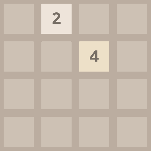
(a) A sample initial game state. All four actions are available.

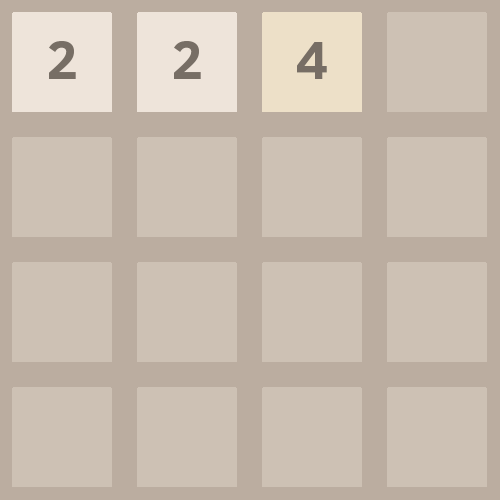
(b) After making the up action, a $2$-tile appeared in the upper left corner.

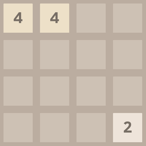
(c) The left action in $s_{1}$ was rewared by $4$ for merging two $2$-tiles.

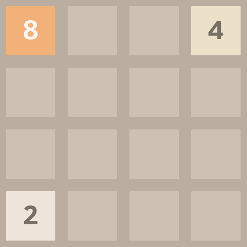
(d) The left action was rewarded by $8$ for merging two $4$-tiles.

Fig 1: A sample sequence of initial states and actions.

$2048$ is a single-player, nondeterministic, perfect information video game played on a $4\times 4$ board. Each square of the board can either be empty or contain a single $v$-tile, where $v$ is a positive power of two and denotes the value of a tile. The game starts with two randomly generated tiles. Each time a random tile is to be generated, a $2$-tile (with probability $p_{2}=0.9$) or a $4$-tile ($p_{4}=0.1$) is placed on an empty square of the board. A sample initial state is shown in Fig. 1a.

The objective of the game is to slide the tiles and merge the adjacent ones to ultimately create a tile with the value of $2048$. At each turn the player makes a move consisting in sliding all the tiles in one of the four directions: up, right, down or left. A move is legal if at least one tile is slid. After each move, a new $2$-tile or $4$-tile is randomly generated according to the aforementioned probabilities. For instance, Fig. 1b illustrates that after sliding up both initial tiles, a random $2$-tile is placed in the upper left corner.

A key operation that allows obtaining tiles of larger values consists in merging adjacent tiles. When making a move, each pair of adjacent tiles of the same value is combined into a single tile along the move direction. The new tile is assigned the total value of the two joined tiles. Additionally, the player gains a reward equal to the value of the new tile for each such merge. Figure 1c shows the board resulting from combining two $2$-tiles in the upper row when sliding the tiles in the left direction. Another left move leads to creating an $8$-tile (see Fig. 1d). The moves generate rewards of $4$ and $8$, respectively.

The game is considered won when a $2048$-tile appears on the board. However, players can continue the game even after reaching this tile. The game terminates when no legal moves are possible, i.e., all squares are occupied, and no two adjacent tiles are sharing the same value. The game score is the sum of rewards obtained throughout the game.

III Related Work

$2048$ was first approached by Szubert and Jaśkowski [31] who employed $\text{TD}(0)$ with $1$ million training episodes to learn an afterstate-value function represented by a systematic $n$-tuple network [11]. Their best function involved nearly $23$ million parameters and scored $100\,178$ on average at $1$-ply. Wu et al. [38] has later extended this work by employing TD($0$) with $5$ million training games to learn a larger systematic $n$-tuple system with $67$ million parameters, scoring $142\,727$ on average. By employing three such $n$-tuple networks enabled at different stages of the game along with expectimax with depth $5$, they were able to achieve $328\,946$ points on average. Further refinement its controller lead to scoring $443\,526$ on average [40]. Recently, Oka and Matsuzaki systematically evaluated a different n-tuple shapes to construct a $1$-ply controller achieving $234\,136$ points on average [21]. Rodgers and Levine investigated the use of various tree search techniques for $2048$, but were only able to score $140\,000$ on average [22]. There are also numerous $2048$ open source controllers available on the Internet. To the best of our knowledge, the most successful of them is by Xiao et al [39]. It is based on an efficient bitboard representation with a variable-depth expectimax, transposition tables and a hand-designed state-evaluation heuristic, which has been optimized by CMA-ES [10]. Their player average score is $442\,419$.

Mehta proved that the $n\times n$ version of the game $2048$ is PSPACE hard [18] assuming that the random moves are known in advance. The game has also been recently appreciated as a tool for teaching computer science and artificial intelligence techniques [20].

The roots of reinforcement learning [14] in games can be tracked down to Samuel’s famous work on Checkers [25], but it was not popularized until the Tesauro’s TD-Gammon, a master-level program for Backgammon [34] obtained by temporal difference learning. Various reinforcement learning algorithms were applied with success to other games such as Othello [6, 15, 32], Connect 4 [37], Tetris [27, 13], or Atari video games [4]. Recently, AlphaGo used reinforcement learning among others to determine weights for a deep artificial neural network to beat a professional Go player [28].

The $n$-tuple network is due to Bledsoe and Browning [5] for optical character recognition. In the context of board games, this idea was popularized by Lucas with its application to Othello [15]. It is, however, worth noticing that a similar concept, called tabular value function, was already used by Buro in his strong Othello-playing Logistello program [6]. From the perspective of reinforcement learning literature, an $n$-tuple network is a variant of tile coding [30], which is another name for Albus’s cerebellar model articulator controller (CMAC) [1].

IV Temporal Difference Learning with N-Tuple Networks

In this section, we introduce all basic concepts for temporal difference learning using $n$-tuple network. The learning framework presented in the last subsection corresponds to the method we used in the previous work [31] for $2048$, and will be the foundation for improvements in the subsequent sections.

IV-A Markov Decision Processes

The game of $2048$ can be conveniently framed as a fully observable, non-discounted discrete Markov Decision Process (MDP). An MDP consists of:

• a set of states $S$,

• a set of actions available in each state $A(s)$, $s\in S$,

• a transition function $T(s^{\prime\prime},s,a)$, which defines the probability of achieving state $s^{\prime\prime}$ when making action $a$ in state $s$, and

• a reward function $R(s)$ defining a reward received as a result of a transition to state $s$.

An agent making decisions in MDP environment follows a policy $\pi:S\rightarrow A$, which defines its behavior in all states. The value or utility of a policy $\pi$ when starting the process from a given state $s\in S$ is the expected sum of rewards:

$$V^{\pi}(s)=\mathbb{E}_{\pi}\left[\sum_{t=0}^{\infty}R(S_{t})|S_{0}=s\right],$$ (1)

where $S_{t}$ is a random variable indicating the state of the process in time $t$ and $\mathbb{E}_{\pi}$ denotes the expected value given that the agent follows policy $\pi$.

The goal is to find the optimal policy $\pi^{*}$ such that for all $s\in S$

$$\pi^{*}(s)=\mathrm{argmax}_{\pi}V^{\pi}(s).$$

As $V^{\pi^{*}}(s)$ is the value of the optimal policy $\pi^{*}$ when following it from state $s$, it can be interpreted as a value of state $s$, and conveniently denoted as $V(s)$.

To solve an MDP, one can directly search the space of policies. Another possibility is to estimate the optimal state-value function $V:S\rightarrow\mathbb{R}$. Then, the optimal policy is a greedy policy w.r.t $V$:

$$\pi^{*}(s)=\mathrm{argmax}_{a\in A(s)}\sum_{s^{\prime\prime}\in S}T(s^{\prime\prime},s,a)V(s^{\prime\prime}).$$ (2)

IV-B Function Approximation

For most practical problems, it is infeasible to represent a value function as a lookup table, with one entry $V(s)$ for each state $s\in S$, since the state space $S$ is too large. For example, the game of 2048 has $(4\times 4)^{18}\approx 4.7\times 10^{21}$ states, which significantly exceeds the memory capabilities of the current computers. This is why, in practice, instead of lookup tables, function approximators are used. A function approximator is a function of a form $V_{\theta}:S\rightarrow\mathbb{R}$, where $\theta$ is a vector of parameters that undergo optimization or learning.

By using a function approximator, the dimensionality of the search space is reduced from $|S|$ to $|\theta|$. As a result, the function approximator gets capabilities to generalize. Thus, the choice of a function approximator is as important as the choice of the learning algorithm itself.

IV-B1 $n$-Tuple Network

One particular type of function approximator is n-tuple network [15], which has been recently successfully applied to board games such as Othello [7, 17, 33, 12], Connect 4 [37], or Tetris [13].

An $n$-tuple network consists of $m$ $n_{i}$-tuples, where $n_{i}$ is tuple’s size. For a given board state $s$, it calculates the sum of values returned by the individual $n$-tuples. The $i$th $n_{i}$-tuple, for $i=1\dots m$, consists of a predetermined sequence of board locations $(loc_{ij})_{j=1\dots n_{i}}$, and a look-up table $V_{i}$. The latter contains weights for each board pattern that can be observed in the sequence of board locations. An $n$-tuple network is parametrized by the weights in the lookup tables $(V_{i})_{i=1\dots m}$.

An $n$-tuple network is defined as follows:

$$V(s)=\sum_{i=1}^{m}V_{i}[index(s)] = \sum_{i=1}^{m}V_{i}\left[index_{i}\left(s\right)\right],$$

$$index_{i}\left(s\right) = \sum_{j=1}^{n_{i}}s[loc_{ij}]c^{j-1},$$ (3)

where $s[loc_{ij}]$ is a board value at location $loc_{ij}$, such that $0\leq s[loc_{ij}]<c$, for $j=1\dots n_{i}$, and $c$ is a constant denoting the number of possible tile values. An empty square is encoded as $0$, while a square containing a value $v$ as $\log_{2}v$, e.g., $128$ is encoded as $7$. See Fig. 2 for an illustration.

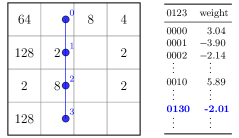
Fig 2: A straight $4$-tuple on a $2048$ board. According to the values in its lookup table, for the given board state it returns $-2.01$, since the empty square is encoded as $0$, the square containing $2$ as $1$, and the square containing $8$ as $3$.

For brevity, we will write $V_{i}[s]$ to denote $V_{i}[index_{i}(s)]$. With this notation Eq. 3 boils down to

$$V(s)=\sum_{i=1}^{m}V_{i}[s].$$

An $n$-tuple network is, in principle, a linear approximator, but is based on highly nonlinear features (lookup tables). The number of parameters of the $n$-tuple network is $O(mc^{n})$, where $m$ is the number of n-tuples, and $n$ is the size of the largest of them. Thus, it can easily involve millions of parameters since its number grows exponentially with $n$. At the same time, however, the state evaluation is quick, since the algorithm defined in Eq. 3 is only $O(mn)$, which make it one of the biggest advantages of $n$-tuple networks over more complex function approximators such as artificial neural networks. In practice, the largest factor influencing the performance of the $n$-tuple network evaluation is the memory accesses ($s[loc_{ij}]$), which is why we neglect (usually very small) $n$ and can claim the time complexity to be $O(m)$.

IV-B2 $n$-Tuple Network for $2048$

In $2048$, there are $18$ tile values, as the tile $2^{17}$ is, theoretically, possible to obtain. However, to limit the number of weights in the network, we assume $c=16$.

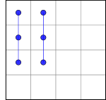
(a) a straight $3$-tuple shape

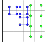
(b) $4$-tuple shapes: $4$ and $22$

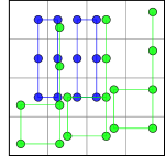
(c) $6$-tuple shapes: $33$ and $42$

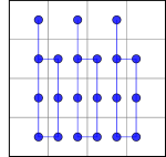
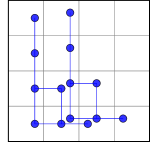
(d) $7$-tuple shapes: $43$ and $421$

Fig 3: $n$-tuple shapes considered in this paper. For clarity, the symmetric expansions were not shown.

Following Wu et al. [38], as our baseline function approximator, we use $33$-$42$ network shown in Fig. 3c. Its name corresponds to the shapes of tuples used. The network consists of four $6$-tuples, which implies $4\times 16^{6}=67\,108\,864$ parameters to learn.

Following earlier works on $n$-tuple networks [15, 23, 12], we also make advantage of symmetric sampling, which is a weight sharing technique allowing to exploit the symmetry of the board. In symmetric sampling, each $n$-tuple is employed eight times for each possible board rotation and reflection. Symmetric sampling facilitates generalization and improves the overall performance of the learning system without the expense of increasing the size of the model [31].

IV-C Temporal Difference Learning

Temporal Difference (TD) Learning is a basic but effective state-value function-based method to solve reinforcement learning problems. Reinforcement learning problem is an unknown MDP, in which the learning agent does not know the transition function or the reward function. This is not the case in 2048, where all the game mechanics are given in advance, but TD is perfectly applicable and has been successful also for known MDPs.

TD updates the state-value function $V_{\theta}$ in response to the current and next state, agent’s action and its immediate consequences. Assuming that an agent achieved state $s_{t+1}$ and reward $r_{t+1}$ by making an actions $a_{t}$ in state $s_{t}$, the TD($\lambda$) rule uses gradient descent to update $\theta$ in the following way:

$$\theta_{t+1}\leftarrow\theta_{t}+\alpha\delta_{t}\sum_{k=1}^{t}\lambda^{t-k}\nabla_{\theta_{k}}V_{\theta_{k}}(s_{k}),$$ (4)

where the prediction error $\delta_{t}=r_{t+1}+V_{\theta_{t}}(s_{t+1})-V_{\theta_{t}}(s_{t})$, $\alpha$ is the learning rate, and $\lambda\in[0,1]$ is the decay parameter which determines how much of the prediction error should be back-propagated to previously visited states.

A special case is when $\lambda=0$. Under a convenient assumption that $0^{0}\equiv 1$, the resulting rule, called TD($0$), boils down to:

$$\theta_{t+1}\leftarrow\theta_{t}+\alpha\delta_{t}\nabla_{\theta_{t}}V_{\theta_{t}}(s_{t}).$$

IV-D Afterstate Learning Framework with $n$-Tuple Networks

An agent to make a decision has to evaluate all possible states it can get into (cf. Eq. 2). In $2048$, there can be maximally $30$ such states, which can lead to a serious performance overhead.

In the previous work [31], we have shown that for $2048$, in order to reduce this computational burden, one can exploit the concept of afterstates, which are encountered in some MDP domains. An afterstate, denoted here as $s^{\prime}$, is a state reached after the agent’s action is made, but before a random element is applied. In 2048, it is the board position obtained immediately after sliding (and merging) the tiles. This process can be shown graphically:

$$s^{\prime}_{t}\xrightarrow{\textrm{random}}s_{t}\xrightarrow{a_{t}}s^{\prime}_{t+1}\xrightarrow{\textrm{random}}s_{t+1}.$$

The TD($\lambda$) rule for learning the afterstate-value does not change except the fact that it involves experience tuples of $(s^{\prime}_{t},a_{t},r_{t+1},s^{\prime}_{t+1})$ instead of $(s_{t},a_{t},r_{t+1},s_{t+1})$, where $r_{t+1}$ is a reward awarded for reaching state $s^{\prime}_{t+1}$.

The baseline afterstate learning framework using TD($\lambda$) rule and n-tuple network function approximator is presented in Alg. 1. The agent learns from episodes one by one. Each learning episode starts from an initial state obtained according to the game specification and ends when the terminal criterion is met (line $9$). The agent follows a greedy policy w.r.t. the afterstate-value function. After determining the action that yields the maximum afterstate value (line $10$), the agent makes it, obtaining a reward $r_{t+1}$, an afterstate $s^{\prime}_{t+1}$ and the next state $s_{t+1}$. This information is then used to compute the prediction error $\delta_{t}$ and to backpropagate this error to afterstate $s^{\prime}_{t}$ and its predecessors (line $13$). Notice that in a special case when $s_{t}$ is a terminal state, the $\delta_{t}=-V(s^{\prime}_{t})$ (line $15$).

An implementation of the TD($\lambda$) update rule for the $n$-tuple network consisting of $m$ $n$-tuples is shown in lines $30$-$33$. The algorithm updates the $n$-tuple network weights involved in computing the value for state $s^{\prime}_{k}$, where $k=t\dots 1$. Since, the term $\lambda^{t-k}$ decreases with decreasing $k$, which yields negligible update values, for efficiency, we limited the update horizon to $h$ the most recently visited states. We used $h=\left\lceil\log_{\lambda}0.1\right\rceil-1$ in order to retain updates where the expression $\lambda^{t\text{\textminus}k}\geq 0.1$.

It is important to observe that a standard implementation of TD($\lambda$) involving eligibility traces [30] cannot be applied to an $n$-tuple network. The eligibility traces vector is of the same length as the weight vector. The standard Sutton’s implementation consists in updating all the elements of the vector at each learning step. This is computationally infeasible when dealing with hundreds of millions of weights. A potential solution would be to maintain only the traces for activated weights [36]. This method has been applied to Connect Four. Notice, however, that the number of activated weights during the episode depends on its length. While Connect Four lasts maximally $42$ moves, $2048$ may require several ten thousand moves. Thus, an implementation of TD($\lambda$) requires a limited update horizon to be efficient.For convenience, the learning rate $\alpha$ is scaled down by the number of $n$-tuples $m$ (line $33$). As a result, $\alpha$ is independent of the number of $n$-tuples in the network and it is easier to interpret: $\alpha=1.0$ is the maximum sensible value, since for $s^{\prime}_{t}$, it immediately reduces the prediction error $\delta_{t}$ to zero ($V_{t+1}(s^{\prime}_{t})\leftarrow r_{t+1}+V_{t}(s^{\prime}_{t+1})$).

This learning framework does not include exploration, i.e., making non-greedy actions. Despite experimenting with $\epsilon$-greedy, softmax, and other custom exploration ideas, we found out that any non-greedy behavior significantly inhibits the agent’s ability to learn in the $2048$ game. Apparently, the inherently stochastic 2048 environment provides itself enough exploration.

1:function Learn

2:     while not enough learning do

3:         $s_{0}\leftarrow\textsc{InitialState}()$

4:         LearnFromEpisode($s_{0}$)      

5:end function

6:

7:function LearnFromEpisode($s_{0}$)

8:     $t=0$

9:     while not Terminal($s_{t}$) do

10:         $a_{t}\leftarrow\operatorname*{arg\,max}_{a\in A(s_{t})}\textsc{Evaluate}(s_{t},a_{t})$

11:         $r_{t+1},s^{\prime}_{t+1},s_{t+1}\leftarrow\textsc{MakeAction}(s_{t},a_{t})$

12:         if $t>0$ then

13:              TD($\lambda$)Update($r_{t+1}+V(s_{t+1}^{\prime})-V(s^{\prime}_{t})$)          

14:         $t\leftarrow t+1$      

15:     TD($\lambda$)Update($-V(s^{\prime}_{t})$)

16:end function

17:

18:function MakeAction($s,a$)

19:     $s^{\prime},r\leftarrow\textsc{GetAfterstate}(s,a)$

20:     $s^{\prime\prime}\leftarrow\textsc{AddRandomTile}(s^{\prime})$

21:     return $r,s^{\prime},s^{\prime\prime}$

22:end function

23:

24:function Evaluate($s,a$)

25:     $s^{\prime},r\leftarrow\textsc{GetAfterstate}(s,a)$

26:     return $r+V(s^{\prime})$

27:end function

28:

29:parameters: $\alpha,\lambda,h$

30:function TD($\lambda$)Update($\delta_{t}$)

31:     for $k=t\textbf{ downto }\max(t-h,1)$ do

32:         for $i=1\textbf{ to }m$ do

33:              $V_{i}[s^{\prime}_{k}]\leftarrow V_{i}[s^{\prime}_{k}]+\frac{\alpha}{m}\delta_{t}\lambda^{t-k}$               

34:end function

Algorithm 1 Framework for TD($\lambda$) learning afterstate-value $n$-tuple networks.

V Algorithms and Experiments

In this section, after presenting the common experimental setup, we introduce, one by one, some existing and several novel algorithms improving the afterstate learning framework introduced in Section IV.

V-A Experimental Setup

V-A1 Stopping Condition

In $2048$, the length of an episode highly depends on the agent’s competence, which increases with the number of learning episodes. This is why, in all the experiments in this paper, we limit the number of actions an agent can make during its lifetime instead of the number of episodes it can play. Unless stated otherwise, we give all the methods the same computational budget of $10^{10}$ actions, which corresponds to approximately $10^{7}$ learning episodes for the best algorithms.

V-A2 Performance Measures

We aimed at maximizing the expected score obtained by the agent. To monitor the learning progress, every $2\times 10^{8}$ actions, the learning agent played $1000$ episodes using the greedy policy w.r.t. value function. The average score we denote as $1$-ply performance. Since we were ultimately interested in combining the learned evaluation function with a tree search, we also regularly checked how the agent performs when coupled with expectimax [19, 24] of depth $3$ ($3$-ply performance). We played $300$ episodes for this purpose.

V-A3 Computational Aspects

All algorithms presented in this paper were implemented in Java. Experiments were executed on a machine equipped with two $2.4$ GHz AMD Opteron™ 6234 CPUs and $64$ GB RAM. In order to take advantage of its $24$ cores, we applied the lock-free optimistic parallelism, reducing the learning time by a factor of $24$ comparing to the single-threaded program.

Lock-free optimistic parallelism consists in letting all $24$ threads play and learn $2048$ in parallel using shared data without any locks. Since all threads simultaneously read from and write to the same $n$-tuple network lookup tables, in theory, race conditions can occur. In practice, however, since the $n$-tuple network can involve millions of parameters, the probability of a race condition is negligible, and we have not observed any adverse effects of this technique.

Even with the parallelization, however, a single $2048$ learning run takes, depending on the algorithm, $1$–$7$ days to complete. Thus, for statistics, we could repeat each algorithm run only $5$ times.

V-B Automatic Adaptive Learning Rate

One of the most critical parameters of temporal difference learning is the learning rate $\alpha$, which is hard to setup correctly by hand. This is why several algorithms that automatically set the learning rate and adapt it over time have been proposed. For linear function approximation, the list of online adaptive learning algorithms include Beal’s Temporal Coherence ([3]), Dabney’s $\alpha$-bounds [9], Sutton’s IDBD [29], and Mahmood’s Autostep [16]. A thorough comparison of these and other methods has recently been performed by Bagheri et al. [2] on Connect 4. It was shown that, while the learning rate adaptation methods clearly outperform the standard TD, the difference between them is not substantial, especially, in the long run. That is why we evaluated only two of them here: the simplest Temporal Coherence (TC($\lambda$)) [3] and the advanced, tuning-free Autostep , which was among the best methods not only for Connect 4 but also for Dot and Boxes [35]. . Both of them, not only adjust the learning rate automatically but maintain separate learning rates for each learning parameter.

V-B1 TC($\lambda$)

1:parameters: $\beta,\lambda,h$

2:function TC($\lambda$)Update($\delta_{t}$)

3:     for $k=t\textbf{ downto }\max(1,t-h)$ do

4:         for $i=1\textbf{ to }m$ do

5:              $\alpha_{i}=\begin{cases}\frac{\left|E_{i}[s^{\prime}_{k}]\right|}{A_{i}[s^{\prime}_{k}]},&\text{if }A_{i}[s^{\prime}_{k}]\neq 0\\ 1,&\text{otherwise }\end{cases}$

6:              $V_{i}[s^{\prime}_{k}]\leftarrow V_{i}[s^{\prime}_{k}]+\beta\frac{\alpha_{i}}{m}\delta_{t}\lambda^{t-k}$

7:              $E_{i}[s^{\prime}_{k}]\leftarrow E_{i}[s^{\prime}_{k}]+\delta_{t}$

8:              $A_{i}[s^{\prime}_{k}]\leftarrow A_{i}[s^{\prime}_{k}]+\left|\delta_{t}\right|$               

9:end function

Algorithm 2 TC($\lambda$) for the $n$-tuple network function approximator.

Algorithm 2 shows the TC($\lambda$)Update function which implements TC($\lambda$), replacing the TD($\lambda$)Update in Alg. 1. Except the afterstate-values function $V$, the algorithm involves two other functions: $E$ and $A$. For each afterstate $s^{\prime}$, they accumulate the sum of errors and the sum of absolute of errors, respectively (lines $7$-$8$). Initially, the learning rate is $1$ for each learning parameter ($E[s^{\prime}]=A[s^{\prime}]=0$). Then it is determined by the expression $\left|E_{i}[s^{\prime}]\right|/A_{i}[s^{\prime}]$ and will stay high when the two error accumulators have the same sign. When the signs start to vary, the learning rate decreases. TC($\lambda$) involves a meta-learning rate parameter $\beta$ (line 5). As with $\alpha$ for TD($\lambda$), since we scale down the expression by the number of $n$-tuples $m$, $\beta\in[0,1]$.

For $E$ and $A$ we use $n$-tuple networks of the same architecture as $V$.

V-B2 Autostep

Autostep [16] also uses separate learning rates for each function approximator weight, but it updates it in a significantly more sophisticated way than TC. Autostep extends Sutton’s IDBD [29] by normalizing the step-size update, setting an upper bound on it, and reducing the step-size value when detected to be large. It has three parameters: the meta-learning rate $\mu$, discounting factor $\tau$, and initial step-size $\alpha_{init}$. Our implementation of Autostep strictly followed the original paper [16].

V-B3 Results

In the computational experiment, we evaluated three methods: TD($\lambda$), TC($\lambda$) and Autostep, which differ by the number of parameters. Due to the computational cost of the learning, we were not able to systematically examine the whole parameter space and concentrated on the learning rate $\alpha$ for TD($\lambda$), meta learning rate $\beta$ for TD($\lambda$) and $\mu$ parameter for Autostep. Other choices were made in result of informal preliminary experiments.

In these experiments, for TD($\lambda$) and TC($\lambda$), we found that $\lambda=0.5$, $h=3$ work the best. Note that Autostep($\lambda$) has not been defined by its authors, thus we used $\lambda=0$. We also set $\alpha_{init}=1.0$ and $\tau=0.0001$, but found out that the algorithm is robust to the two parameters, which complies with its authors’ claims [16].

Table I shows the results of the computational experiment. The results indicate that, as expected TD($0.5$) is sensitive to $\alpha$. Although TC($\lambda$) and Autostep automatically adapt the learning rates, the results show that they are still significantly susceptible to meta-learning parameters.

Figure 4 presents the comparison of the learning dynamics for the best parameters found for the three algorithms considered. Clearly, the automatic adaptation outperforms the baseline TD($0.5$). Out of the two automatic learning rate adaptation methods, the simple TC($0.5$) works better than the significantly more sophisticated Autostep. Autostep starts as sharply as TC($0.5$), but then the learning dynamics slows down considerably. Autostep is also characterized by the higher variance (see the transparent bands). The poor performance of Autostep might be due to the fact that it has been formulated only for supervised (stationary) tasks and reinforcement learning for $2048$ makes the training data distribution highly non-stationary.

One disadvantage of both TC and Autostep is that since they involve more $n$-tuple networks (e.g., for $E$ and $A$), they need more memory access and thus increase the learning time. In our experiments Autostep and TC($0.5$) took roughly $2$ and $1.5$ times more to complete than TD($0.5$). However, the performance improvements shown in Fig. 4 are worth this overhead.

Table I: Influence of the (meta-)learning rate parameters on the averages scores obtained by controllers trained by TD($0.5$), TC($0.5$) and Autostep($0$) depending on the search depth ($1$- or $3$-ply).

$\alpha$	$1$-ply	$3$-ply
$0.01$	$41\,085$ p m 265	$99\,015$ p m 1318
$0.1$	$102\,130$ p m 1287	$175\,301$ p m 1946
$0.5$	$130\,266$ p m 2136	$196\,138$ p m 3864
$1.0$	$141\,456$ p m 1050	$237\,026$ p m 8081

(a) TD($0.5$)

$\beta$	$1$-ply	$3$-ply
$0.1$	$200\,588$ p m 1581	$292\,558$ p m 4856
$0.5$	$244\,905$ p m 3811	$335\,076$ p m 1639
$1.0$	$250\,393$ p m 3424	$333\,010$ p m 2856

(b) TC($0.5$)

$\mu$	$1$-ply	$3$-ply
$0.001$	$90\,758$ p m 1789	$146\,171$ p m 1023
$0.01$	$152\,737$ p m 6573	$249\,609$ p m 13142
$0.1$	$171\,396$ p m 6662	$246\,740$ p m 15469
$0.4$	$156\,112$ p m 8788	$200\,391$ p m 18425
$0.7$	$33\,490$ p m 726	$66\,557$ p m 659
$1.0$	$2546$ p m 62	$5889$ p m 157

(c) Autostep with $\alpha_{init}=1.0$, $\tau=0.0001$

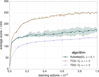
(a) Performance at $1$-ply

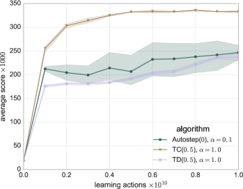
(b) Performance at $3$-ply

Figure 4: Comparison of the learning dynamics of TD($0.5$) with $\alpha=1.0$, TC($0.5$) with $\beta=1.0$, and Autostep($0$) with $\mu=0.1$. The transparent bands mean the $95\%$ confidence interval.

V-C Delayed Temporal Difference

We have observed that the computational bottleneck of the learning process lies in the access to the $n$-tuples lookup tables. This is because the lookup tables are large and do not fit into the CPU cache. In the TD($\lambda$) implementation presented in Alg. 1), the number of lookup table accesses is $O(mh)$, where $m$ is the number of $n$-tuples and $h$ is the update horizon (lines $30$–$33$).This is because in each step $t$, the current prediction error $\delta_{t}$ is used to update the weights that were active during the $h+1$ last states. Thus, each weight active in a given state is updated $h+1$ times until the state falls beyond the horizon. Notice, that the cumulative error used as the update signal is a weighted sum of $h+1$ subsequent prediction errors, i.e., $\Delta_{t}=\sum_{k=0}^{h}\delta_{t+k}\lambda^{k}$. Our novel algorithm, delayed-TD($\lambda$), removes the dependency on $h$.It operates as follows.

Delayed-TD($\lambda$) stores the last $h+1$ states $s_{t}$ and errors $\delta_{t}$. Instead of instantly updating the weights active in state $s_{t}$, it delays the update by $h$ steps. Then it updates the weights by the (decayed) cumulative error $\Delta_{t-h}$. This way, the weights active in a given visited state are updated only once. Since the vector of stored errors $\delta_{t}$ constitutes a small, continuous memory block, it fits in the processor cache. It makes its access time negligible compared to the time required to access the main memory in which the large $n$-tuple network lookup tables reside.

1:parameters: $\alpha,\lambda,h$

2:function DelayedTD($\lambda$)Update($\delta_{t}$)

3:     if $t>h$ then

4:         $\Delta_{t-h}=\sum_{k=0}^{h}{\delta_{t-h+k}\lambda^{k}}$

5:         ActualTDUpdate($s^{\prime}_{t-h},\Delta_{t-h}$)      

6:end function

7:

8:function Finally

9:     for $h^{\prime}=h-1\textbf{ downto }0\ \textbf{do}$

10:         $\Delta_{t-h^{\prime}}=\sum_{k=0}^{h^{\prime}}{\delta_{t-h^{\prime}+k}\lambda^{k}}$

11:         ActualTDUpdate($s^{\prime}_{t-h^{\prime}},\Delta_{t-h}$)      

12:end function

13:

14:function ActualTDUpdate($s^{\prime},\Delta$)

15:     for $i=1\textbf{ to }m$ do

16:         $V_{i}[s^{\prime}]\leftarrow V_{i}[s^{\prime}]+\frac{\alpha}{m}\Delta$      

17:end function

Algorithm 3 Delayed-TD($\lambda$) for $n$-tuple network. The function Finally must be executed as the last statement in the LearnFromEpisode function in Alg. 1.

1:parameters: $\beta,\lambda,h$

2:function ActualTCUpdate($s^{\prime},\Delta$)

3:     for $i=1\textbf{ to }m$ do

4:         $\alpha_{i}=\begin{cases}\frac{\left|E_{i}[s^{\prime}]\right|}{A_{i}[s^{\prime}]},&\text{if }A_{i}[s^{\prime}]\neq 0\\ 1,&\text{otherwise }\end{cases}$

5:         $V_{i}[s^{\prime}]\leftarrow V_{i}[s^{\prime}]+\beta\frac{\alpha_{i}}{m}\Delta$

6:         $E_{i}[s^{\prime}]\leftarrow E_{i}[s^{\prime}]+\Delta$

7:         $A_{i}[s^{\prime}]\leftarrow A_{i}[s^{\prime}]+\left|\Delta\right|$      

8:end function

Algorithm 4 Delayed-TC($\lambda$) for the $n$-tuple network. The functions DelayedTC($\lambda$), Update($\delta_{t}$) and Finally are analogous to the ones used in delayed-TD($\lambda$) in Alg. 3.

The delayed versions of TD($\lambda$) and TC($\lambda$) are shown in Alg. 3 and 4. Notice that since the actual update is delayed, it is done only when $t>h$. Also, when the episode is finished, the algorithm needs to take care of the most recently visited states. To this aim, the Finally function is executed as the last statement in the LearnFromEpisode function (Alg. 1).

Table II: Delayed vs. standard versions of temporal difference algorithms. We used $h=3$ and $\alpha=1.0$ for TD($0.5$) and $\beta=1.0$ for TC($0.5$). The averages are accompanied by the $95\%$ confidence interval.

algorithm	$1$-ply	$3$-ply	time [days]
TD(0.5)	$140\,397$ p m 1974	$234\,997$ p m 4717	$0.26$ p m 0.01
delayed-TD(0.5)	$141\,456$ p m 1050	$237\,026$ p m 8081	$0.23$ p m 0.01
TC(0.5)	$248\,770$ p m 2296	$333\,010$ p m 2856	$1.16$ p m 0.03
delayed-TC(0.5)	$250\,393$ p m 3424	$335\,580$ p m 6299	$0.39$ p m 0.01

The delayed temporal difference can be seen as a middle-ground between the online and offline temporal difference rules [30]. The computational experiment results shown in Table II reveal no statistically significant differences between the standard and delayed versions of temporal difference algorithms. On the other hand, as expected, the delayed versions of the algorithms are significantly quicker. Delayed-TC($0.5$) is roughly $3$ times more effective than the standard TC($0.5$). The difference for TD($0.5$) is minor because the weight update procedure is quick anyway and it is dominated by the action selection (line $10$ in Alg. 1). In all the following experiments we will use the delayed version of TC($0.5$).

V-D Multi-Stage Weight Promotion

V-D1 Stages

To further improve the learning process, we split the game into stages and used a separate function approximator for each game stage. This method has been already used in Buro’s Logistello [6], a master-level Othello playing program, and its variant with manually selected stages has already been successfully applied to 2048 [38]. The motivation for multiple stages for $2048$ results from the observation that in order to precisely approximate the state-value function, certain features should have different weights depending on the stage of the game. The game has been split into $2^{g}$ stages, where $g$ is a small positive integer. Assuming that the maximum tile to obtain in $2048$ is $2^{15}=32\,768$, the “length” of each stage is $l=2^{15+1-g}$. When $g=4$, $l=2^{12}=4096$. In this example, the game starts in stage $0$ and switches to stage $1$ when $4096$-tile is achieved, stage $2$ on $8192$-tile, stage $3$ when both $8192$ and $4096$ are on the board, stage $4$ on $16\,384$, and so on.

The value function for each stage is a separate $n$-tuple network. Thus, introducing stages makes the model larger by a factor of $2^{g}$. Thus, if $g=4$, the $33$-$42$ network requires $2^{4}\times 4\times 6^{16}=1\,073\,741\,824$ parameters.

We also need the multi-stage versions of $E$ and $A$ functions in TC($\lambda$) algorithm, thus lines $5$-$7$ of Alg. 2 become:

5:$V^{stage(s^{\prime})}_{i}[s^{\prime}]\leftarrow V^{stage(s^{\prime})}_{i}[s^{\prime}]+\beta\frac{\alpha_{i}}{n}\Delta$

6:$E^{stage(s^{\prime})}_{i}[s^{\prime}]\leftarrow E^{stage(s^{\prime})}_{i}[s^{\prime}]+\Delta$

7:$A^{stage(s^{\prime})}_{i}[s^{\prime}]\leftarrow A^{stage(s^{\prime})}_{i}[s^{\prime}]+\left|\Delta\right|$.

V-D2 Weight Promotion

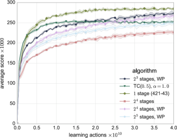
(a) $1$-ply performance

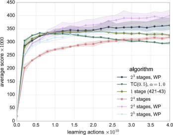
(b) $3$-ply performance

Figure 5: The effects of multiple stages and weight promotion on learning performance.

Table III: Performance of algorithms involving multiple stages and weight promotion (“WP”) after $4\times 10^{10}$ actions. All except the “$1$ stage $421$-$43$” variant used the $42$-$33$ network, trained with delayed-TC($0.5$), $\alpha=1.0$.

algorithm	$1$-ply	$3$-ply	time [days]
1 stage	$251\,033$ p m 3483	$296\,207$ p m 4613	$1.62$
$2^{4}$ stages	$226\,352$ p m 5433	$318\,534$ p m 4154	$2.22$
$2^{3}$ stages, WP	$273\,510$ p m 3012	$363\,379$ p m 25276	$2.18$
$2^{4}$ stages, WP	$267\,544$ p m 3707	$400\,124$ p m 21739	$2.24$
$2^{5}$ stages, WP	$250\,051$ p m 4790	$355\,413$ p m 10350	$2.42$
1 stage, $421$-$43$	$284\,657$ p m 4605	$326\,267$ p m 2678	$1.76$

The initial experiments with the multi-stage approximator revealed that increasing the model by using the multi-stage approach actually harms the learning performance. This is because, for each stage, the $n$-tuple network must learn from scratch. As a result, the generalization capabilities of the multi-stage function approximator are significantly limited. In order to facilitate generalization without removing the stages, we initialize each weight, upon its first access, to the weight of the corresponding weight in the preceding stage (the weight from a given stage is “promoted” to the subsequent one). To implement this idea, the following lines are added in the Evaluate function between lines $25$ and $26$ of Alg. 1:

26:if $V^{stage(s^{\prime})}_{i}[s^{\prime}]$ not accessed and $stage(s^{\prime})>0$ then

27:     $V_{i}^{stage(s^{\prime})}[s^{\prime}]\leftarrow V_{i}^{stage(s^{\prime})-1}[s^{\prime}]$

In order to avoid adding additional data structures (memory and performance hit), we implement the condition in line $21$ as checking whether $V_{i}^{stage(s^{\prime})}[s^{\prime}]$ equals $0$, heuristically assuming that $V_{i}^{stage(s^{\prime})}[s^{\prime}]=0$ until the first access.

V-D3 Results

In order to evaluate the influence of the multi-stage approximator and weight promotion, we performed a computational experiment with six algorithm variants.

The results, shown in Table III and Fig. 5, indicate that the multi-stage approximator involving $2^{4}$ stages actually slows down the learning compared to the single stage baseline. This is generally true for both $1$-ply and $3$-ply, but at $3$-ply, the $2^{4}$-stages approximator, eventually, outperforms the $1$-stage baseline. However, Fig. 5 shows that it is due to the drop of performance of the $1$-stage approximator rather than to the increase of the learning performance of the multi-stage approach. After $1\times 10^{10}$ actions, the $1$-stage approximator’s $3$-ply performance starts to decrease due to overfitting to $1$-ply settings, which is used during the learning.

Essential to defeat the $1$-stage baseline is the weight promotion. Although the algorithm variants with weight promotion still learn at a slower pace than the baseline, they eventually outperform it regardless of the search tree depth.

What is the optimal number of stages? The answer to this question depends on the depth at which the agent is evaluated. The results show that $2^{5}$ stages is overkill since it works worse than $2^{4}$ and $2^{3}$ stages. The choice between $2^{3}$ and $2^{4}$ is not evident, though. For $1$-ply, the approximator involving $2^{3}$ stages learns faster and achieves a slightly better performance than the one with $2^{4}$ stages. But for $3$-ply the situation is opposite and $2^{4}$ clearly excels over $2^{3}$. Since we are interested in the best score in absolute terms, we favor the $2^{4}$ stages variant.

More stages involve more parameters to learn. As we already stated, $2^{4}$ stages imply $16$ times more parameters than the $1$-stage baseline. Is there a better way to spent the parameter budget? In order to answer this question, we constructed a large single stage $421$-$43$ network containing $5$ $7$-tuples of two shapes shown in Fig. 3d. The network is of a similar size to the $2^{4}$ stages $42$-$33$ network, involving $5\times 16^{7}=1\,342\,177\,280$ weights. Fig. 5 reveals that the new network indeed excels at $1$-ply, but performs poorly at $3$-ply. Interestingly, at $3$-ply, it not only does not improve over the $42$-$33$ network but it also suffers from the $1$-ply overfitting syndrome as it was the case with the $1$-stage baseline.

Thus, it is tempting to conclude that multi-stage approximators are immune to the $1$-ply overfitting syndrome. Notice, however, that the overfitting happens only after the process converges and neither of the multi-stage variants has converged yet.

Our best setup at $3$-ply involving $2^{4}$ stages and weight promotion significantly improved over the $1$-stage baseline. Although, neither the number of stages nor the weight selection did not negatively influence the learning time, the new algorithm was found to require $4$ times more actions to converge (and it still exhibits some growth potential).

V-E Carousel Shaping and Redundant Encoding

As we have seen in the previous section, the $1$-ply performance does not always positively correlate with the $3$-ply performance. Some algorithms exhibit an overfitting to $1$-ply settings — the better an agent gets at $1$-ply, the worse it scores at $3$-ply.

V-E1 Carousel Shaping

Here we deal with $1$-ply overfitting by introducing carousel shaping, which concentrates the learning effort on later stages of $2048$. This is motivated by the fact that only a small fraction of episodes gets to the later stages of the game. Carousel shaping tries to compensate this. Accurate estimates of the later stages of the game are particularly important for $k$-ply agents, where $k>1$, since they can look ahead further than the $1$-ply ones.

In carousel shaping, we use the notion of an initial state of a stage. Any game’s initial state is an initial state of stage $1$. If two subsequent states $s^{\prime}_{t-1}$, and $s^{\prime}_{t}$ such that $stage(s^{\prime}_{t-1})+1=stage(s^{\prime}_{t})$, $s^{\prime}_{t}$ is an initial stage of $stage(s^{\prime}_{t})$. A set of the last $1000$ visited initial states of each stage is maintained during the learning.

The carousel shaping algorithm starts from an initial state of stage $1$ After each learning episode, it proceeds to the subsequent stage. It starts each episode with a randomly selected initial state of the current stage. It restarts from stage $1$, when it hits an empty set of initial states (see Alg. 5). This way, the learning more often visits the later stages of the game.

Note that this technique is different from the one introduced for $2048$ by Wu et al. [38]. Their algorithm learns the n-tuple networks stage by stage. After some number of learning episodes for a given stage, it moves to the next one and never updates the weights for the previous one again. The state-value function learned this way may not be accurate. New information learned in a given stage does not backpropagate to the previous stages. This might lead to suboptimal behavior.

1:function CarouselShaping

2:     $stage\leftarrow 1$

3:     $initstates[x]=\emptyset$ for $x\in\{1\dots 2^{g}\}$

4:     while not enough learning do

5:         if $stage=1$ then

6:              $s\leftarrow\textsc{InitialState}()$

7:         else

8:              $s\leftarrow\textsc{RandomChoice}(initstates[stage])$          

9:         LearnFromEpisode($s$) $\triangleright$ Updates $initstates$

10:         $stage\leftarrow stage+1$

11:         if $stage>2^{g}$ or $initstates[stage]=\emptyset$ then

12:              $stage\leftarrow 1$               

13:end function

Algorithm 5 Carousel shaping.

V-E2 Redundant Encoding

The last technique we apply to $2048$ is redundant encoding. We define redundant encoding as additional features to the function approximator that does not increase its expressiveness. Although the new features are redundant from the point of view of the function approximator, they can facilitate learning by quicker generalization. For the $n$-tuple network, redundant encoding consists in adding smaller $n$-tuples, which are comprised in the larger ones. In our experiments, we first extended our standard $42$-$33$ network by $4$-tuples of two shapes: straight lines of length $4$ and $2\times 2$ squares denoted as “$22$”. Finally, we added straight lines of length $3$ (denoted as “$3$”) (see Fig. 3).

V-E3 Results

Table IV: Performance of algorithms involving carousel shaping (“CS”) and redundant encoding after $4\times 10^{10}$ actions. All variants used the $42$-$33$ network with $2^{4}$ stages and weight promotion, trained with delayed-TC($0.5$), $\alpha=1.0$.

algorithm	$1$-ply	$3$-ply	# $n$-tuples	time [days]
42-33 (baseline)	$265\,435$ p m 8511	$393\,289$ p m 26496	$5$	$2.35$
42-33, CS	$258\,616$ p m 5784	$432\,701$ p m 13005	$5$	$2.78$
42-33-4-22, CS	$256\,569$ p m 19975	$457\,754$ p m 6256	$10$	$4.63$
42-33-4-22-3	$319\,433$ p m 2708	$469\,779$ p m 10920	$12$	$5.06$
42-33-4-22-3, CS	$311\,426$ p m 9633	$491\,398$ p m 19458	$12$	$5.47$

The results of applying carousel shaping and redundant encoding are shown in Table. IV. Clearly, the effect of carousel shaping on $1$-ply performance is consistently slightly negative. This is less important, however, since we can see that the method significantly improves the $3$-ply performance regardless of the network architecture.

We can also see that the best algorithm involves the redundant $4$-tuples and $3$-tuples. Compared to the standard $42$-$33$ network, the redundant $4$-tuples do not help at $1$-ply, but they make a difference at $3$-ply. The redundant $3$-tuples show a significant improvement both at $1$- and $3$-ply. The figure also indicates that there is a synergetic effect of redundant encoding and carousel shaping, especially at $3$-ply, where the algorithm using both techniques scores nearly $500\,000$ points on average.

A downside of redundant encoding is that it makes the learning slower due to involving more $n$-tuples, which results in more table lookups for each state evaluation. Table IV shows that the learning time is roughly proportional to the number of $n$-tuples involved. Notice, however, that the redundant $n$-tuples are required only during the learning. After the learning is finished, the lookup tables corresponding to the redundant $n$-tuples can be integrated into the lookup tables of the n-tuples that contain the redundant ones. This way, the resulting agent has the same performance as if it was trained without redundant encoding.

VI The Best $n$-Tuple Network

VI-A Expectimax Tree Search

The best $n$-tuple network in the experiments has been obtained using TC($0.5$) with $\alpha=1.0$ with redundant encoding (the $42$-$33$-$22$-$4$-$3$ network), $2^{4}$ stages, with weight promotion, and carousel shaping. Here we evaluate it thoroughly.

Table V shows how the performance of the network depends on how deep expectimax it is allowed to search the game tree. For the experiment, the player was allowed to use either constant depth ($1$-ply, $2$-ply, $3$-ply, or $5$-ply) or constant time per move (iterative deepening with $1$ ms, $50$ ms, $100$ ms, $200$ ms or $1000$ ms). In the latter case, the agent could go deeper than $5$-ply if the time allows, which happen especially in the end-games, in which the branching factor gets smaller. Transposition tables were used to improve the performance of expectimax. The program was executed on Intel i7-4770K CPU @ $3.5$ GHz, single-threaded.

Table V shows that, generally, the deeper the search tree, the better its average score is. It is also clear, however, that the CPU time can be spent more effectively if we limit the time per move rather than the search tree depth (compare the results for $5$-ply vs. $100$ ms). We can also see that increasing the time per move allows to make better decisions, which renders in better scores.

VI-B Comparison with Other $2048$ Controllers

Table VI shows a performance comparison of our best controller with other published $2048$ players. Clearly, our player outperforms the rest. It is important to show how large the gap between our controller and the runner-up is (which, apart from hand-made features, also uses the $42$-$33$ network). Our $n$-tuple network outranks it regardless of the expectimax settings: at $100$ ms per move and $3$-ply depth (the Yeh et. al’s controller also uses $3$-ply). Moreover, our network is even slightly better than the runner-up at $2$-ply, when it can play more than $40$ times faster. This confirms the effectiveness of the learning methodology developed in this paper.

Table V: Performance of the best $n$-tuple network with respect to the search limit (constant depth or time limit per move).

Search limit	Average score	$32\,768$ [%]	$16\,384$ [%]	$8192$ [%]	# games	Moves/s
1-ply	$324\,710$ p m 11043	$19$	$68$	$90$	$1000$	$258\,371$
2-ply	$457\,079$ p m 11112	$34$	$91$	$99$	$1000$	$20\,524$
3-ply	$511\,759$ p m 12021	$50$	$92$	$99$	$1000$	$1484$
5-ply	$545\,833$ p m 21500	$54$	$97$	$100$	$300$	$16$
1 ms	$527\,099$ p m 11486	$54$	$95$	$100$	$1000$	$916$
50 ms	$576\,655$ p m 20839	$62$	$97$	$99$	$300$	$20$
100 ms	$589\,355$ p m 20432	$65$	$96$	$100$	$300$	$10$
200 ms	$591\,380$ p m 21870	$67$	$97$	$99$	$300$	$5$
1000 ms	$609\,104$ p m 38433	$70$	$97$	$98$	$100$	$1$

Table VI: Comparison with other methods.

Authors	Average score	$32\,768$ [%]	Moves/s	Method
Szubert & Jaśkowski [31]	$99\,916$	$0$	$330\,000$	$n$-tuple network, TD($0$), $1$-ply
Oka & Matsuzaki [21]	$234\,136$	$3$	$88\,000$	$n$-tuple network, TD($0$), $1$-ply
Wu et al. [38]	$328\,946$	$11$	$300$	multi-stage TD($0$), $3$-ply
Xiao et al. [39]	$442\,419$	$32$	$3$	hand-made features, CMA-ES, adaptive depth
Yeh et al. [40]	$443\,526$	$32$	$500$	$n$-tuple network, hand-made features, $3$-ply
This work	$324\,710$	$19$	$258\,371$	$n$-tuple network, $1$-ply
	$457\,079$	$34$	$20\,524$	$n$-tuple network, $2$-ply
	$511\,759$	$50$	$1464$	$n$-tuple network, $3$-ply
	$527\,099$	$54$	$916$	$n$-tuple network, $1$ ms/move
	$609\,104$	$70$	$1$	$n$-tuple network, $1000$ ms/move

VII Discussion and Conclusions

In this paper, we presented how to obtain a strong $2048$ controller. It scores more than $600\,000$ points on average and achieves the $32\,768$-tile in $70\%$ of games, which is significantly more than any other $2048$ computer program to date. It is also unlikely that any human player can achieve such level of play. At least because some episodes could require as much as $30\,000$ moves to finish, which makes human mistakes inevitable.

In order to obtain this result, we took advantage of several existing and introduced some new reinforcement learning techniques (see Table VII). First, we applied temporal coherence (TC) learning that turned out to significantly improve the strength of the player compared to the vanilla temporal difference (TD) learning. Second, we used a different function approximator for each stage of the game but have shown that it pays off only when additional generalization methods are applied. For this aim, we introduced the weight promotion technique. Third, we demonstrated that the controller can be further improved when carousel shaping is employed. It makes the “later” stages of the game visited more often. It worsens the controller at $1$-ply, but improves it at $3$-ply, which we really care about. Finally, it was the redundant encoding that boosted the learning effectiveness substantially. Redundant encoding facilitates generalization and, as a result, the learning speed and the final controller score. Although it slows the learning, the redundant $n$-tuples can be incorporated into the non-redundant ones when the learning is finished, making the final agent quicker.

Table VII: Summary of the performance improvements obtained by introducing subsequent techniques

algorithm	$1$-ply	$3$-ply	learning days
TD($0.5$)	$141\,456$ p m 1050	$237\,026$ p m 8081	$0.26$ p m 0.01
TC($0.5$)	$248\,770$ p m 2296	$333\,010$ p m 2856	$1.16$ p m 0.03
delayed-TC($0.5$)	$250\,393$ p m 3424	$335\,580$ p m 6299	$0.39$ p m 0.01
$+$ $2^{4}$ stages & Weight Promotion	$267\,544$ p m 3707	$400\,124$ p m 21739	$2.24$
$+$ Redundant Encoding	$319\,433$ p m 2708	$469\,779$ p m 10920	$5.06$
$+$ Carousel Shaping	$311\,426$ p m 9633	$491\,398$ p m 19458	$5.47$

We also showed some techniques to lessen the computational burden. We introduced delayed versions of the temporal difference update methods and demonstrated that it can reduce the learning time of temporal coherence (TC) several times making the state-value function update mechanism vastly independent of the decay parameter $\lambda$. Secondly, we proved the practical efficacy of the lock-free optimistic parallelism, which made it possible to utilize all CPU cores during the learning.

From the broader point of view, although we concentrated on a specific problem of the game $2048$, the techniques we introduced are general and can be applied to other discrete Markov decision problems, in which $n$-tuple networks or, more broadly, tile encodings, can be effectively used for function approximation.

In this context, it is worth to emphasize the role of the (systematic) $n$-tuple networks for the overall result. Although they do not scale up to state spaces with large dimensionality [13], they have undeniable advantages for state spaces of moderate sizes and dimensions. They provide nonlinear transformations and computational efficiency. As we demonstrated, $n$-tuple networks can have billions of parameters, but at the same time, only a tiny fraction of them is involved to evaluate a given state or to update the state-value function. On the one hand, the enormous number of parameters of $n$-tuple network can be seen as a disadvantage as it requires a vast amount of computer memory. On the other hand, this is also the reason that the lock-free optimistic parallelism can work seamlessly.

From the $2048$ perspective, this work can be extended in several directions. First of all, although $n$-tuple networks allowed us to obtain a very competent $2048$ player, we believe they do not generalize too well for this problem. They rather learn by heart. Humans generalize significantly better. For example, for two board states, one of which has tiles with doubled values, a human player would certainly use similar, if not the same, strategy. Our $n$-tuple network cannot do that. This is why the learning takes days. So the open question is, how to design an efficient state-value function approximator that generalizes better? Actually, it is not clear whether this is possible at all since for the above example a state-value approximator is supposed to return two different values. We speculate that better generalization (and thus, faster learning) for $2048$ may require turning away from state-value functions and learning policies directly. A directly learned policy does not need to return numbers that have absolute meaning, thus, in principle, can generalize over to the boards mentioned in the example.

The second direction to improve the $2048$ controller performance involves including some hand-designed features. Although local features would probably not help since the $n$-tuple networks involve all possible local features, what our function approximator lacks are global features like the number of empty tiles on the board.

Some of the introduced techniques could also be improved or fine-tuned at least. For example, we did not experiment with carousel shaping. It is possible to parametrize it in order to control how much it puts the learning attention to the “later” stages. The question about how to effectively involve exploration is also open. No exploration mechanism we tried worked, but the lack of exploration may, eventually, make the learning prone to stuck in local minima, so an efficient exploration for $2048$ is another open question. Moreover, the learning rate adaptation mechanism of temporal coherence is somewhat trivial and arbitrary. Since the more sophisticated Autostep failed, there can be an opportunity for a new learning rate adaptation method.

Last but not least, we demonstrated how the learned evaluation function can be harnessed by a tree search algorithm. We used the standard expectimax with iterative deepening with transposition tables, but some advanced pruning [26] could potentially improve its performance.

Acknowledgments

The author thank Marcin Szubert for his comments to the manuscript and Adam Szczepański for implementing an efficient C++ version of the $2048$ agent. This work has been supported by the Polish National Science Centre grant no. DEC-2013/09/D/ST6/03932. The computations were performed in Poznan Supercomputing and Networking Center.

References

- [1] James S Albus. A theory of cerebellar function. Mathematical Biosciences, 10(1):25–61, 1971.
- [2] S Bagheri, M Thill, P Koch, and W Konen. Online Adaptable Learning Rates for the Game Connect-4. Computational Intelligence and AI in Games, IEEE Transactions on, 8(1):33–42, 2016.
- [3] Don F Beal and Martin C Smith. Temporal coherence and prediction decay in TD learning. In Proceedings of the 16th International Joint Conference on Artificial Intelligence, volume 1, pages 564–569. Morgan Kaufmann Publishers Inc., 1999.
- [4] Marc G Bellemare, Yavar Naddaf, Joel Veness, and Michael Bowling. The arcade learning environment: An evaluation platform for general agents. Journal of Artificial Intelligence Research, 2012.
- [5] Woodrow Wilson Bledsoe and Iben Browning. Pattern recognition and reading by machine. In Proc. Eastern Joint Comput. Conf., pages 225–232, 1959.
- [6] Michael Buro. Logistello: A Strong Learning Othello Program. In 19th Annual Conference Gesellschaft für Klassifikation e.V., 1995.
- [7] Michael Buro. From Simple Features to Sophisticated Evaluation Functions. In Proceedings of the First International Conference on Computers and Games, pages 126–145, London, UK, 1999. Springer.
- [8] Lucian Buşoniu, Robert Babuška, Bart De Schutter, and Damien Ernst. Reinforcement Learning and Dynamic Programming Using Function Approximators. CRC Press, Boca Raton, Florida, 2010.
- [9] William Dabney and Andrew G Barto. Adaptive Step-Size for Online Temporal Difference Learning. In AAAI, 2012.
- [10] Nikolaus Hansen and Andreas Ostermeier. Completely derandomized self-adaptation in evolution strategies. Evolutionary computation, 9(2):159–195, 2001.
- [11] Wojciech Jaśkowski. Systematic n-tuple networks for othello position evaluation. ICGA Journal, 37(2):85–96, June 2014.
- [12] Wojciech Jaśkowski and Marcin Szubert. Coevolutionary CMA-ES for knowledge-free learning of game position evaluation. IEEE Transactions on Computational Intelligence and AI in Games, (accepted), 2016.
- [13] Wojciech Jaśkowski, Marcin Szubert, Paweł Liskowski, and Krzysztof Krawiec. High-dimensional function approximation for knowledge-free reinforcement learning: a case study in SZ-Tetris. In GECCO’15: Proceedings of the 17th annual conference on Genetic and Evolutionary Computation, pages 567–574, Mardid, Spain, July 2015. ACM, ACM Press.
- [14] Leslie Pack Kaelbling, Michael L Littman, and Andrew W Moore. Reinforcement learning: A survey. Journal of artificial intelligence research, pages 237–285, 1996.
- [15] Simon M. Lucas. Learning to play Othello with N-tuple systems. Australian Journal of Intelligent Information Processing Systems, Special Issue on Game Technology, 9(4):01–20, 2007.
- [16] Ashique Rupam Mahmood, Richard S Sutton, Thomas Degris, and Patrick M Pilarski. Tuning-free step-size adaptation. In Acoustics, Speech and Signal Processing (ICASSP), 2012 IEEE International Conference on, pages 2121–2124. IEEE, 2012.
- [17] Edward P. Manning. Using Resource-Limited Nash Memory to Improve an Othello Evaluation Function. IEEE Transactions on Computational Intelligence and AI in Games, 2(1):40–53, 2010.
- [18] Rahul Mehta. 2048 is (PSPACE) Hard, but Sometimes Easy. arXiv preprint arXiv:1408.6315, 2014.
- [19] Donald Michie. Game-playing and game-learning automata. Advances in programming and non-numerical computation, pages 183–200, 1966.
- [20] Todd W Neller. Pedagogical possibilities for the 2048 puzzle game. Journal of Computing Sciences in Colleges, 30(3):38–46, 2015.
- [21] Kazuto Oka and Kiminori Matsuzaki. Systematic selection of n-tuple networks for 2048. In International Conference on Computers and Games (CG 2016), Leiden, The Netherlands, 2016.
- [22] Philip Rodgers and John Levine. An investigation into 2048 AI strategies. In Computational Intelligence and Games (CIG), 2014 IEEE Conference on, pages 1–2. IEEE, 2014.
- [23] Thomas Runarsson and Simon Lucas. Preference Learning for Move Prediction and Evaluation Function Approximation in Othello. Computational Intelligence and AI in Games, IEEE Transactions on, 6(3):300–313, 2014.
- [24] S.J. Russell, P. Norvig, J.F. Canny, J.M. Malik, and D.D. Edwards. Artificial intelligence: a modern approach, volume 74. Prentice hall Englewood Cliffs, NJ, 1995.
- [25] Arthur L. Samuel. Some Studies in Machine Learning Using the Game of Checkers. IBM Journal of Research and Development, 44(1):206–227, 1959.
- [26] Maarten PD Schadd, Mark HM Winands, and Jos WHM Uiterwijk. Chanceprobcut: Forward pruning in chance nodes. In Computational Intelligence and Games, 2009. CIG 2009. IEEE Symposium on, pages 178–185. IEEE, 2009.
- [27] Bruno Scherrer, Mohammad Ghavamzadeh, Victor Gabillon, Boris Lesner, and Matthieu Geist. Approximate Modified Policy Iteration and its Application to the Game of Tetris. Journal of Machine Learning Research, page 47, 2015.
- [28] David Silver, Aja Huang, Chris J Maddison, Arthur Guez, Laurent Sifre, George van den Driessche, Julian Schrittwieser, Ioannis Antonoglou, Veda Panneershelvam, Marc Lanctot, et al. Mastering the game of go with deep neural networks and tree search. Nature, 529(7587):484–489, 2016.
- [29] Richard S Sutton. Adapting bias by gradient descent: An incremental version of delta-bar-delta. In AAAI, pages 171–176, 1992.
- [30] Richard S. Sutton and Andrew G. Barto. Introduction to Reinforcement Learning. MIT Press, Cambridge, MA, USA, 1998.
- [31] Marcin Szubert and Wojciech Jaśkowski. Temporal difference learning of n-tuple networks for the game 2048. In IEEE Conference on Computational Intelligence and Games, pages 1–8, Dortmund, Aug 2014. IEEE.
- [32] Marcin Szubert, Wojciech Jaśkowski, and Krzysztof Krawiec. On scalability, generalization, and hybridization of coevolutionary learning: a case study for othello. IEEE Transactions on Computational Intelligence and AI in Games, 5(3):214–226, 2013.
- [33] Marcin G. Szubert, Wojciech Jaśkowski, and Krzysztof Krawiec. On Scalability, Generalization, and Hybridization of Coevolutionary Learning: A Case Study for Othello. IEEE Transactions on Computational Intelligence and AI in Games, 5(3):214–226, 2013.
- [34] Gerald Tesauro. Temporal difference learning and td-gammon. Communications of the ACM, 38(3):58–68, 1995.
- [35] Markus Thill. Temporal difference learning methods with automatic step-size adaption for strategic board games: Connect-4 and dots-and-boxes. Master’s thesis, Cologne Univ. of Applied Sciences, 2015.
- [36] Markus Thill, Samineh Bagheri, Patrick Koch, and Wolfgang Konen. Temporal difference learning with eligibility traces for the game connect four. In 2014 IEEE Conference on Computational Intelligence and Games, pages 1–8. IEEE, 2014.
- [37] Markus Thill, Patrick Koch, and Wolfgang Konen. Reinforcement Learning with N-tuples on the Game Connect-4. In Carlos A Coello et al. Coello, editor, Parallel Problem Solving from Nature - PPSN XII, volume 7491 of Lecture Notes in Computer Science, pages 184–194. Springer, 2012.
- [38] I-Chen Wu, Kun-Hao Yeh, Chao-Chin Liang, Chia-Chuan Chang, and Han Chiang. Multi-Stage Temporal Difference Learning for 2048. In Technologies and Applications of Artificial Intelligence, pages 366–378. Springer, 2014.
- [39] Robert Xiao, Wouter Vermaelen, and Peter Morav́ek. AI for the 2048 game. https://github.com/nneonneo/2048-ai. Online; accessed 10-March-2016.
- [40] K. H. Yeh, I. C. Wu, C. H. Hsueh, C. C. Chang, C. C. Liang, and H. Chiang. Multi-stage temporal difference learning for 2048-like games. IEEE Transactions on Computational Intelligence and AI in Games, 2016.