The energy-dependent position of the IBEX ribbon due to the solar wind structure
Abstract
Observations of energetic neutral atoms (ENAs) allow for remote studies of the plasma condition in the heliosphere and the neighboring local interstellar medium. The first IBEX results revealed an arc-like enhancement of the ENA intensity in the sky, known as the ribbon. The ribbon was not expected from the heliospheric models prior to the IBEX launch. One of the proposed explanations of the ribbon is the mechanism of the secondary ENA emission. The ribbon reveals energy-dependent structure in the relative intensity along its circumference and in the position. Namely, the ribbon geometric center varies systematically by about 10° in the energy range 0.7–4.3 keV. Here, we show by analytic modeling that this effect is a consequence of the helio-latitudinal structure of the solar wind reflected in the secondary ENAs. Along with a recently measured distance to the ribbon source just beyond the heliopause, our findings support the connection of the ribbon with the local interstellar magnetic field by the mechanism of the secondary ENA emission. However, the magnitude of the center shift in the highest IBEX energy channel is much larger in the observations than expected from the modeling. This may be due to another, not currently recognized, process of ENA generation.
1 Introduction
The Sun continuously emits an outward flow of plasma called the solar wind (Parker, 1958). The interaction of this flow with the partly ionized, magnetized local interstellar medium (LISM) creates a cavity in the interstellar matter called the heliosphere, with the heliopause as the boundary (Parker, 1961). The supersonic solar wind expands from the solar corona almost radially up to the termination shock, where its bulk speed decreases rapidly, and most of its kinetic energy is transfered into the internal energy of the plasma. The emerging plasma flow lines bend in front of the heliopause, which has an elongated, comet-like shape due to the relative motion of the Sun and the LISM.
The solar wind speed varies with heliographic latitude and time during the solar cycle. The solar wind can be investigated in-situ by spacecraft measurements or remotely by observations of interplanetary scintillations. During the solar minimum the slow wind occupies an equatorial band, while the fast wind is restricted to the polar caps. During the solar maximum the slow and fast streams of the solar wind are interspersed at all latitudes. The latitudinal structure of the solar wind with fast flow at high latitudes was inferred from the interplanetary scintillation observations (e.g., Kakinuma, 1977; Coles et al., 1980) and observed in-situ by Ulysses (Phillips et al., 1995; McComas et al., 2008).
Remote sensing of the plasma condition in the heliosphere and its neighborhood is carried out indirectly, by observations of energetic neutral atoms (ENAs) by Interstellar Boundary Explorer (IBEX, McComas et al., 2009b). Observations available from the IBEX-Hi sensor (Funsten et al., 2009a) are carried out in several energy bands that cover a range 0.4–6 keV, i.e., energies typical for the solar wind.
The first sky maps obtained by IBEX revealed an arc-like structure extending over a large part of the sky (McComas et al., 2009a; Fuselier et al., 2009; Funsten et al., 2009b), dubbed the ribbon, not expected from simulations prior to the IBEX launch (Schwadron et al., 2009). This discovery resulted in formulation of various hypotheses explaining the origin of the ribbon, which suggest the source region for the ribbon located at different regions of the heliosphere (McComas et al., 2009a, 2014a). In a later analysis, Swaczyna et al. (2016) determined the heliocentric parallax of the ribbon, and thus the distance to the ribbon source at AU. This finding favors the hypothesis of the ribbon generation by the mechanism of the secondary ENA emission. In this mechanism, the primary ENAs, produced in the heliosphere, escape beyond the heliopause where, after two subsequent charge-exchange processes, they create a population of the secondary ENAs, from which a part is observed by IBEX on the Earth’s orbit (McComas et al., 2009a). The highest signal is expected in the part of the sky where the lines of the local interstellar magnetic field, draped over the heliopause, are almost perpendicular to the lines of sight (Heerikhuisen et al., 2010).
The ribbon is observed in all IBEX-Hi energy channels, but its intensity varies along its circumference and among the energy channels (McComas et al., 2012; Funsten et al., 2015). Funsten et al. (2013) found that the positions of the maximum signal, obtained from the profiles across the ribbon, form shapes that may be approximated by circles or ellipses in the sky, and their centers in the sky systematically shift with energy. The intensity variation along the ribbon was qualitatively explained by McComas et al. (2012) as due to the structure of the supersonic solar wind, which is the main contributor to the primary ENA flux, but the shift of the ribbon center by 10° between energies 0.7 keV and 4.3 keV remained unexplained. It was expected that the energy dependence of the charge-exchange reaction cross sections, and consequently of the distances to the secondary ENA source could explain this shift. However, Zirnstein et al. (2016a) simulated this effect and showed that the shift in the ribbon center due to this effect should be 2° and occur only along the plane defined by the undisturbed magnetic field vector and the Sun velocity relative to the LISM, at odds with observation.
2 Methods
In the past, analyses of the secondary ENA emission were performed using both magnetohydrodynamic simulations (e.g., Heerikhuisen et al., 2010), and simplified analytics models (Möbius et al., 2013; Schwadron & McComas, 2013; Isenberg, 2014). Although details of these models are different, the main mechanism is the same. Namely, the primary ENAs produced in the heliosphere escape through the heliopause to the outer heliosheath where they are ionized, picked up by the draped interstellar magnetic field, and start to gyrate around the field lines. Eventually, they are re-neutralized via charge-exchange with ambient neutral atoms and some of them reenter the heliosphere. When the original ENA velocity is perpendicular to the magnetic field line, the guiding center of the created pick-up ion is pinned to the field line, and the resulting secondary ENA can be directed backwards to the Sun. These ENAs collectively form the ribbon.
Here, we focus on the effect of the helio-latitudinal structure of the solar wind on the position of the ribbon. First, we model the flux of the primary ENAs originating from the supersonic solar wind (Section 2.1), and subsequently this flux is used in the analytic model of the secondary ENA emission (Section 2.2). The obtained signal is subsequently fitted to circles and ellipses (Section 2.4).
2.1 Flux of the Neutral Solar Wind
The primary ENAs are created both in the supersonic solar wind and in the inner heliosheath. Zirnstein et al. (2016a) found that in magnetohydrodynamical models of the secondary ENA mechanism the contribution of the inner heliosheath ENAs can be neglected. Therefore, in this analysis we take into account only the contribution of the neutral solar wind (NSW) from the inner heliosphere.
The NSW is a supersonic solar wind, expanding inside the termination shock, that has been neutralized. The neutralization occurs mostly due to the charge exchange process between solar wind protons and the interstellar neutral atoms that have penetrated inside the termination shock. In this analysis, we take into account the helio-latitudinal structure of the supersonic solar wind.
The observations of interplanetary scintillations collected by Institute for Space-Earth Environmental Research at Nagoya University (Tokumaru et al., 2010) allow for determination of Carrington maps of the solar wind speeds. We use the solar wind structure as a function of heliographic latitude following a model by Sokół et al. (2013, 2015) based on the solar wind speed derived from the observations of interplanetary scintillations and in-situ in-ecliptic observations collected in the OMNI database (King & Papitashvili, 2005). This model provides the continuous in time and complete in latitude structure of the solar wind speed and density at 1 AU as a function of heliographic latitude and time from 1985 to 2013.
The supersonic solar wind is decelerated due to momentum loading into the plasma by ionization and charge exchange of the background neutrals. This solar wind slowdown was predicted theoretically (Fahr & Ruciński, 2001, 2002) and observed in situ by Voyager 2 (Richardson et al., 2008). We adopt a simple model of the inner heliosphere (Lee et al., 2009), in which the solar wind bulk speed is decreasing linearly with the distance to the Sun :
| (1) |
where is the solar wind bulk speed at 1 AU, is the ratio of specific heats of the solar wind plasma, is the distance to the Sun, and is the characteristic length for mass loading, given by the formulae:
| (2) | ||||
| (3) |
In these equations, is the charge-exchange cross section between protons and hydrogen atoms (Lindsay & Stebbings, 2005), and are the number densities of the background interstellar neutral hydrogen and helium gas, is the solar wind density at 1 AU, and and are the photo-ionization rates for hydrogen and helium, respectively, at 1 AU (Bzowski et al., 2013a, b).
This model assumes that the background densities of neutral hydrogen () (Bzowski et al., 2008) and helium () (Gloeckler et al., 2004) are constant in the inner heliosphere and equal to those at the termination shock.
The model of the solar wind we use has a time resolution of one Carrington Rotation (CR) (Sokół et al., 2015), and in consequence, we average over the parameters obtained for the time range from CR 1909 to CR 2065. With this, we use the following formula for the NSW flux at the termination shock for heliographic latitude and energy :
| (4) |
In this formula enumerates the parameters of the solar wind (density and bulk speed at 1 AU for requested latitude) for each selected CR ()111The solar wind densities and speeds from Sokół et al. (2015) are available as supplementary materials at http://dx.doi.org/10.1007/s11207-015-0800-2.. Here we first generate the NSW flux for each CR, and then average the results, which is different than one would obtain by averaging the solar wind speed profile over the solar cycle first and calculating the NSW flux from the averaged solar wind later.
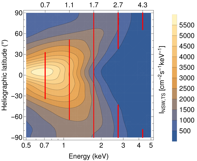
Independently of the charge exchange, the fluxes of the supersonic solar wind and the already created NSW decrease with distance, thus at the termination shock they need to be multiplied by the squared ratio of distances at 1 AU () and at the termination shock (): . The charge exchange process that is the source of the NSW is also responsible for the exponential decrease of the solar wind proton flux (). The bulk speed is decreasing according to Equation (1). We smooth the NSW speed distribution using the normal (Gaussian) distribution with the mean value equal to the speed at the considered distance and the standard deviation km s-1 equal to the spread of the model speeds from Sokół et al. (2015) and these observed by in-ecliptic spacecraft, collected in the OMNI database. We do so because in situ observations show that the velocity distribution function of the solar wind accumulated over the intervals of CR are much wider than it would be implied by the purely thermal spread of proton velocities. Figure 1 presents the differential flux NSW given by Equation (4) as a function of energy and heliographic latitude.
2.2 Analytic model of secondary ENA emission
In this analysis, we use an analytic model of the ribbon generation by the secondary ENA mechanism based on the observational constraints on the position and width of the ribbon in the sky. The model is an extension of the model by Möbius et al. (2013). We employ the version of the model previously used in the assessment of the expected secondary helium ENA emission by Swaczyna et al. (2014). With some rearrangement, the formula for the ENA differential intensity at IBEX can be expressed as:
| (5) |
where
| (6) |
This form consists of three factors: the geometric factor , the NSW flux at the termination shock , and the dimensionless factor that accounts for the ionization and re-neutralization of the NSW, with the inverse-square law for the NSW flux included. Below, we describe the necessary modification of this formula in our analysis.
In the original form it was assumed that the NSW flux is monoenergetic, so the flux was presented as a simple product of the density and speed of the NSW. The total flux was assumed to fit into a single IBEX energy channel with the width . Here, we replace this term with the differential NSW flux at the termination shock , which depends on the energy and heliographic latitude .
The factor represents the effective part of the NSW that forms the secondary ENA. It is normalized to the flux of the solar wind at the termination shock. This is a convenient choice because the accumulation of the NSW ceases at the termination shock. In the formula and represent the distances to the termination shock and to the heliopause, respectively. The integrals run over , which denotes the distance of the ionization of the primary ENA, and , which denotes the distance where the re-neutralization occurs. The termination shock distance is assumed to be omni-directionally constant and equal to 90 AU, i.e., in the middle of the two distances of the termination shock crossing by Voyager 1 and Voyager 2 at 94 AU and 84 AU, respectively (Burlaga et al., 2005; Gurnett & Kurth, 2005; Burlaga et al., 2008; Gurnett & Kurth, 2008). For the heliopause distance we use a simple axisymmetrical model of the heliosphere with incompressible plasma flow by Suess & Nervey (1990), for which we select the parameters so that the termination shock distance is 90 AU, and the distance to the heliopause at the Voyager 1 direction is 121 AU, as observed (Gurnett et al., 2013). With this model, the distance to the heliopause at the directions along the ribbon changes in the range 120–200 AU. The model used for the heliopause distance does not contain magnetic field and does not reconstruct the observed two-lobed structure of the heliotail (McComas et al., 2013). One of these lobes is coincident with the natural continuation of the ribbon location, and the ribbon signal is suppressed in this part of the sky. This effect is not reproduced by our model, but we drop this part of the ribbon from the analysis for the reasons described below. Finally, the heliopause distance is solely a function of the angular distance to the heliospheric nose, denoted as , i.e., it is assumed to feature axial symmetry around the inflow direction.
The mean free path for ionization of ENAs in the LISM and the effective mean free path for neutralization of the pick-up protons in the LISM depend on the considered energy and are given by the following formulae:
| (7) | ||||
| (8) |
where and are cross sections for the charge exchange between hydrogen atom and protons (Lindsay & Stebbings, 2005) and for the ionization of hydrogen atom by impact of another hydrogen atom (Barnett, 1990), respectively. The quantities and are the densities of protons and hydrogen atoms in the LISM (Frisch et al., 2011). The effective mean free path for protons also depends on The resulting value of the factor is presented in Figure 2. This factor has values in the range of 2.5–6% with these assumptions, and moderately depends on the energy.

The geometric factor defines the solid angle into which the secondary ENAs are emitted. This factor effectively reflects the draping of the interstellar magnetic field and the creation and stability of the ring distribution of the pick-up primary ENAs that gyrate around the draped magnetic field line before re-neutralization. Using effective geometric factor is justified since it was found that the magnetic field draping alone cannot explain the energy dependence of the ribbon position (Zirnstein et al., 2016a). Originally, the model assumed that the pick-up ions form a narrow cold ring distribution, such that the produced ENA fit entirely into the IBEX field of view with the FWHM of (Möbius et al., 2013). However, from the separation of the ribbon from the generally distributed flux it was found that the ribbon is broader (Schwadron et al., 2011, 2014). Thus, we replace the formula presented in Equation (5) with the following one:
| (9) |
where is the standard width of the ribbon, which we adopt to reproduce the observed ribbon FWHM of 25° (Schwadron et al., 2014). We assume that the geometric factor depends only on the distance to the ribbon center at ecliptic , with a maximum at the distance (Funsten et al., 2013). We constructed this factor so that it does not depend on energy. Therefore, we adopt the parameters of the ribbon position obtained from averaging over energy channels. Consequently, the obtained shift of the fitted centers must be caused by the two others factors in Equation (5).
Finally, the intensity of the secondary ENA for energy in direction can be expressed as a product of three factors:
| (10) |
where is the geometric factor given by Equation (9), is the NSW flux, given by Equation (4), and is the reflectance factor, defined as in Equation (6).
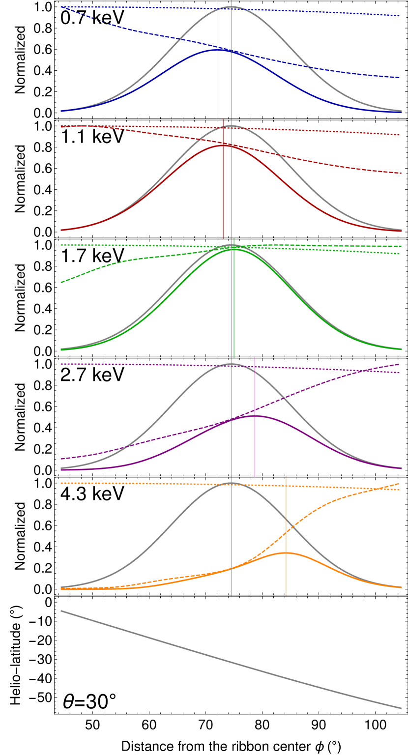
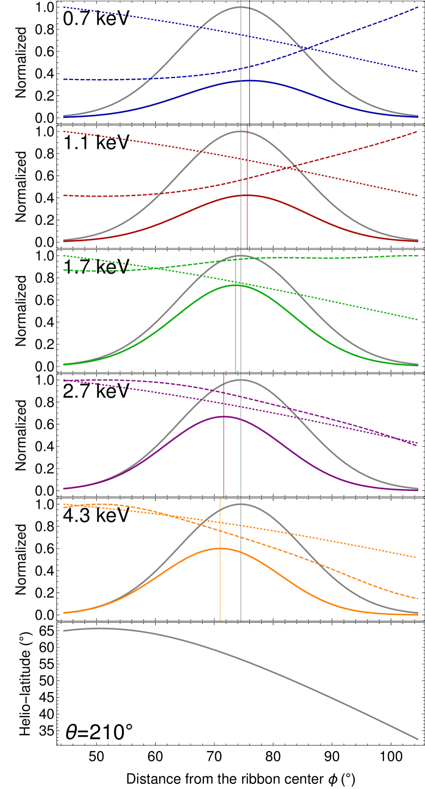
2.3 Mechanism of the ribbon shift
2.4 Fitting of circles and ellipses
We the ENA intensity over the sky using the model of the secondary ENA emission presented above. Below, we describe the procedure used to find the circular and elliptic fits to the locations of the maximal signal along the ribbon. The procedure was tuned to follow the idea used previously by Funsten et al. (2013) to obtain the fits to the data.
We integrate the signal given by Equation (10) over the bins in the ribbon coordinates and over energies with the IBEX-Hi energetic response function (Funsten et al., 2009a) for the respective energy channel. The same pixelization scheme was previously used in the data analysis by Funsten et al. (2013). It is a different scheme from the scheme typically used to present IBEX data, where the basis is the ecliptic coordinate system (McComas et al., 2014b). Subsequently, for each of the 60 meridian profiles we select 7 pixels so that the center pixel has the highest signal. The selected range of pixels is fitted to the Gaussian shape given by the formula: . The fitted peak positions do not contain the uncertainties resulting from the statistical scatter, which is the main contributor to the total uncertainty in the analysis of the observations (Funsten et al., 2013).
The fitted shapes (circles and ellipses) are not expected to reproduce the ribbon precisely. They are intended to be alternative, simplified descriptions of the ribbon morphology. In other words, we do not expect that with higher statistics, the location of the maximum signal of the ribbon will approach the position encircled by the fitted circle or ellipse. Consequently, we follow the selection of the pixels used in the original data analysis by Funsten et al. (2013), and we need to weight the pixels to acknowledge the relative uncertainties of the fits to the data.
Based on this prerequisite, we minimize the and estimators for the circular and elliptic models in the forms:
| (11) | |||
| (12) |
where s represent the directions in the sky in whichever coordinate system, and returns the angular distance between the directions. The summation is over the ribbon positions in the azimuthal sectors enumerated by , which run over the same sectors as those used in the data fitting by Funsten et al. (2013). The quantities represent the heights of the ribbon profile, which we use for weighting.
In the case of the circular fit, the parameters are the position of the ribbon center and the ribbon radius . In the case of the elliptic fit, the parameters are the directions of the ellipse foci , and the semi-major axis . Equivalently, the ellipse can be described by the following set of parameters: the center direction , the semi-major axis , the semi-minor axis , and the rotation angle . We also derive the eccentricity . We transform the fitted parameters to this set, since it was used for the data analysis by Funsten et al. (2013). The rotation angle is given in the ribbon coordinates.
3 Results and discussion
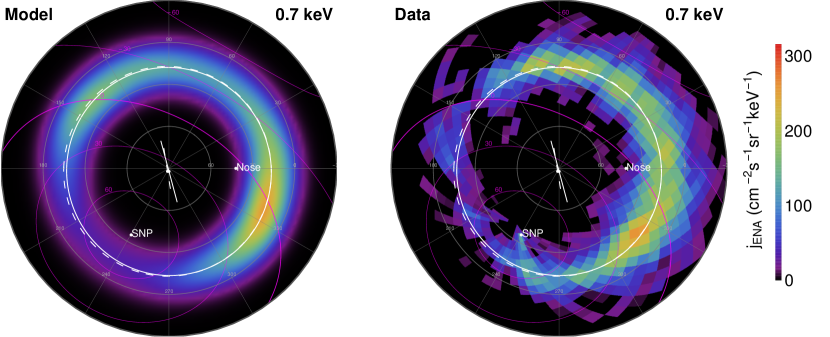
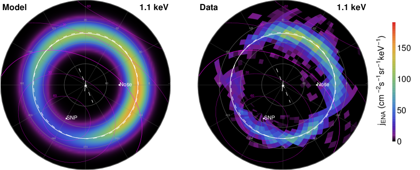
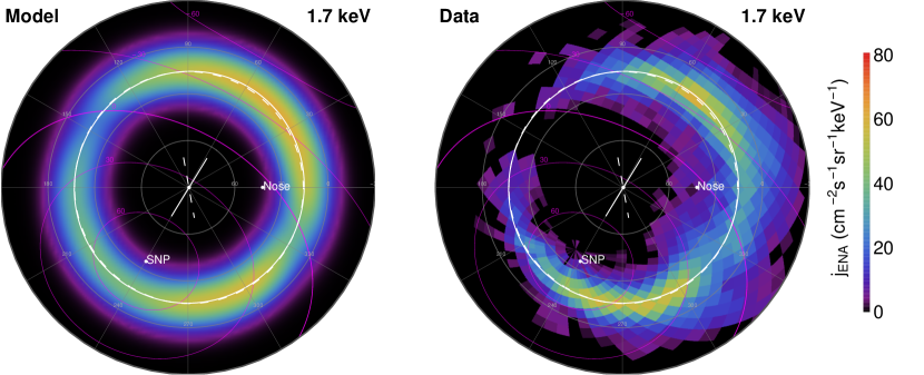
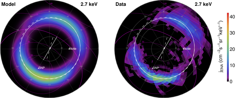
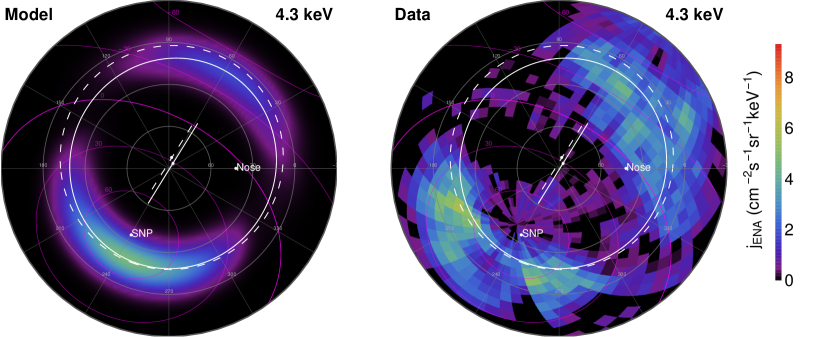
The is compared with the signal extracted from the observations by Schwadron et al. (2014)222The numerical values of ribbon signal extracted from the data are available as IBEX Data Release 8 Schwadron et al. (2014) at http://ibex.swri.edu/ibexpublicdata/Data_Release_8. in Figures 4 & 5. The maps are plotted in the ribbon coordinates, so they can be compared also with the maps in the previous analysis by Funsten et al. (2013, Figures 2 & 3). In Table 1 we compare these parameters obtained from our fitting and the one found by Funsten et al. (2013) from data analysis. The mean deviations between the ribbon locations and the fitted ellipses and circles are denoted as and , respectively.
| Elliptic fit | Circular fit | |||||||||||
|---|---|---|---|---|---|---|---|---|---|---|---|---|
| (keV) | (°) | (°) | (°) | (°) | (°) | (°) | (°) | (°) | (°) | (°) | ||
| 0.7 | daa‘d’ denotes the parameters from the fitting to the data obtained by Funsten et al. (2013), and (this analysis). | 219.8 | 42.2 | 97.4 | 74.9 | 73.2 | 0.22 | 1.4 | 218.5 | 43.1 | 74.8 | 2.1 |
| m | 221.0 | 41.7 | 103.0 | 74.4 | 71.0 | 0.30 | 0.3 | 220.2 | 42.5 | 74.3 | 0.3 | |
| 1.1 | d | 220.6 | 40.2 | 111.3 | 75.4 | 71.0 | 0.34 | 1.8 | 220.3 | 40.5 | 73.3 | 2.4 |
| m | 219.9 | 41.3 | 83.5 | 74.4 | 74.0 | 0.09 | 0.3 | 219.9 | 41.3 | 74.3 | 0.3 | |
| 1.7 | d | 219.9 | 39.7 | 100.0 | 74.4 | 71.8 | 0.26 | 1.5 | 219.6 | 39.8 | 73.2 | 1.7 |
| m | 219.9 | 39.4 | 58.5 | 74.7 | 71.5 | 0.29 | 0.6 | 219.4 | 39.4 | 74.4 | 0.7 | |
| 2.7 | d | 218.8 | 37.6 | 76.3 | 75.7 | 70.9 | 0.35 | 1.8 | 217.9 | 37.7 | 74.4 | 2.2 |
| m | 219.9 | 37.6 | 60.8 | 75.3 | 67.8 | 0.43 | 0.5 | 218.9 | 37.6 | 74.8 | 0.8 | |
| 4.3 | d | 215.5 | 32.5 | 65.3 | 80.3 | 75.7 | 0.33 | 2.9 | 214.2 | 32.4 | 79.2 | 3.0 |
| m | 219.5 | 35.4 | 61.6 | 75.9 | 68.2 | 0.44 | 0.8 | 218.6 | 35.4 | 75.5 | 1.0 | |
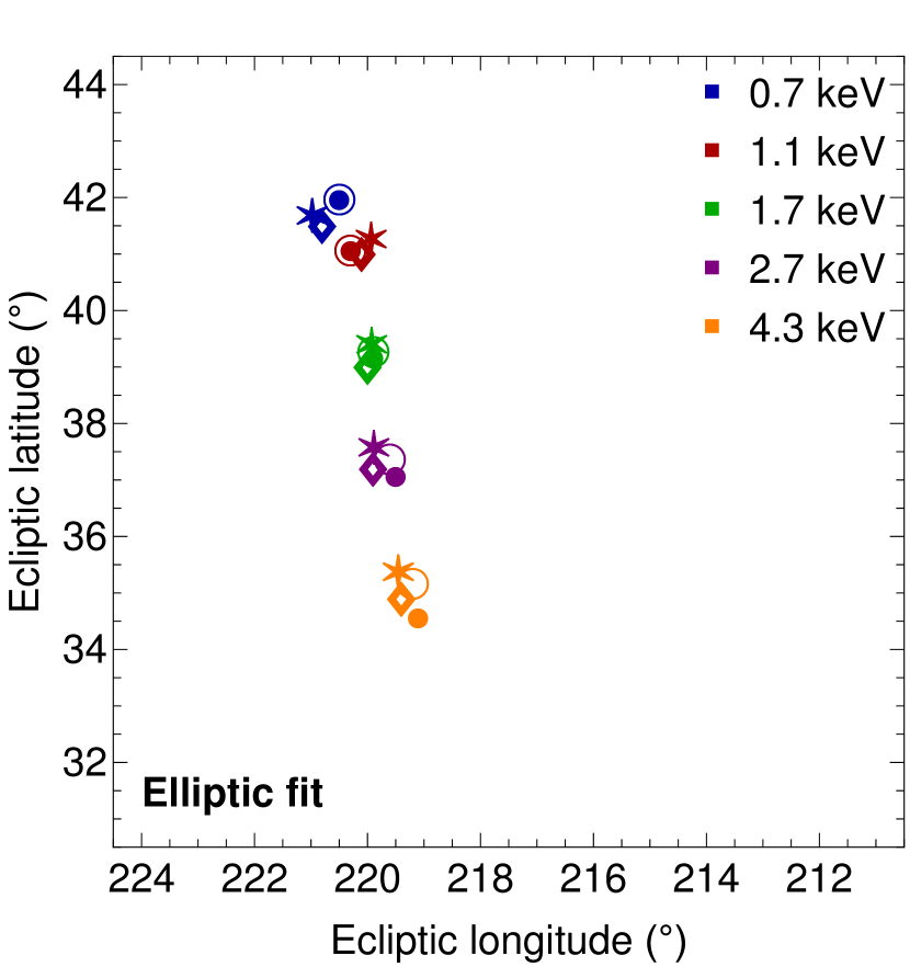
We compare the fitted centers in Figure 6. The displacements of the fit centers between subsequent energy channels obtained from the match those obtained by Funsten et al. (2013) from the data analysis. The energy sequence is not aligned along the plane that includes the interstellar neutral flows and the ribbon center (Kubiak et al., 2016), known as the neutral deflection plane (black line in Figure 6), but it is approximately parallel to Such a procedure probably overestimated the actual uncertainties. Consequently, we are not able to formally check the consistency between the data and results. The ellipticities expressed by the rotation angle and eccentricities are similar for the observations and , even though we have assumed a simple circular shape for the geometric factor.
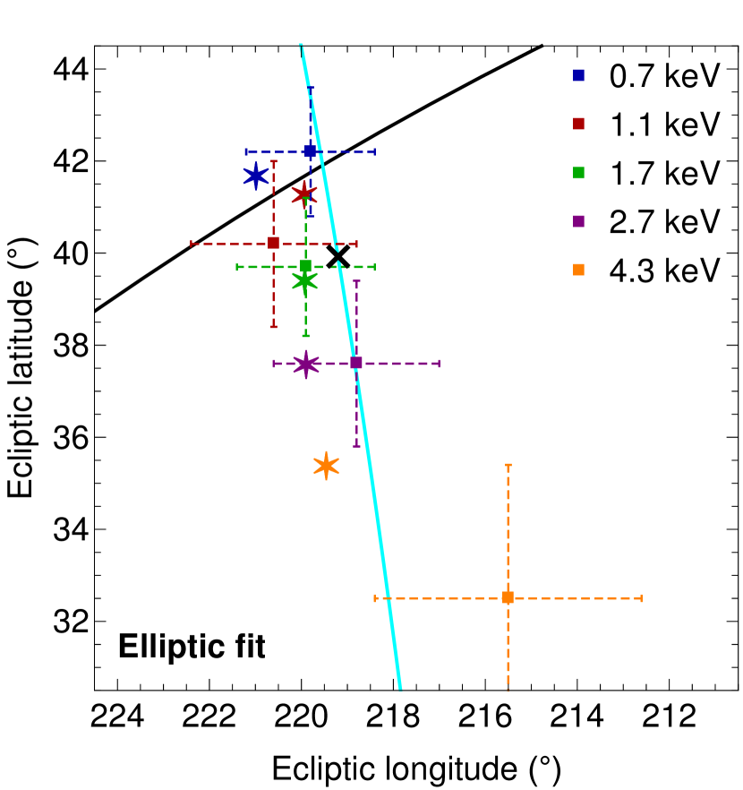
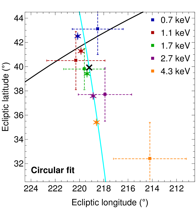
The circular fits are intended as a sanity test for our baseline results, obtained from the elliptic fits: a qualitative difference between the two models would cast doubt on the credibility of our conclusions. But the results from the circular fits are similar to the elliptic fits. In the case of circular fits, the centers are even better aligned with the local heliographic meridian. Comparing the mean differences of the peak location to the fitted signal ( vs ), it is visible that elliptic fits are better. This is a natural consequence, since the ellipse is generalization of the circle.
we conclude that our results and conclusions on the role of the solar wind structure in shaping the position of the ribbon are robust.
The largest discrepancy occurs for the highest energy channel. In the , the centers for the consecutive energy channels are shifted by the same magnitude for all energy channels, but in the data the highest energy channel is shifted the most, and also the ribbon radius increases accordingly, which is not observed in the . Another discrepancy is in the fit for the energy 1.7 keV, which in the elliptic case agrees well in all aspects except for the rotation angle (58° for the fit and 100° for the data fit). Most of the deviations arise due to the statistical dispersion in the data, since the deviations of the ribbon location from the fitted shape () are 4-fold larger in the data than in the . The non-vanishing values of for the suggest that the model of a circular or elliptic shape is too simple to adequately describe the ribbon.
The presented simple model of the secondary ENA mechanism with helio-latitudinal structure of the solar wind reproduces the effect of the energy dependence of the fitted centers of the IBEX ribbon very well for most of the IBEX energy channels. The discrepancy in the highest energy channel could suggest that for the highest energy at least a portion of the signal may be due to a different mechanism of the ENA generation. An argument in favor of this hypothesis is that the ENA intensities obtained from INCA on board the Cassini spacecraft for energies higher than at IBEX reveals a similar feature as the ribbon, called the INCA belt (Krimigis et al., 2009; Dialynas et al., 2013), but the center of the belt at is shifted much farther than the IBEX ribbon center. However, the energies of ENAs observed by INCA are well above the energies typical for the solar wind, and thus the belt is not likely explained as the reflectance of the NSW.
The helio-latitudinal structure of the supersonic solar wind was previously included in several analyses (Heerikhuisen et al., 2014; Zirnstein et al., 2015, 2016b). However, these analyses did not report any findings concerning the effect of energy-dependent shift of the ribbon center (Zirnstein et al., 2015, 2016b), or such an effect was not visible (Heerikhuisen et al., 2014).
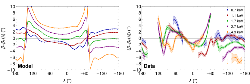
As a by-product of the analysis of the ribbon parallax, Swaczyna et al. (2016) obtained deviations of the locations of the maximum signal of the ribbon in the ecliptic coordinates from the positions expected from a circle centered at with the radius . In Figure 8 we compare those results with the deviations obtained in our analysis. In the figure we do not use the fitted shapes, but the actual positions of the maximum signal obtained as the intermediate step in the fitting procedure. The results cover almost the whole sky, because we can fit the position for any signal level, whereas when fitting the data one needs to adopt a certain threshold value for the signal to noise ratio to find a meaningful fit.
In the case of a perfectly adequate model the respective lines from the should fit to the data uncertainty bands, but our model is far too simple to expect a perfect fit. We notice, however, that the energy sequence for the ecliptic longitudes is the same in the data and in the . Also the discontinuities for ecliptic longitudes 75° and –140° are visible both in the data and in the . These discontinuities coincide with the intersection of the heliographic equator by the ribbon locations. These results additionally support the connection between the NSW and the IBEX Ribbon.
4 Summary and conclusions
In this analysis we extended the analytical model of the secondary ENA emission originally proposed by Möbius et al. (2013), which we supplemented with the model of the primary ENAs produced in the helio-latitudinally structured supersonic solar wind. The primary ENAs are created by charge-exchange of the solar wind inside the termination shock with the neutral background atoms. The solar wind was modeled using the helio-latitudinal structure from the model by Sokół et al. (2015). The distribution of the primary ENAs was built for each CR separately and next averaged over Solar Cycle 23. The obtained signals were subsequently fitted to the circles and ellipses, as was done in the analysis of the IBEX data by Funsten et al. (2013). The fitted parameters, including the centers of the circles and ellipses, were compared between the data and .
The ribbon centers for the IBEX-Hi energy channels form a monotonic sequence that is well aligned with the . The obtained magnitude of this effect is similar to that observed in the data, except for the highest IBEX-Hi energy channel, for which the shift between the two highest channels in the data is much larger than for the other pairs of the consecutive channels, what is not observed in the . This, together with observations of the INCA belt, suggest that in addition to the secondary ENA mechanism that forms the ribbon, a different mechanism may be operating in the vicinity of the heliosphere, responsible for a part of the ENA signal in the highest IBEX energy channels and for the INCA belt.
With the presented model, we reproduced two important features of the ribbon structure: the evolution in the relative magnitude of the signal along the ribbon and the shift of the ribbon center with increasing energy. The first effect was already understood in previous analyses (McComas et al., 2014b), but the latter one is explained for the first time. Our findings explain these important features of the ribbon as closely related to each other and strongly support the mechanism of the secondary ENA emission with the interstellar magnetic field lines draped in the outer heliosheath as the most likely mechanism of the ribbon generation. This finding is additionally supported by the distance to the ribbon, determined to be at about 140 AU (Swaczyna et al., 2016). We thus showed that details of the ribbon depend as much on the processes operating in the outer heliosheath as on the details of the solar wind structure and its evolution during the solar cycle.
References
- Barnett (1990) Barnett, C. F. 1990, Atomic Data for Fusion, Vol. 1, Collisions of H, H2, He and Li atoms and ions with atoms and molecules (Oak Ridge National Laboratory)
- Burlaga et al. (2008) Burlaga, L. F., Ness, N. F., Acuña, M. H., et al. 2008, Natur, 454, 75
- Burlaga et al. (2005) —. 2005, Sci, 309, 2027
- Bzowski et al. (2008) Bzowski, M., Möbius, E., Tarnopolski, S., Izmodenov, V., & Gloeckler, G. 2008, SSRv, 143, 177
- Bzowski et al. (2013a) Bzowski, M., Sokół, J. M., Kubiak, M. A., & Kucharek, H. 2013a, A&A, 557, A50
- Bzowski et al. (2001) Bzowski, M., Summanen, T., Ruciński, D., & Kyrölä, E. 2001, The Outer Heliosphere: The Next Frontiers: The Next Frontiers, 11
- Bzowski et al. (2013b) Bzowski, M., Sokół, J. M., Tokumaru, M., et al. 2013b, in Cross-Calibration of Far UV Spectra of Solar System Objects and the Heliosphere, ed. E. Quémerais, M. Snow, & R.-M. Bonnet, ISSI Scientific Report Series No. 13 (Springer New York), 67–138
- Bzowski et al. (2015) Bzowski, M., Swaczyna, P., Kubiak, M. A., et al. 2015, ApJS, 220, 28
- Coles et al. (1980) Coles, W. A., Rickett, B. J., Rumsey, V. H., et al. 1980, Natur, 286, 239
- Dialynas et al. (2013) Dialynas, K., Krimigis, S. M., Mitchell, D. G., Roelof, E. C., & Decker, R. B. 2013, ApJ, 778, 40
- Fahr & Ruciński (2001) Fahr, H. J., & Ruciński, D. 2001, in The 3-D Heliosphere at Solar Maximum, ed. R. G. Marsden (Springer Netherlands), 407–412
- Fahr & Ruciński (2002) —. 2002, NPGeo, 9, 377
- Frisch et al. (2011) Frisch, P. C., Redfield, S., & Slavin, J. D. 2011, ARA&A, 49, 237
- Funsten et al. (2009a) Funsten, H. O., Allegrini, F., Bochsler, P., et al. 2009a, SSRv, 146, 75
- Funsten et al. (2009b) Funsten, H. O., Allegrini, F., Crew, G. B., et al. 2009b, Sci, 326, 964
- Funsten et al. (2013) Funsten, H. O., DeMajistre, R., Frisch, P. C., et al. 2013, ApJ, 776, 30
- Funsten et al. (2015) Funsten, H. O., Bzowski, M., Cai, D. M., et al. 2015, ApJ, 799, 68
- Fuselier et al. (2009) Fuselier, S. A., Allegrini, F., Funsten, H. O., et al. 2009, Sci, 326, 962
- Gloeckler et al. (2004) Gloeckler, G., Möbius, E., Geiss, J., et al. 2004, A&A, 426, 845
- Gurnett & Kurth (2005) Gurnett, D. A., & Kurth, W. S. 2005, Sci, 309, 2025
- Gurnett & Kurth (2008) —. 2008, Natur, 454, 78
- Gurnett et al. (2013) Gurnett, D. A., Kurth, W. S., Burlaga, L. F., & Ness, N. F. 2013, Sci, 341, 1489
- Heerikhuisen et al. (2006) Heerikhuisen, J., Florinski, V., & Zank, G. P. 2006, JGRA, 111, A06110
- Heerikhuisen et al. (2014) Heerikhuisen, J., Zirnstein, E. J., Funsten, H. O., Pogorelov, N. V., & Zank, G. P. 2014, ApJ, 784, 73
- Heerikhuisen et al. (2010) Heerikhuisen, J., Pogorelov, N. V., Zank, G. P., et al. 2010, ApJL, 708, L126
- Isenberg (2014) Isenberg, P. A. 2014, ApJ, 787, 76
- Izmodenov et al. (2013) Izmodenov, V. V., Katushkina, O. A., Quémerais, E., & Bzowski, M. 2013, in ISSI Scientific Report Series, Vol. 13, Cross-Calibration of Far UV Spectra of Solar System Objects and the Heliosphere (New York: Springer Science+Business Media), 7
- Kakinuma (1977) Kakinuma, T. 1977, in Astrophysics and Space Science Library, Vol. 71, Study of Travelling Interplanetary Phenomena, ed. M. A. Shea, D. F. Smart, & S. T. Wu, 101–118
- King & Papitashvili (2005) King, J. H., & Papitashvili, N. E. 2005, JGRA, 110, A02104
- Krimigis et al. (2009) Krimigis, S. M., Mitchell, D. G., Roelof, E. C., Hsieh, K. C., & McComas, D. J. 2009, Sci, 326, 971
- Kubiak et al. (2016) Kubiak, M. A., Swaczyna, P., Bzowski, M., et al. 2016, ApJS, 223, 25
- Lee et al. (2009) Lee, M. A., Fahr, H. J., Kucharek, H., et al. 2009, SSRv, 146, 275
- Lindsay & Stebbings (2005) Lindsay, B. G., & Stebbings, R. F. 2005, JGRA, 110, A12213
- McComas et al. (2013) McComas, D. J., Dayeh, M. A., Funsten, H. O., Livadiotis, G., & Schwadron, N. A. 2013, ApJ, 771, 77
- McComas et al. (2008) McComas, D. J., Ebert, R. W., Elliott, H. A., et al. 2008, GeoRL, 35, L18103
- McComas et al. (2014a) McComas, D. J., Lewis, W. S., & Schwadron, N. A. 2014a, RvGeo, 52, 2013RG000438
- McComas et al. (2009a) McComas, D. J., Allegrini, F., Bochsler, P., et al. 2009a, Sci, 326, 959
- McComas et al. (2009b) —. 2009b, SSRv, 146, 11
- McComas et al. (2012) McComas, D. J., Dayeh, M. A., Allegrini, F., et al. 2012, ApJS, 203, 1
- McComas et al. (2014b) McComas, D. J., Allegrini, F., Bzowski, M., et al. 2014b, ApJS, 213, 20
- Möbius et al. (2013) Möbius, E., Liu, K., Funsten, H., Gary, S. P., & Winske, D. 2013, ApJ, 766, 129
- Parker (1958) Parker, E. N. 1958, ApJ, 128, 664
- Parker (1961) —. 1961, ApJ, 134, 20
- Phillips et al. (1995) Phillips, J. L., Bame, S. J., Barnes, A., et al. 1995, GeoRL, 22, 3301
- Pogorelov et al. (2009) Pogorelov, N. V., Heerikhuisen, J., Zank, G. P., Mitchell, J. J., & Cairns, I. H. 2009, AdSpR, 44, 1337
- Richardson et al. (2008) Richardson, J. D., Liu, Y., Wang, C., & McComas, D. J. 2008, A&A, 491, 1
- Schwadron & McComas (2013) Schwadron, N. A., & McComas, D. J. 2013, ApJ, 764, 92
- Schwadron et al. (2009) Schwadron, N. A., Bzowski, M., Crew, G. B., et al. 2009, Sci, 326, 966
- Schwadron et al. (2011) Schwadron, N. A., Allegrini, F., Bzowski, M., et al. 2011, ApJ, 731, 56
- Schwadron et al. (2014) Schwadron, N. A., Moebius, E., Fuselier, S. A., et al. 2014, ApJS, 215, 13
- Sokół et al. (2013) Sokół, J. M., Bzowski, M., Tokumaru, M., Fujiki, K., & McComas, D. J. 2013, SoPh, 285, 167
- Sokół et al. (2015) Sokół, J. M., Swaczyna, P., Bzowski, M., & Tokumaru, M. 2015, SoPh, 290, 2589
- Suess & Nervey (1990) Suess, S. T., & Nervey, S. 1990, JGRA, 95, 6403
- Swaczyna et al. (2016) Swaczyna, P., Bzowski, M., Christian, E. R., et al. 2016, ApJ, 823, 119
- Swaczyna et al. (2014) Swaczyna, P., Grzedzielski, S., & Bzowski, M. 2014, ApJ, 782, 106
- Tarnopolski & Bzowski (2009) Tarnopolski, S., & Bzowski, M. 2009, A&A, 493, 207
- Tokumaru et al. (2010) Tokumaru, M., Kojima, M., & Fujiki, K. 2010, JGRA, 115, A04102
- Zirnstein et al. (2016a) Zirnstein, E. J., Funsten, H. O., Heerikhuisen, J., & McComas, D. J. 2016a, A&A, 586, A31
- Zirnstein et al. (2016b) Zirnstein, E. J., Heerikhuisen, J., Funsten, H. O., et al. 2016b, ApJL, 818, L18
- Zirnstein et al. (2015) Zirnstein, E. J., Heerikhuisen, J., Pogorelov, N. V., McComas, D. J., & Dayeh, M. A. 2015, ApJ, 804, 5