Generalized Centripetal Force Law and Quantization of Motion Constrained on $2D$ Surfaces

Abstract

For a particle moves on a $2D$ surface $f(\mathbf{x})=0$ embedded in $3D$ Euclidean space, the geometric momentum and potential are simultaneously admissible within the Dirac canonical quantization scheme for constrained motion. In our approach, not the full scheme but the symmetries indicated by classical brackets $[x,H]_{D}$ and $[p,H]_{D}$ in addition to the fundamental ones $[\mathbf{x},\mathbf{x}]_{D}$, $[\mathbf{x},\mathbf{p}]_{D}$ and $[\mathbf{p},\mathbf{p}]_{D}$ are utilized, where the subscript $D$ stands for the Dirac bracket. The generalized centripetal force law $\mathbf{\dot{p}=}[\mathbf{p},H]_{D}$ for particle on the $2D$ surface play the key role, and there is no simple relationship between the force on a point of the surface and its curvatures of the point, in sharp contrast to the motion on a curve.

Introduction For the motion constrained on a $2D$ surface $\Sigma\subseteq E^{3}$ described by an implicit equation $f(\mathbf{x})=0$ where $\mathbf{x}$ are the usual Cartesian coordinates, there are extrinsic-curvature dependent geometric momentum and potential, jk ; dacosta ; FC ; liu11-1 ; liu13-1  resulting from the so-called confining technique. By the confining technique, the surface is not a mathematically surface without thickness but a $3D$ object in $E^{3}$ with e.g. thickness of at least one atom, thus we can first imagine that there is a confining potential crossing the surface, e.g., a harmonic potential $\mu\omega^{2}b^{2}/2$ with $\mu$ denoting the mass and $b$ being the normal coordinate of the surface, then let the confining strength $\omega$ be so larger that the motion constrained on the surface $f(\mathbf{x})=0$ is realized. The resultant geometric potential was recently experimentally confirmed. exp1 ; exp2 However, there is a difficulty: if we start the surface equation $f(\mathbf{x})=0$ and work within the formalism of Dirac’s theory of constrained systems, dirac1 ; dirac2 the desired form of the geometric potential appears to be unattainable. homma ; ikegami ; matsutani ; Kleinert The known resolution was to resort to another but derived form of constraint $df(\mathbf{x})/dt=0$ with the consistent form of the classical Hamiltonian which differs from the usual one $H_{c}=\mathbf{p}^{2}/2\mu$, even for simplicity only the kinetic energy is considered. Homma group and Ikegami group have independently developed a formalism that opens a wide door to various forms of the curvature-induced potentials that contain the geometric one as a special case. homma ; ikegami Furthermore, Matsutani examined both the classical and quantum mechanics for motion constrained on the $2D$ surfaces, and concluded that the constraint $f(\mathbf{x})=0$ is not physical at all. matsutani However, during recent years, we dealt with some $2D$ surfaces, case-by-case, and found that the constraint $f(\mathbf{x})=0$ is truly physical as well, if not more. liu11-1 ; liu13-3 ; liu14-1 In the present work, we report a universal way to resolve the problem.

There is a working hypothesis that Hamiltonian operator for a system on $2D$ surfaces also takes the usual form $H=\mathbf{p}^{2}/2\mu$ with proper form of the momenta $\mathbf{p=(}p_{x},p_{y},p_{z}\mathbf{)}$, and it is unfortunately too much widely accepted. homma ; ikegami ; matsutani ; Kleinert ; weinberg In flat space this hypothesis works, because it is nothing but a consequence of the full Dirac canonical quantization scheme, dirac3 which formally states that all symmetries expressed by the Poisson brackets $[\alpha,\beta]_{P}$ between any pair of two classical quantities $\alpha$ and $\beta$ persist in quantum mechanics. dirac1 ; dirac2 ; dirac3 So, once the working hypothesis meets with difficulty or fails, we have to turn to the fundamental principles. In order to get the quantum Hamiltonian without invoking the the full Dirac canonical quantization scheme, we should require that $[\mathbf{x},H_{c}]_{D}$ and $[\mathbf{p},H_{c}]_{D}$, where $[\alpha,\beta]_{D}$ denotes that Dirac bracket, persist in quantum mechanics. This is the minimum enlargement of the quantization rule from the fundamental ones among $\mathbf{x}$ and $\mathbf{p}$, i.e., $\left[\mathbf{x,x}\right]$, $\left[\mathbf{x,p}\right]$ and $\left[\mathbf{p,p}\right]$ to include $[\mathbf{x},H]$ and $[\mathbf{p},H]$. The Hamiltonian operator is simultaneously determined by commutation relations and $[\mathbf{x,}H]\equiv i\hbar O\left([\mathbf{x},H_{c}]_{D}\right)$ and $[\mathbf{p,}H]\equiv i\hbar O\left([\mathbf{p},H_{c}]_{D}\right)$, provided that there is classical Hamiltonian $H_{c}$, where $O\left(\alpha\right)$ is the proper form of the quantum operator representing the classical quantity $\alpha$. This is the so-called an enlarged canonical quantization scheme for the constrained motion on the hypersurface. liu11-1 ; liu13-2 ; liu15 ; note This scheme leads to the quantum Hamiltonian $H=\mathbf{p}^{2}/2\mu$ for the free motion in flat space. In addition, it leads to the geometric momentum ${\mathbf{p}}=-i\hbar({\nabla_{\Sigma}}+{M{\mathbf{n/}}}2)$ liu13-2 ; note1 where ${\nabla_{\Sigma}}$ is the gradient operator defined on the hypersurface, and ${{\mathbf{n}}}$ is the unit normal vector, and the mean curvature ${M}$ is usually defined by the sum of all principal curvatures on the hypersurface. But for a $2D$ surface, the mean curvature is usually defined by the true average so we use ${\mathbf{p}}=-i\hbar({\nabla_{\Sigma}}+{M{\mathbf{n}}})$ in the rest part of the Letter.

In whole of this study, we consider the free motion only without involving the external forces which can be simply treated if no coupling between the external forces and the curvature of the surface. After quantization, the quantum free motion Hamiltonian on the surface has curvature-induced geometric momentum potential $V_{g}\equiv-\mathbf{\hbar}^{2}\left(M^{2}-K\right)/(2\mu)$, jk ; dacosta ; FC ; liu11-1 ; liu13-1

$$H_{c}=\frac{\mathbf{p}^{2}}{2\mu}\rightarrow H=-\frac{\mathbf{\hbar}^{2}}{2\mu}\Delta_{LB}+V_{g}=-\frac{\mathbf{\hbar}^{2}}{2\mu}\left(\Delta_{LB}+M^{2}-K\right)$$ (1)

where $\Delta_{LB}$ is the Laplace-Betrami operator on the surface, and $K$ is the Gaussian curvature and it is zero for the cylinder, cone, etc..

For the particle moving on the $2D$ surface $f(\mathbf{x})=0$, the unit normal vector is $\mathbf{n=}\nabla f/\left|\nabla f\right|$. In classical mechanics, we have for the time derivative $\mathbf{\dot{p}\equiv}d\mathbf{p}/dt$ of momentum $\mathbf{p}$, ikegami ; weinberg ; note2

$$\mathbf{\dot{p}=-np\cdot\nabla n\cdot p/}\mu.$$ (2)

It in fact expresses the generalized centripetal force law (GCFL) which should reduce to the usual one $a=v^{2}/R$ as the particle is constrained on a curve, so this relation must then be in general expressible as those between kinematic quantities and intrinsic/extrinsic curvatures. With noting $\mathbf{\dot{p}=}\left[\mathbf{p,}H_{c}\right]_{D}$, the enlarged canonical quantization scheme implies that the following relation holds true during quantization,

$$\left[\mathbf{p,}H\right]=-i\hbar O\left(\mathbf{np\cdot\nabla n\cdot p/}\mu\right),$$ (3)

The key finding of this Letter is that the geometric momentum and potential can automatically appear in this relation (3). We will first deal with some special $2D$ surfaces then make remarks on the general one.

Case 1: motion on cylinders By the $2D$ cylinder we mean a ruled surface spanned by a one-parameter family of parallel lines along $z$-axis for convenience. So the cross section of the cylinder can be an ellipse, a parabola, a hyperbola, and a curved or even a straight line, and their equations can be assumed to be given by $y=u(x)$ whose curvatures take the form $\kappa=$ $1/R=u^{\prime\prime}(x)/(1+u^{\prime}(x)^{2})^{3/2}$. It is easily understandable that GCFL (2) takes the following form for it is nothing but another form of well-known one $a=v^{2}/R$,

$$\mathbf{\dot{p}}=-4\mathbf{M}H_{c}=2H_{c}\mathbf{n}/R,\text{ or, }\left[\mathbf{p,}H_{c}\right]_{D}=2H_{c}\mathbf{n}/R,$$ (4)

where $H_{c}=\mu v^{2}/2=\left(p_{x}^{2}+p_{y}^{2}\right)/2\mu$ is the classical Hamiltonian for the motion on the the cross section for the motion along axis of the cylinder is trivial thus is neglected, $\mathbf{M=-n}/\left(2R\right)$ is the mean curvature vector, a geometric invariant, and $\mathbf{n}$ being the normal vector. To note that, in differential geometry, mean curvature is defined by $M=-1/\left(2R\right)$ whose sign depends on the choice of normal, negative if the normal points along the convex side of the surface. Equation (4) shows that the generalized centripetral force is proportional to the mean curvature.

In quantum mechanics, Eq. (3) is now,

$$\left[\mathbf{p,}H\right]=i\hbar O\left(2H_{c}\mathbf{n}/R\right).$$ (5)

Previous studies demonstrate that no matter what form of the momentum is taken, the Hamiltonian operator $H=\mathbf{p}^{2}/2\mu$ is not able to include the geometric potential. homma ; ikegami ; matsutani Instead, it is an easy task to establish the following equations for unknown functions $q_{i}(x)$ ($i=x,y$),

$$\left[p_{i}\mathbf{,}H\right]=i\hbar\left(e^{-q_{i}(x)}\frac{n_{i}}{R}He^{q_{i}(x)}+e^{q_{i}(x)}H\frac{n_{i}}{R}e^{-q_{i}(x)}\right),\text{ }(i=x,y),$$ (6)

which in classical limit reduces to the classical one (4) because the factors $e^{\pm q_{i}(x)}$ cancel or becomes dummy. Kleinertbook Eqs. (6) have explicit forms with recalling $\kappa=1/R$,

$$\left(\frac{dq_{x}}{dx}\right)^{2}+\frac{u^{\prime}\kappa^{\prime}-g\kappa^{2}}{\kappa u^{\prime}}\frac{dq_{x}}{dx}+\frac{u^{\prime}\kappa^{\prime\prime}+2g\kappa\kappa^{\prime}-gu^{\prime 2}\kappa\kappa^{\prime}}{4\kappa u^{\prime}} =0,$$ (7)

$$\left(\frac{dq_{y}}{dx}\right)^{2}+\frac{g\kappa^{2}u^{\prime}-\kappa^{\prime}}{\kappa}\frac{dq_{y}}{dx}+\frac{\kappa^{\prime\prime}-3gu^{\prime}\kappa\kappa^{\prime}}{4\kappa} =0,$$ (8)

where $g=\sqrt{1+u^{\prime}(x)^{2}}$ is the determinant of the metric tensor or the length of a normal vector $\nabla f(\mathbf{x})$. Though for some important cases we can obtain the closed form solutions for $q_{i}(x)$, e.g., $q_{i}(x)=0$ for the cross section is a circle, liu13-2 etc., they are in general unavailable.

In fact, there are simpler equations with closed form solutions available for $q_{i}(x)$ for ordinary curves $y=u(x)$. Here we report such one,

$$\left[p_{i}\mathbf{,}H\right]=i\hbar\frac{1}{3}\left(part1+part2+part3\right),\text{ }(i=x,y),$$ (9)

where all $part1$, $part2$ and $part3$ in classical limit reduce to $2H_{c}n_{i}/R$, and their explicit forms are, respectively,

$$part1 =e^{-\sqrt{2}q_{i}(x)}\frac{n_{i}}{R}He^{\sqrt{2}q_{i}(x)}+e^{\sqrt{2}q_{i}(x)}H\frac{n_{i}}{R}e^{-\sqrt{2}q_{i}(x)},$$ (10)

$$part2 =\frac{n_{i}}{R}H^{\prime}+H^{\prime}\frac{n_{i}}{R},\text{ (}H^{\prime}=\left(e^{-q_{i}(x)}p_{x}e^{2q_{i}(x)}p_{x}e^{-q_{i}(x)}+e^{-q_{i}(x)}p_{y}e^{2q_{i}(x)}p_{y}e^{-q_{i}(x)}\right)/2\mu\text{)},$$ (11)

$$part3 =\frac{1}{\mu}\left(e^{q_{i}(x)}p_{x}\frac{n_{i}}{R}e^{-2q_{i}(x)}p_{x}e^{q_{i}(x)}+e^{q_{i}(x)}p_{y}\frac{n_{i}}{R}e^{-2q_{i}(x)}p_{y}e^{q_{i}(x)}\right),$$ (12)

with $q_{i}(x)$ satisfying the following first-order ordinary differential equations

$$\frac{dq_{x}}{dx} =\frac{u^{\prime}}{4}\frac{2g^{2}\kappa^{3}+g\kappa\kappa^{\prime}u^{\prime}-\kappa^{\prime\prime}}{g\kappa^{\prime}+\kappa^{\prime 2}u^{\prime}},$$ (13)

$$\frac{dq_{y}}{dx} =\frac{1}{4}\frac{2g^{2}\kappa^{3}+g\kappa\kappa^{\prime}u^{\prime}-\kappa^{\prime\prime}}{\kappa^{\prime}-g\kappa^{2}u^{\prime}}.$$ (14)

These two equations (13)-(14) have closed form solutions for simple curves, and we list some of them below. 1) For flat plane $y=x$, we have trivial results: $q_{x}(x)=q_{y}(x)=0$. 2) For a circle $y=\sqrt{1-x^{2}}$ $(x\leq 1)$, we have, $q_{x}(x)=-\left(1/4\right)\log(1-x^{2})$, $q_{y}(x)=-\left(1/2\right)\log(|x|)$. 3) For a parabola $y=x^{2}$, $q_{x}(x)=5/8\log(\left(1+4x^{2}\right))$, $q_{y}(x)=\left(5/8\right)\log(1+4x^{2})-\left(5/16\right)\log(\left|x\right|)$. 4) For a hyperbola $y=\sqrt{x^{2}-1}$ $(x\geq 1)$, $q_{x}(x)=-1/7\log\left(x^{2}-1\right)+5/8\log\left(2x^{2}-1\right)+1/56\log\left(6x^{2}+1\right),$ $q_{y}(x)=-2/7\log\left(x\right)+5/8\log\left(2x^{2}-1\right)+1/56\log\left(|6x^{2}-7|\right)$. 5) For a sine surface, $y=\sin x$, we have, $q_{x}(x)=5/8\log(\cos 2x+3)-(1+4/\sqrt{17})/8$ $\log$ $(\left|2\cos 2x-\sqrt{17}-3\right|)-(1-4/\sqrt{17})/8\log\left(\left|2\cos 2x+\sqrt{17}-3\right|\right)$, $q_{y}(x)=$ $-3/10\log(\left|2\cos x\right|)+5/8\log(3+\cos 2x)-9/40\log(7-3\cos 2x)$.

One may argue that such an approach admits the geometric potential other than $V_{g}$ (1), the same problem as that encountered with use of the form of constraint $df(\mathbf{x})/dt=0$. homma ; ikegami We think that this might be a shortcoming of the use the minimum enlargement of the fundamental commutation relations rather than use of the Dirac canonical quantization scheme. We leave this issue for further exploration.

From either the usual centripetal force law as $a=v^{2}/R$ or the generalized one (3), we are tempted to conclude that the force at a point depends on the local properties of the surface. We will see shortly, it is not the case.

Case 2: motion on a torus Let us start from the following standard form with $a\succ b\succ 0$,

$$f(\mathbf{x})\equiv\left(\sqrt{x^{2}+y^{2}}-a\right)^{2}-b^{2}+z^{2}.$$ (15)

This toroidal surface can be parameterized with two local coordinates $\theta\in[0,2\pi),\varphi\in[0,2\pi),$

$$\mathbf{x}=((a+b\sin\theta)\cos\varphi,(a+b\sin\theta)\sin\varphi,b\cos\theta).$$ (16)

GCFL (2) now gives different but equivalent forms of the right-hand side (RHS) with consideration of the momentum $\mathbf{p}$ being perpendicular to the normal $\nabla f(\mathbf{x})\cdot\mathbf{p=0}$,

$$\mathbf{\dot{p}}_{RHS}=\mathbf{-n}\frac{1}{\sin^{2}\theta}\left(b^{3}K^{3}L_{z}^{2}+\frac{p_{z}^{2}}{\mu b}\right)=\mathbf{-n}Kb\left(\frac{a}{b\sin^{3}\theta}\frac{p_{z}^{2}}{\mu}+\frac{\mathbf{p}^{2}}{\mu}\right)=\mathbf{-n}Kb\left(\frac{a}{b\sin^{3}\theta}\frac{p_{z}^{2}}{\mu}+2H_{c}\right)=...$$ (17)

where $L_{z}=xp_{y}-yp_{x}$ is the $z$-component of the angular momentum, and $K=\sin\theta/\left(ab+b^{2}\sin\theta\right)$ is the Gaussian curvature thus $\sin\theta=abK/\left(1-b^{2}K\right)$. Each term in any form of the $\mathbf{\dot{p}}_{RHS}$ (17) consists of two factors, $p_{i}^{2}$ (or $L_{i}^{2}$ or $H_{c}$) and a coefficient function $Q_{i}(\mathbf{x})$ (c.f. Eq. (LABEL:last)), as it should be so from Eq. (2). In our approach, we take the simplest but universal way of the operator-ordering in this term: $Q_{i}(\mathbf{x})p_{i}^{2}+p_{i}^{2}Q_{i}(\mathbf{x})$ when carrying out quantization. From Eq. (17). we clearly see that the generalized centripetral force does not simply depend on the mean curvature, nor on the Gaussian one, but interplay between curvatures and the kinematics. So far, one might be tempted to conclude that the generalized centripetral force at a point depends on both the kinematic quantities and the local curvatures of the surface. In geometry for a $2D$ surface, the mean and Gaussian curvature completely specify the local geometric properties. We will see shortly, this is not true, either.

We take the similar way to deal with quantization, and establish the following equations for unknown functions $q_{i}(x)$ ($i=x,y,z$),

$$\left[p_{i}\mathbf{,}H\right]=i\hbar\left(e^{-q_{i}(x)}O\left(\mathbf{\dot{p}}_{RHS}\right)e^{q_{i}(x)}+e^{q_{i}(x)}O\left(\mathbf{\dot{p}}_{RHS}\right)e^{-q_{i}(x)}\right),\text{ }(i=x,y,z),$$ (18)

Which form of the $\mathbf{\dot{p}}_{RHS}$ is chosen, we have a set of three differential equations up to second order for unknown functions $q_{i}(x)$ ($i=x,y,z$), respectively. But, different forms of $\mathbf{\dot{p}}_{RHS}$ (17) in quantum mechanics are not equivalent to each other. For instance, $q_{x}(\theta,\varphi)$ with the third choice of the RHS (17) $\mathbf{-n}Kb\left(\frac{a}{b\sin^{3}\theta}\frac{p_{z}^{2}}{\mu}+2H_{c}\right)$ satisfies,

$$0 =8\cos\varphi(a+b\sin\theta)^{3}\left(\cos\theta\frac{\partial q_{x}(\theta,\varphi)}{\partial\theta}-\sin\theta(\frac{\partial q_{x}(\theta,\varphi)}{\partial\theta})^{2}\right)$$ (19)

$$+8b^{3}\sin^{2}\theta\left(\sin\varphi\frac{\partial q_{x}(\theta,\varphi)}{\partial\varphi}-\cos\varphi(\frac{\partial q_{x}(\theta,\varphi)}{\partial\varphi})^{2}\right)$$

$$-a\csc\theta\cos\varphi\left(6a^{2}+3b^{2}+10ab\sin\theta+\left(4a^{2}-b^{2}\right)\cos 2\theta+6ab\sin 3\theta-2b^{2}\cos 4\theta\right)$$

while $q_{x}(\theta,\varphi)$ with the first choice $\mathbf{-n}\frac{1}{\sin^{2}\theta}\left(b^{3}K^{3}L_{z}^{2}+\frac{p_{z}^{2}}{\mu b}\right)$ satisfies anther differential equation equation,

$$0=8 \cos\varphi(a+b\sin\theta)^{3}\left((\frac{\partial q_{x}(\theta,\varphi)}{\partial\theta})^{2}+2\frac{\partial^{2}q_{x}(\theta,\varphi)}{\partial\theta^{2}}\right)$$ (20)

$$-24b^{3}\sin\theta\left(\sin\varphi\frac{\partial q_{x}(\theta,\varphi)}{\partial\varphi}+\cos\varphi(\frac{\partial q_{x}(\theta,\varphi)}{\partial\varphi})^{2}\right)$$

$$-\csc^{2}\theta\cos\varphi\left(a\left(2a^{2}+3b^{2}\right)+3b\left(2a^{2}-b^{2}\right)\sin\theta-3ab^{2}\cos 2\theta+b^{3}\sin 3\theta\right)$$

The closed form solution is not available for either of the equations. Instead, if carefully distributing the ”dummy” factors, we have much a much simpler equation with first choice $\mathbf{-n}\frac{1}{\sin^{2}\theta}\left(b^{3}K^{3}L_{z}^{2}+\frac{p_{z}^{2}}{\mu b}\right)$,

$$\left[p_{i}\mathbf{,}H\right]=n_{i}\frac{b^{3}K^{3}L_{z}^{2}}{\sin^{2}\theta}+\frac{1}{3}(pt1+pt2+pt3)$$ (21)

where,

$$pt1 =-\frac{1}{2}\left(e^{-\sqrt{2}q_{i}(x)}\frac{n_{i}}{\sin^{2}\theta}\frac{p_{z}^{2}}{\mu b}e^{\sqrt{2}q_{i}(x)}+e^{\sqrt{2}q_{i}(x)}\frac{p_{z}^{2}}{\mu b}e^{-\sqrt{2}q_{i}(x)}\frac{n_{i}}{\sin^{2}\theta}\right),$$ (22)

$$pt2 =-\frac{1}{2}\left(\frac{n_{i}}{\mu b\sin^{2}\theta}p_{z}^{\prime 2}+p_{z}^{\prime 2}\frac{n_{i}}{\mu b\sin^{2}\theta}\right),\text{ (}p_{z}^{\prime 2}=e^{-q_{i}(x)}p_{z}e^{2q_{i}(x)}p_{z}e^{-q_{i}(x)}\text{)},$$ (23)

$$pt3 =-e^{q_{i}(x)}p_{z}\frac{n_{i}}{\mu b\sin^{2}\theta}e^{-2q_{i}(x)}p_{z}e^{q_{i}(x)}.$$ (24)

Thus we find that $q_{i}(x)$ now satisfy the following first-order ordinary differential equations, and $q_{i}(\theta,\varphi)$ are in fact independent from $\varphi,$

$$0 =16\left(\sqrt{2}-1\right)\cos\theta(a+b\sin\theta)^{3}\frac{dq_{j}(\theta)}{d\theta}$$ (25)

$$+ \left(2a\left(2a^{2}+3b^{2}\right)+6b\left(2a^{2}-b^{2}\right)\sin\theta-6ab^{2}\cos 2\theta+2b^{3}\sin 3\theta\right)\csc\theta,\text{(}j=x,y\text{)}$$

$$0 =4\left(\sqrt{2}-1\right)(\cos 2\theta+3)(a+b\sin\theta)^{3}\frac{dq_{z}(\theta)}{d\theta}$$ (26)

$$+\left(7a\left(2a^{2}+3b^{2}\right)+6b\left(7a^{2}+b^{2}\right)\sin\theta-21ab^{2}\cos 2\theta-2b^{3}\sin 3\theta\right)\cot\theta.$$

These two equations can be easily solved and the closed form solutions are easily available but lengthy. For save the space, we only plot the the solutions in Fig.1.

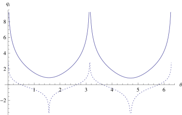
Figure 1: The solutions $q_{i}$ for toroidal surface with $a=3,b=1$. Above (solid) curve shows $q_{x}=q_{y}$ and below (dotted) curve shows $q_{z}$

Case 3: motion on quadric surfaces and a general 2D surface Let us study the following standard form with $a$, $b$, and $c$ taking fixed positives, mitweb

$$f(x,y,z)=\frac{x^{2}\alpha}{a^{2}}+\frac{y^{2}\beta}{b^{2}}+\frac{z^{2}\gamma}{c^{2}}-\delta\text{, and }f(x,y,z)=0,$$ (27)

where parameters $\alpha,\beta,\gamma$ take values either $-1$, $0$ or $1$ and $\delta$ takes values either $0$ or $1$, depending on the classification of quadrics containing six basic quadric surfaces such as ellipsoids, hyperboloids of one and two sheets, elliptic cones, elliptic cylinders and hyperbolic cylinders. mitweb Some quadric surfaces such as elliptic paraboloid and hyperbolic paraboloid, etc. does not belong to the six basic quadric surfaces, but can be treated in similar way. In this Letter, we are only interested in cases with nonvanishing Gaussian curvature $K$, i.e.,

$$K=\alpha\beta\gamma\delta\left\{abc\left(\frac{\left(\alpha x\right)^{2}}{a^{4}}+\frac{\left(\beta y\right)^{2}}{b^{4}}+\frac{\left(\gamma z\right)^{2}}{c^{4}}\right)\right\}^{-2}\neq 0,\text{ }\alpha\beta\gamma\delta\neq 0.$$ (28)

GCFL (2) now gives a very compact equation,

$$\mathbf{\dot{p}=}-\mathbf{n}\frac{\sqrt{abc}}{\mu}\left(\frac{K}{\alpha\beta\gamma\delta}\right)^{1/4}\left(\alpha\frac{p_{x}^{2}}{a^{2}}+\beta\frac{p_{y}^{2}}{b^{2}}+\gamma\frac{p_{z}^{2}}{c^{2}}\right).$$ (29)

Here we like to mention another interesting appearance of the $K^{1/4}$ in Electrostatics. The charge density of the isolated conductors whose surfaces are quadric is also proportional to it. kmliu ; chargedensity After many years’ exploration, we know that the ”local” charge density does not depend on the local geometric properties only. chargedensity The same conclusion applies for the GCFL with a general $2D$ surface $f(\mathbf{x})=0$. It is straightforward to prove following equation,

$$\mathbf{\dot{p}=}-\mathbf{n}\sum_{i=1}^{3}\left\{\left(\frac{f_{ii}^{\prime\prime}}{f_{i}^{\prime}}+f_{i}^{\prime}\frac{f_{jk}^{\prime\prime}}{f_{j}^{\prime}f_{k}^{\prime}}\right)f_{i}^{\prime}-\left(\frac{f_{ik}^{\prime\prime}}{f_{k}^{\prime}}+\frac{f_{ij}^{\prime\prime}}{f_{j}^{\prime}}\right)f_{i}^{\prime}\right\}p_{i}^{2}$$ (30)

where the subscripts ($j,k$) in the $i$-th curly bracket $\left\{{}\right\}$ before $p_{i}^{2}$ differ from each other $i\neq j\neq k$. Evidently, there is no simple relationship between the force $\mathbf{\dot{p}}$ at a point and its curvatures of the point, with known expressions for mean and Gaussian curvature. implicit

During performing quantization, we find that each term of the RHS (30) can be divided into two noncommuting factors, $Q_{i}(\mathbf{x})\equiv\mathbf{n}\left\{\left(\frac{f_{ii}^{\prime\prime}}{f_{i}^{\prime}}+f_{i}^{\prime}\frac{f_{jk}^{\prime\prime}}{f_{j}^{\prime}f_{k}^{\prime}}\right)f_{i}^{\prime}-\left(\frac{f_{ik}^{\prime\prime}}{f_{k}^{\prime}}+\frac{f_{ij}^{\prime\prime}}{f_{j}^{\prime}}\right)f_{i}^{\prime}\right\}$ and $p_{i}^{2}$. We find that the ”dummy” factors $e^{\pm q_{i}(x)}$ allowing for both the geometric momentum and potential satisfy following three equations,

$$\left[p_{i}\mathbf{,}H\right]=-i\hbar\sum_{i=1}^{3}\left(e^{-q_{i}(x)}Q_{i}(\mathbf{x})p_{i}^{2}e^{q_{i}(x)}+e^{-q_{i}(x)}p_{i}^{2}Q_{i}(\mathbf{x})e^{-q_{i}(x)}\right),(i=1,2,3).$$ (31)

The explicit forms of these differential equations are available but extremely lengthy. The closed form solutions are mathematically forbidden.

Conclusions and discussions For the motion on the $2D$ surface, the GCFL $\mathbf{\dot{p}=}\left[\mathbf{p,}H_{c}\right]$ can never be automatically satisfied in quantum mechanics as $\left[\mathbf{p,}H\right]=i\hbar\left[\mathbf{p,}H_{c}\right]$. This difficulty originates from at least two respects: 1) the confining technique implies that in quantum mechanics, $H=\mathbf{p}^{2}/2\mu$ does no longer hold true, and has additional curvature-induced quantum potential. 2) The interplay between the geometric quantities and the kinematic ones $p_{i}$ and $L_{i}$ has different forms in classical mechanics, which are not equivalent to each other in quantum mechanics. In order to resolve the difficulty, we slightly enlarge the canonical quantization scheme which contains not only the fundamental ones $\left[\mathbf{x,x}\right]$, $\left[\mathbf{x,p}\right]$ and $\left[\mathbf{p,p}\right]$, but also $\left[\mathbf{x,}H\right]$ and $\left[\mathbf{p,}H\right]$, which constitute that minimum set to simultaneously determine the operators $\mathbf{x,p}$ and $\mathbf{H}$. Then we demonstrate that within the Dirac canonical quantization scheme the geometric momentum and potential are simultaneously admissible with use of the constrain condition $f(\mathbf{x})=0$. Thus, the difficulty is explicitly settled down for motion constrained on the $2D$ surfaces. In addition, we find that there is no simple relationship between the force on a point of the surface and its curvatures, in sharp contrast to the usual centripetal force law for motion constrained on the curve. Our work implies that within the Dirac canonical quantization scheme, quantum mechanics for constrained motion admits more complicate forms of curvature-induced energy.

References

• (1) H. Jensen and H. Koppe, Ann. Phys. 63, 586(1971).
• (2) R. C. T. da Costa, Phys. Rev. A 23, 1982(1981).
• (3) G. Ferrari and G. Cuoghi, Phys. Rev. Lett. 100, 230403 (2008).
• (4) Q. H. Liu, L. H. Tang, D. M. Xun, Phys. Rev. A 84, 042101(2011).
• (5) Q. H. Liu, J. Phys. Soc. Jpn. 82, 104002(2013).
• (6) A. Szameit, et. al, Phys. Rev. Lett. 104, 150403(2010).
• (7) J. Onoe, T. Ito, H. Shima, H. Yoshioka and S. Kimura, Europhys. Lett. 98, 27001(2012).
• (8) P. A. M. Dirac, The principles of quantum mechanics, 4th ed Oxford Univ, Oxford, (1967), pg. 87, 112-114
• (9) P. A. M. Dirac, Lectures on quantum mechanics, Yeshiva Univ, NY, (1964), pg. 40-66
• (10) T. Homma, T. Inamoto, and T. Miyazaki, Phys. Rev. D 42, 2049(1990).
• (11) M. Ikegami, Y. Nagaoka, S. Takagi, and T. Tanzawa, Prog. Theor. Phys. 88, 229(1992).
• (12) S. Matsutani, J. Phys. A: Math. Gen. 26, 5133(1993).
• (13) H. Kleinert, and S. V. Shabanov, Phys. Lett. A 232, 327(1997).
• (14) D. M. Xun, Q. H. Liu, X. M. Zhu, Ann. Phys. (NY) 338, 123–133(2013).
• (15) D. M. Xun, Q. H. Liu, Ann. Phys. (NY), 341, 132–141(2014).
• (16) S. Weinberg, Lectures on Quantum Mechanics, 2nd ed., (Cambridge University Press, Cambridge U.K. 2015), pg. 335-340.
• (17) P. A. M. Dirac, Proc. Roy. Soc. (London), A. 109 642-653(1925).
• (18) Q. H. Liu, J. Math. Phys. 54, 122113(2013).
• (19) Z. S. Zhang, S. F. Xiao, D. M. Xun, and Q. H. Liu, Commun. Theor. Phys. 63, 19-24(2015)
• (20) In present study, on one relation $\left[\mathbf{p,}H\right]=i\hbar O\left(\left[\mathbf{p,}H_{c}\right]\right)$ is explicitly utilized.
• (21) The first appearance of geometric momentum can be traced back to 1968, exploring the full dynamical group for particles on $2D$ spherical surface: G. Gyorgyi, S. Kovesi-Domokos, IL Nuovo Cimento B, 58, 191(1968). The geometric momentum for a $nD$ ($n=1,2,3...$) spherical surfaces: Y. Ohnuki and S. Kitakado, J. Math. Phys. 34, 2827 (1993). See also, homma ; ikegami
• (22) If only the commutation relations between $[\mathbf{p,}H]$ are required, it is not necessary to utilize the Dirac’s theory of constrained systems.
• (23) http://web.mit.edu/hyperbook/Patrikalakis-Maekawa-Cho/node33.html, http://tutorial.math.lamar.edu/Classes/CalcIII/QuadricSurfaces.aspx.
• (24) H. Kleinert, Path Integrals in Quantum Mechanics, Statistics, Polymer Physics, and Financial Markets, 5th ed., (World Scientific, Singapore, 2009). In this monograph, Kleinert introduced the ”dummy factors” when quantizing a classical Hamiltonian.
• (25) K. M. Liu, Am. J. Phys. 55 849–852(1987).
• (26) D. J. Cross, J. Math. Phys., 55, 123504 (2014).
• (27) R. Goldman, Computer Aided Geometric Design 22, 632–658(2005).