Fingerprints of Majorana fermions in spin-resolved subgap spectroscopy

Abstract

When a strongly correlated quantum dot is tunnel-coupled to a superconductor, it leads to the formation of Shiba bound states inside the superconducting gap. They have been measured experimentally in a superconductor-quantum dot-normal lead setup. Side coupling the quantum dot to a topological superconducting wire that supports Majorana bound states at its ends, drastically affects the structure of the Shiba states and induces supplementary in-gap states. The anomalous coupling between the Majorana bound states and the quantum dot gives rise to a characteristic imbalance in the spin resolved spectral functions for the dot operators. These are clear fingerprints for the existence of Majorana fermions and they can be detected experimentally in transport measurements. In terms of methods employed, we have used analytical approaches combined with the numerical renormalization group approach.

I Introduction

Majorana bound states (MBSs) Alicea et al. (2011); Alicea (2012) are zero energy states that appear at the ends of a topological superconductor with broken spin degeneracy. During the last few years, there have been many proposals on how to probe the MBSs. Signatures of MBSs have been found in ferromagnetic atomic chains assembled on the surface of superconducting lead (Pb) Nadj-Perge et al. (2014), in one dimensional semiconducting wires Das et al. (2012), in hybrid semiconductor-superconductor structures Rokhinson et al. (2012); Mourik et al. (2012), or at the vortex core inside a topological insulator superconductor heterostructure Xu et al. (2015). One of their distinctive features is the zero bias anomaly in tunneling experiments Law et al. (2009); Sau et al. (2010). On the other hand, this is also a hallmark for other phenomena, such as the Kondo effect in quantum dots (QD) Goldhaber-Gordon et al. (1998), the ’0.7 anomaly’ in a point contact Rejec and Meir (2006), and the formation of the Shiba bound states in a superconductor-QD-normal metal (S-QD-N) setup De Franceschi et al. (2010); Deacon et al. (2010). It is present even in systems where the Kondo effect and superconductivity compete Buitelaar et al. (2002). Therefore, finding ways for the clear confirmation of MBSs is a difficult task.

When the same experimental response can be triggered by different phenomena, one promising route to differentiate between them is to study systems that can capture them both. Such an interplay between the in-gap Shiba states and the MBSs has been successfully investigated in Ref. Nadj-Perge et al. (2014).

In the present work, following this route, we propose and study theoretically a tunable setup in which the Shiba bound states can hybridize with the MBSs. The device is presented in Fig. 1 and consists of a QD side coupled to a topological superconducting wire (TSW) that supports MBSs near its ends. The QD is embeded between a BCS superconductor and a normal lead, forming a S-QD-N setup Deacon et al. (2010). It is assumed that the QD is weakly coupled to the normal lead (no Kondo correlations are formed on the normal side as the corresponding Kondo temperature $T_{K}^{(N)}$ is exponentially suppressed), and strongly coupled to the superconductor ($\Gamma_{S}\gg\Gamma_{N}$). In the absence of the TSW, this system has been thoroughly investigated by now, both experimentally Deacon et al. (2010); Lee et al. (2012, 2013); Kumar et al. (2014); Zitko et al. (2015) and theoretically Shiba (1968); Rozhkov and Arovas (1999); Meng et al. (2009); Mart n-Rodero and Yeyati (2012); Zonda et al. (2015). It presents two distinctive phases, i.e., a doublet and a singlet Matsuura (1977) separated by a quantum phase transition (QPT). Furthermore, the evolution of the subgap Shiba states as function of the gate voltage was successfully mapped by conductance measurements, and the agreement with the theoretical predictions is outstanding Deacon et al. (2010).

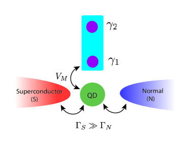
Figure 1: (Color online) Sketch with the setup. An interacting quantum dot (QD) is embedded between a superconductor and a normal lead and is side-coupled to a a topological superconducting wire that supports two Majorana modes $\gamma_{1}$ and $\gamma_{2}$ at the ends. The QD is strongly coupled to the superconductor, and weakly coupled to the normal lead, i.e., $\Gamma_{S}\gg\Gamma_{N}$.

We have found that if a TSW is attached to the QD, as in Fig. 1, the in-gap spectrum gets substantially modified by the presence of the MBSs. Moreover, by investigating the spectral functions for the QD operators, we have found a strong characteristic imbalance in the spin resolved spectrum in the vicinity of the QPT, which in principle can be measured experimentally by performing spin polarized tunneling measurements. Our findings indicate that such a device may provide clear fingerprints for the presence of the MBSs. In terms of the methods we used, our analytical estimates have been supplemented by state of the art numerical renormalization group (NRG) calculations Wilson (1975); Krishna-murthy et al. (1980).

II The Model

We consider a QD that is coupled to a TSW. The QD itself is described by a single spinful interacting level with energy $\varepsilon$ and Coulomb repulsion $U$:

$$H_{\rm D}=\varepsilon\sum_{\sigma}d_{\sigma}^{\dagger}d_{\sigma}+U{\hat{n}}_{\uparrow}{\hat{n}}_{\downarrow}\,.$$ (1)

Here $d_{\sigma}^{\dagger}$ is the creation operator for an electron with spin $\sigma$ in the dot and $\hat{n}_{\sigma}$ is the occupation operator in the spin-$\sigma$ sector. Although the TSW is a complicated mesoscopic object, it has been shown in Ref. Alicea et al. (2011); Ruiz-Tijerina et al. (2015) that it is possible to construct an effective model that captures the essential physics of the QD-TSW by representing the wire in terms of its Majorana end states

$$H_{M} = i\,\varepsilon_{M}\gamma_{1}\gamma_{2}=\varepsilon_{M}(1+f^{\dagger}f)\,,$$ (2)

where $\gamma_{1}=1/\sqrt{2}(f+f^{\dagger})$, $\gamma_{2}=i/\sqrt{2}(f-f^{\dagger})$ are the operators for the MBSs at the ends of the wire, and $f$ and $f^{\dagger}$ are some regular fermionic operators associated with the MBSs. The former satisfy the anticommutation relations $\{\gamma_{1},\gamma_{2}\}=0$, while $\gamma_{1}^{2}=\gamma_{2}^{2}=1$. In our configuration we consider the mode $\gamma_{2}$ to reside at the far end of the wire such that only $\gamma_{1}$ hybridizes with the states in the dot (see Fig. 1) and may even leak into the dot Vernek et al. (2014). When the TSW is in the topological phase, we assume that due the orientation of the Zeeman field in the TSW Alicea et al. (2011); Ruiz-Tijerina et al. (2015), only the spin-down channel of the dot is coupled to $\gamma_{1}$

$$H_{D-M} = V_{M}(d^{\dagger}_{\downarrow}\gamma_{1}+\gamma_{1}d_{\downarrow})\,,$$ (3)

with $V_{M}$ the tunneling amplitude between the QD and MBS. The effective model that describes the QD-TSW is then given by

$$H_{\rm eff}=H_{\rm D}+H_{\rm M}+H_{\rm D-M}.$$ (4)

To capture the interplay between the MBSs and the Shiba states, the QD is embedded between a BCS superconductor on one side and a normal lead on the other side. In such a S-QD-N setup, the Shiba states Shiba (1968) are well resolved in the local spectral functions as long as $\Gamma_{S}\gg\Gamma_{N}$, with $\Gamma_{N(S)}/\hbar$ the superconducting (normal) tunneling rates. If $\Gamma_{N}\ll\Delta$, the Kondo temperature $T_{K}^{N}$ (due to the coupling to the normal lead) is vanishingly small, and the S-QD-N setup is qualitatively analogous with a S-QD system, with the normal lead acting simply as a probe (such as the tip of a STM) Deacon et al. (2010). The superconducting lead is described by the BCS Hamiltonian

$$H_{\rm S} = \sum_{{\bf k},\sigma}\xi_{{\bf k}\sigma}c^{\dagger}_{{\bf k}\sigma}c_{{\bf k}\sigma}-(\Delta\,c^{\dagger}_{{\bf k}\uparrow}c^{\dagger}_{-{\bf k}\downarrow}+\mathrm{H.c.})\,.$$ (5)

The first term describes free fermions with dispersion $\xi_{{\bf k}\sigma}$ and the second one the superconducting correlations with the superconducting gap $\Delta$. The conduction band ranges from -D to D and the density of states is considered to be constant, $\rho_{0}=1/2D$. Within our numerical calculations, $D$ is considered to be the energy unit.

The coupling of the dot to the superconducting lead is described by the Hamiltonian

$$H_{\rm tun} = \sum_{\mathbf{k},\sigma}V(d^{\dagger}_{\sigma}c_{\mathbf{k}\sigma}+c^{\dagger}_{\mathbf{k}\sigma}d_{\sigma})\,,$$ (6)

where the tunneling rate between the QD and the normal superconductor $\Gamma=\Gamma_{S}=\pi\rho_{0}V^{2}$. Eqs. (4), (5) and (6) define our model Hamiltonian

$$H=H_{\rm eff}+H_{\rm S}+H_{\rm tun}$$ (7)

In what follows, we neglect the direct coupling between the Majorana lead with the normal superconductor, as well as the coupling between the QD and the p-wave continuum in the TSW.

III Superconducting atomic limit, $\Delta\to\infty$

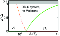
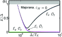
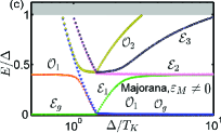
Figure 2: (Color online) Analytical and NRG results for the energy spectrum in different configurations. (a) Bound states in the atomic limit for the S-QD setup, without an attached TSW. The energies are those corresponding to Eq. (10). (b) The energy spectrum when the TSW is coupled to the QD and the Majorana level has an energy $\varepsilon_{M}=0$. As the ground state has no particular symmetry, the QPT is absent. (c) The evolution of the energy spectrum when $\varepsilon_{M}=0.4\,\Delta$. The level ${\cal O}_{1}$ becomes degenerate with ${\cal O}_{g}$ in the $\Delta/T_{K}\to\infty$ limit. (d) Similar to (c) but computed exactly with the NRG. Notice that we represent the evolution of the bound states on a wider $\Delta/T_{K}$ range. In all the plots, the parameters are: $V_{M}/\Delta=0.1$ and $U/\Delta=-2\varepsilon/\Delta=3$. The shaded region above $\Delta$ represents the continuum.

The model Hamiltonian introduced in Eq. (7) can not be solved exactly in general. In the absence of the TSW, the Hamiltonian reduces to $H=H_{\rm D}+H_{\rm S}+H_{\rm tun}$, and the problem can be solved exactly by using the numerical renormalization group approach Wilson (1975); Krishna-murthy et al. (1980). Analytically, the limiting case $\Delta\to\infty$, i.e., the superconducting atomic limit, has been addressed in several studies  Meng et al. (2009); Bauer et al. (2007); Oguri et al. (2004); Tanaka et al. (2007). By integrating the superconducting lead we can construct an effective Hamiltonian that captures the essential physics. When the TSW is present, the Hamiltonian reads

$$H_{\rm el}^{(\Delta\to\infty)}=\sum_{\sigma}\xi_{d}\,d^{\dagger}_{\sigma}d_{\sigma}-\Gamma_{\varphi}\left(d^{\dagger}_{\uparrow}d^{\dagger}_{\downarrow}+\mathrm{H.c.}\right)+\\ +{U\over 2}\left({\hat{n}}-1\right)^{2}+H_{M}+H_{D-M}.$$ (8)

Here, $\xi_{d}=\varepsilon+U/2$ and $\Gamma_{\varphi}=2\,\Gamma/\pi\arctan\left(D/\Delta\right)$. The superconducting correlations are embedded in the second term in Eq. (8), which corresponds to a local pairing term induced by superconductivity in the dot. In what follows we shall restrict ourselves to the symmetric case $\varepsilon=-U/2$, but our main results also hold in the general case. Although more elaborate analytical models can be constructed Zonda et al. (2015), this simple model captures qualitatively all the important features, as demonstrated by a comparison with NRG calculations. The Hamiltonian (8) can be diagonalized exactly and has in general eight non-degenerate eigenstates.

To get a clear picture, let us first discuss what happens in the absence of the TSW. In this case, the system has a global $SU(2)\times Z_{2}$ symmetry corresponding to the conservation of the total spin in the dot (the Majorana modes have no spin index) and to the parity of the state . This allows us to organize the states in spin multiplets. There are only four eigenstates that can be grouped into a pair of singlets $|{\cal S}_{\pm}\rangle$ and a doublet $|{\cal D}_{\sigma}\rangle$:

$$|{\cal S}_{\pm}\rangle =1/\sqrt{2}(\pm d^{\dagger}_{\uparrow}\,d^{\dagger}_{\downarrow}+1)|0\rangle\,,$$ (9a)

$$|{\cal D}_{\sigma}\rangle =d^{\dagger}_{\sigma}|0\rangle\,.$$ (9b)

The corresponding eigenenergies are

$$E_{\pm} = U/2\pm\Gamma_{\varphi}\,,\;\;\;E_{\sigma}=0\,.$$ (10)

One notices that $E_{+}$ is always larger than $E_{-}$, and that the crossing point corresponding to $E_{-}=E_{\sigma}$ signals a quantum phase transition (QPT), as the parity of the ground state changes. Although the QPT is captured in this simple local model, the true nature of the QPT is due to the competition between the Kondo screening and the superconducting correlations and happens at $\Delta\sim T_{K}$, with $T_{K}$ the Kondo scale . Strictly speaking, the atomic limit is exact when $\Delta\to\infty$, but comparisons with the exact NRG results indicate that the superconducting atomic limit is a good approximation as long as $\Delta$ is the largest energy scale in the problem. In Fig. 2(a) we represent the evolution of the Shiba states in the absence of the TSW as function of $\Delta/T_{K}$. When $\Delta\ll T_{K}$ the ground state is the singlet $|\cal S_{-}\rangle$, while in the opposite limit, $\Delta\gg T_{K}$, the ground state changes to the doublet $|\cal D_{\sigma}\rangle$. Such subgap resonances have been already measured in transport experiments in Refs. Deacon et al. (2010); De Franceschi et al. (2010) with good agreement with the theoretical predictions.

When $V_{M}\neq 0$ but $\varepsilon_{M}=0$, the global $SU(2)$ spin symmetry is completely lost and the states can be organized by parity only (see Appendix A for explicit expressions). In what follows, we shall label ${\cal E}_{i}({\cal O}_{i})$, with $i=g,1,2,\dots$ the states in the even (odd) sectors. If $U$ is sufficiently large compared to $\Delta$, the highest two energy levels will be in the continuum and only six states lie inside the gap (see Fig. 2(b)). They come in pairs such that each even state is degenerate in energy with an odd state. Since the ground state has no defined parity, the QPT is completely washed away. In this limit, the spectral function of the $d^{\dagger}_{\uparrow}$-operator in the QD shows a resonance pinned at $\omega=0$ which corresponds to the ${\cal E}_{g}\leftrightarrow{\cal O}_{g}$ transition (see Fig 3(b)). We expect this transition to be visible in the differential conductance across the dot in the whole $\Delta/T_{K}$ domain Deacon et al. (2010). Keeping $\Gamma_{N}$ small enough, we rule out any possible Kondo correlations that would give a similar signal.

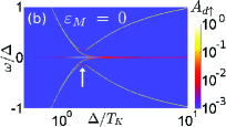
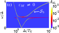
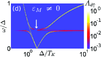
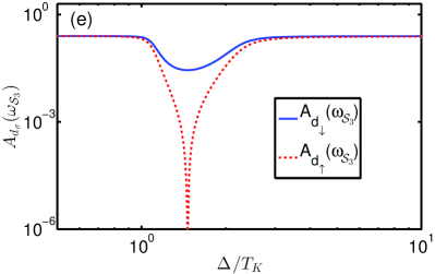
Figure 3: (Color online) Panels (a-b): Evolution of the spectral functions $A_{d_{\downarrow}}(\omega)$ and $A_{d_{\uparrow}}(\omega)$ in the subgap region $|\omega|<\Delta$ for $\varepsilon_{M}=0$. (c-d) The same as in (a-b) but for finite $\varepsilon_{M}=0.4\;\Delta$, represented only in the positive frequency domain $0<\omega<\Delta$. The spectral functions present electron-hole symmetry, and the spectra for the positive and negative frequencies are symmetrical. (e) Evolution of the peak weights for $A_{d_{\sigma}}(\omega_{{\cal S}_{3}})$ as we follow the ${\cal S}_{3}$ resonance indicated in panel (c). At the QPT, the spin-$\uparrow$ weight vanishes. The white arrows in panels (b) and (d) indicate where the spin imbalance takes place. In all the panels, the results are analytical estimates in the atomic limit (see Appendix A for details). Similar results (not displayed here) are obtained with the NRG approach.

In general, we can assume that the Majorana fermion may have a finite energy $\varepsilon_{M}$, which is related to the physical length $L$ and the coherence length $\zeta$ of the TSW, and scales as $\varepsilon_{M}\propto E\exp(-L/\zeta)$ Alicea (2012); Dumitrescu et al. (2015), where $E$ is given by the product of the induced gap and the momentum at the Fermi level Brouwer et al. (2011). In current experiments, $\varepsilon_{M}$ is likely in the range 100-200 mK Sarma et al. (2015), however it can in principle be adjusted by changing the parameters that affect the coherence length and control the transition to the topological phase, such as the Zeeman splitting or the chemical potential. In this case, the states ${\cal E}_{i}$ and ${\cal O}_{i}$ are no longer degenerate in energy and the QPT is restored. When $\Delta\sim T_{K}$, the ground state changes from an even to an odd state. The energy spectra can again be found analytically. Their evolution is presented in Fig. 2(c). We have found that the MBS presents unique signatures when compared with other possible configurations (not presented here). Thus, when the MBSs are for example replaced by a resonant level with an on-site $U=\infty$, the system has a restored $U(1)$ symmetry corresponding to the conservation of $S_{z}$, and the energy spectrum is affected significantly. For the sake of completeness, we present in Fig. 2(d) the energy spectrum using the same set of parameters as those in panel (c), but computed with the NRG approach. The agreement between the results guarantees the correctness of the superconducting atomic limit.

IV Spectral Functions

The energy spectrum discussed so far can be captured in subgap spectroscopy when the normal lead is weakly coupled to the dot, i.e., $\Gamma_{N}\ll\Gamma_{S}$. Recently, signatures of the MBSs formed inside a vortex core in a $\rm Bi_{2}Te_{3}/NbSe_{2}$ heterostructure have been detected by using spin-polarized scanning tunneling spectroscopy (SP-STS) Sun et al. (2016). They have been revealed by measuring the differences in the differential conductance with the tip magnetization aligned along/against the local magnetic field. In our setup, the coupling between the TSW and the QD is spin-selective, as only the spin-$\downarrow$ channel is coupled to the MBSs. Then, we expect a similar imbalance in the spin resolved spectral functions. This imbalance can be observed by performing spin-polarized transport measurements by replacing the normal lead with a ferromagnetic one in the setup presented in Fig. 1.

In this section we discuss the results for the spin-polarized spectral functions $A_{d_{\sigma}}(\omega)$ of the operators $d^{\dagger}_{\sigma}$ describing the excitations in the dot. They are defined as

$$A_{d_{\sigma}}(\omega)=-{1\over\pi}\rm{Im}\,G_{d_{\sigma}}(\omega)\,,$$ (11)

with $G_{d_{\sigma}}(\omega)$ being the Fourier transform of the retarded electronic Green’s function: $G_{d_{\sigma}}(t)=-i\theta(t)\langle\{d_{\sigma}(t),d^{\dagger}_{\sigma}\}\rangle$. We present results for zero temperature, in which case $A_{d_{\sigma}}(\omega)$ captures transitions between the ground state and the excited Shiba states having different parities. Moreover, we are interested in distinctive characteristics due to the coupling to the MBS, so that we discuss only the subgap spectrum $\omega<\Delta$. In Fig. 3(a,b) and Fig. 3(c,d) we represent the spin resolved spectral functions $A_{d_{\sigma}}(\omega)$ for $\varepsilon_{M}=0$ and for finite $\varepsilon_{M}$ respectively. All the results presented in Fig. 3 were obtained analytically within the atomic limit. For the sake of completeness, we have also performed NRG calculations (not displayed here) that confirm the main features. The expressions for the energy eigenstates and the matrix elements of the $d_{\sigma}$ operator are given in Appendix A. The Shiba states are mixed with the MBSs, and together they form the localized states inside the gap. Therefore, they contribute with similar weights to the transitions captured by the spectral functions. Moreover, the excited states with the same symmetry lead to the formation of avoided crossings on either side of the QPT. The spectral functions present two distinctive features: (i) For $\varepsilon_{M}=0$, the spectral function $A_{d_{\uparrow}}(\omega)$ always shows a resonance at $\omega=0$, which is due to the ${\cal E}_{g}\leftrightarrow{\cal O}_{g}$ transition, while $A_{d_{\downarrow}}(\omega)$ does so only asymptotically in the large $\Delta/T_{K}$ limit (in the non-symmetric case, $\varepsilon\neq-U/2$, both spectral functions have a resonance at $\omega=0$); (ii) For both finite and vanishing $\varepsilon_{M}$, there is a small window close to the QPT, where the transition between the ground state and the third excited Shiba state, ${\cal E}_{g}\leftrightarrow{\cal O}_{3}$ or ${\cal O}_{g}\leftrightarrow{\cal E}_{3}$, becomes strongly spin-polarized. This region is indicated by the arrow in Fig.  3(b, d). Following this resonance, the weight of the spectral function for the spin-$\uparrow$ channel vanishes close to the QPT. This is shown in Fig. 3(e), where we represent the weighs for $A_{d_{\sigma}}(\omega_{{\cal S}_{3}})$ at the resonance frequency as we follow the ${\cal O}_{3}$ and ${\cal S}_{3}$ resonance.

We want to highlight the fact that this behavior is a clear signature of the Majorana fermions, and is due to the existence of the anomalous hopping term in Eq. (3) that simultaneously creates (annihilates) two quasiparticles, one on the dot and one on the TSW. Moreover, no such behavior is expected when the QD is side-coupled to a resonant level or to a second QD, for example.

V Concluding Remarks

A quantum dot coupled to a normal superconductor shows characteristic resonant features in the subgap spectrum. These are known as Shiba bound states and have been measured in tunneling spectroscopy experiments Deacon et al. (2010). Such a system has two distinct phases separated by a quantum phase transition.

Majorana fermions are particles that are their own antiparticles, and have been predicted in condensed matter systems Alicea (2012), and in particular as localized states at the ends of a topological wire. Their signature is associated with the existence of a zero energy mode, and has been confirmed experimentally in various experiments Nadj-Perge et al. (2014); Xu et al. (2015); Mourik et al. (2012).

In the present work we propose a setup in which clear fingerprints of the Majorana modes can be detected by using spin-resolved tunneling spectroscopy measurement. We have investigated the changes in the subgap spectrum when the quantum dot is side-coupled to such a topological wire. We have found distinctive hallmarks that can be associated only with Majorana bound states. In particular, we have found that when the two Majorana modes at the ends of the topological wire are completely decoupled, the quantum phase transition is washed away, but a finite coupling between them restores the phase transition. Moreover, in the vicinity of the quantum phase transition, the spin resolved spectrum for the dot operators becomes strongly spin-polarized.

Appendix A Analytical results in the atomic limit

In this appendix we present analytical details for the calculation of the energy spectrum and for the transition amplitudes of the $d_{\sigma}$-operators between these states. These quantities are needed for the calculation of the spectral functions, which are discussed in Sec. IV. In the atomic limit, the Hamiltonian (8) can be diagonalized exactly. Altogether, there are eight states, but only six of them reside inside the gap, the other two merging with the continuum. We shall consider the electron-hole symmetrical case, i.e, $\varepsilon=-U/2$, for which simple analytical expressions can be found. We shall focus here on the region $\Delta/T_{K}\gg 1$, where the ground state resides in the odd sector. The corresponding six eigenenergies are

$$E^{{\cal O}}_{i=g,1,2} = \frac{1}{4}\left(U+2\eta_{i1}\Gamma_{\varphi}+2\varepsilon_{M}+\right.$$

$$\left.+\eta_{i2}\sqrt{8V_{M}^{2}+(U+2\eta_{i1}\Gamma_{\varphi}+2\varepsilon_{M})^{2}}\right)\,,$$

$$E^{{\cal E}}_{i=1,2,3} = \frac{1}{4}\left(U+2\eta_{i2}\Gamma_{\varphi}+2\varepsilon_{M}+\right.$$

$$\left.+\eta_{i3}\sqrt{8V_{M}^{2}+(U+2\eta_{i2}\Gamma_{\varphi}-2\varepsilon_{M})^{2}}\right)\,,$$

where the upper superscripts $\{\cal E,\cal O\}$ label the even and respectively odd states, and we introduced the notation $\eta_{ij}=-1+2\delta_{ij}$, with $\delta_{ij}$ the Kroenecker symbol. Depending on the ratio $\Delta/T_{K}$, the ground state changes from an even to an odd state across the QPT point. The energies have to be rescaled so that the ground state has zero energy.

At the same time, we can obtain the eigenstates exactly. Within the basis $\{$ $|0\rangle,|\uparrow\rangle,|\downarrow\rangle,|\uparrow\downarrow\rangle\}\otimes\{|0_{M}\rangle,|1_{M}\rangle$ $\}$, formed out of the dot and Majorana states, the eigenvectors are given by

$$|{\cal E}_{i=1,2,3}\rangle=\frac{1}{\sqrt{2(u_{{\cal E}_{i}}^{2}+1)}} \left(u_{{\cal E}_{i}}\left(|0\rangle-\eta_{i2}|\uparrow\downarrow\rangle\right)|0_{M}\rangle+\right.$$

$$\left.+\left(-\eta_{i2}|\uparrow\rangle+|\downarrow\rangle\right)|1_{M}\rangle\right)\,,$$

$$|{\cal O}_{i=g,1,2}\rangle=\frac{1}{\sqrt{2(u_{{\cal O}_{i}}^{2}+1)}} \left(u_{{\cal O}_{i}}\left(|\uparrow\rangle-\eta_{i1}|\downarrow\rangle\right)|0_{M}\rangle+\right.$$

$$\left.+\left(-\eta_{i1}|0\rangle+|\uparrow\downarrow\rangle\right)|1_{M}\rangle\right)\,,$$

where we used the short hand notations

$$u_{{\cal E}_{i=1,2,3}}= \frac{1}{2\sqrt{2}V_{M}}\left(U+2\eta_{i2}\Gamma_{\varphi}-2\varepsilon_{M}+\right.$$

$$\left.+\eta_{i3}\sqrt{8V_{M}^{2}+(U+2\eta_{i2}\Gamma_{\varphi}-2\varepsilon_{M})^{2}}\right)\,,$$

$$u_{{\cal O}_{i=g,1,2}}= 2\sqrt{2}V_{M}/\left(U+2\eta_{i1}\Gamma_{\varphi}+2\varepsilon_{M}+\right.$$

$$\left.+\eta_{i2}\sqrt{8V_{M}^{2}+(U+2\eta_{i1}\Gamma_{\varphi}+2\varepsilon_{M})^{2}}\right)\,.$$

This allows us to compute the matrix elements for the operators in the dot. Since $d_{\sigma}$ is a charge Q=1 operator, only transitions between states with different symmetry are allowed. Furthermore, since the Majorana mode couples only to the spin-$\downarrow$ channel, the matrix elements for $d_{\uparrow}$ and $d_{\downarrow}$ are different. For example: $\langle{\cal{O}}_{g}|d_{\uparrow}|{\cal{E}}_{3}\rangle=(1+u_{{\cal{E}}_{3}}u_{{\cal{O}}_{g}})/2\sqrt{(u_{{\cal{E}}_{3}}^{2}+1)(u_{{\cal{O}}_{g}}^{2}+1)}$ and $\langle{\cal{O}}_{g}|d_{\downarrow}|{\cal{E}}_{3}\rangle=(1-u_{{\cal{E}}_{3}}u_{{\cal{O}}_{g}})/2\sqrt{(u_{{\cal{E}}_{3}}^{2}+1)(u_{{\cal{O}}_{g}}^{2}+1)}$. Then, the spectral functions are simply given by

$$A_{d_{\sigma}}(\omega)=|\langle{\cal{O}}_{g}|d_{\sigma}|{\cal{E}}_{3}\rangle|^{2}\delta(\omega+E_{g}^{\cal O}-E_{3}^{\cal E}).$$ (12)

Their evolution across the QPT is represented in Fig. 3(e). Notice that the spin-up spectral function becomes zero at the QPT point corresponding to $U=2\Gamma_{\varphi}$.

References

- Alicea et al. (2011) J. Alicea, Y. Oreg, G. Refael, F. von Oppen, and M. P. A. Fisher, Nat Phys 7, 412 (2011).
- Alicea (2012) J. Alicea, Reports on Progress in Physics 75, 076501 (2012).
- Nadj-Perge et al. (2014) S. Nadj-Perge, I. K. Drozdov, J. Li, H. Chen, S. Jeon, J. Seo, A. H. MacDonald, B. A. Bernevig, and A. Yazdani, Science 346, 602 (2014).
- Das et al. (2012) A. Das, Y. Ronen, Y. Most, Y. Oreg, M. Heiblum, and H. Shtrikman, Nat Phys 8, 887 (2012).
- Rokhinson et al. (2012) L. P. Rokhinson, X. Liu, and J. K. Furdyna, Nat Phys 8, 795 (2012).
- Mourik et al. (2012) V. Mourik, K. Zuo, S. M. Frolov, S. R. Plissard, E. P. A. M. Bakkers, and L. P. Kouwenhoven, Science 336, 1003 (2012).
- Xu et al. (2015) J.-P. Xu, M.-X. Wang, Z. L. Liu, J.-F. Ge, X. Yang, C. Liu, Z. A. Xu, D. Guan, C. L. Gao, D. Qian, Y. Liu, Q.-H. Wang, F.-C. Zhang, Q.-K. Xue, and J.-F. Jia, Phys. Rev. Lett. 114, 017001 (2015).
- Law et al. (2009) K. T. Law, P. A. Lee, and T. K. Ng, Phys. Rev. Lett. 103, 237001 (2009).
- Sau et al. (2010) J. D. Sau, S. Tewari, R. M. Lutchyn, T. D. Stanescu, and S. Das Sarma, Phys. Rev. B 82, 214509 (2010).
- Goldhaber-Gordon et al. (1998) D. Goldhaber-Gordon, H. Shtrikman, D. Mahalu, D. Abusch-Magder, U. Meirav, and M. A. Kastner, Nature 391, 156 (1998).
- Rejec and Meir (2006) T. Rejec and Y. Meir, Nature 442, 900 (2006).
- De Franceschi et al. (2010) S. De Franceschi, L. Kouwenhoven, C. Schonenberger, and W. Wernsdorfer, Nat Nano 5, 703 (2010).
- Deacon et al. (2010) R. S. Deacon, Y. Tanaka, A. Oiwa, R. Sakano, K. Yoshida, K. Shibata, K. Hirakawa, and S. Tarucha, Phys. Rev. Lett. 104, 076805 (2010).
- Buitelaar et al. (2002) M. R. Buitelaar, T. Nussbaumer, and C. Schönenberger, Phys. Rev. Lett. 89, 256801 (2002).
- Lee et al. (2012) E. J. H. Lee, X. Jiang, R. Aguado, G. Katsaros, C. M. Lieber, and S. De Franceschi, Phys. Rev. Lett. 109, 186802 (2012).
- Lee et al. (2013) E. J. H. Lee, X. Jiang, M. Houzet, R. Aguado, C. M. Lieber, and S. De Franceschi, Nat Nano 9, 79 (2013).
- Kumar et al. (2014) A. Kumar, M. Gaim, D. Steininger, A. Levy Yeyati, A. Martin-Rodero, A. K. Huttel, and C. Strunk, Phys. Rev. B 89, 075428 (2014).
- Zitko et al. (2015) R. Zitko, J. S. Lim, R. Lopez, and R. Aguado, Phys. Rev. B 91, 045441 (2015).
- Shiba (1968) H. Shiba, Progress of theoretical Physics 40, 435 (1968).
- Rozhkov and Arovas (1999) A. V. Rozhkov and D. P. Arovas, Phys. Rev. Lett. 82, 2788 (1999).
- Meng et al. (2009) T. Meng, S. Florens, and P. Simon, Phys. Rev. B 79, 224521 (2009).
- Mart n-Rodero and Yeyati (2012) A. Mart n-Rodero and A. L. Yeyati, Journal of Physics: Condensed Matter 24, 385303 (2012).
- Zonda et al. (2015) M. Zonda, V. Pokorny, V. Janis, and T. Novotny, Scientific Reports 5, 8821 (2015).
- Matsuura (1977) T. Matsuura, Progress of Theoretical Physics 57, 1823 (1977).
- Wilson (1975) K. G. Wilson, Rev. Mod. Phys. 47, 773 (1975).
- Krishna-murthy et al. (1980) H. R. Krishna-murthy, J. W. Wilkins, and K. G. Wilson, Phys. Rev. B 21, 1003 (1980).
- Ruiz-Tijerina et al. (2015) D. A. Ruiz-Tijerina, E. Vernek, L. G. G. V. Dias da Silva, and J. C. Egues, Phys. Rev. B 91, 115435 (2015).
- Vernek et al. (2014) E. Vernek, P. H. Penteado, A. C. Seridonio, and J. C. Egues, Phys. Rev. B 89, 165314 (2014).
- Bauer et al. (2007) J. Bauer, A. Oguri, and A. C. Hewson, Journal of Physics: Condensed Matter 19, 486211 (2007).
- Oguri et al. (2004) A. Oguri, Y. Tanaka, and A. C. Hewson, Journal of the Physical Society of Japan 73, 2494 (2004).
- Tanaka et al. (2007) Y. Tanaka, A. Oguri, and A. C. Hewson, New Journal of Physics 9, 115 (2007).
- Note (1) At half filling, when , the system presents an extra electron-hole symmetry.
- Note (2) We define by using Haldane’s expression, .
- Note (3) The Majorana mode is coupled to the spin-down channel only, so that the symmetry corresponding to the conservation of is also broken.
- Dumitrescu et al. (2015) E. Dumitrescu, B. Roberts, S. Tewari, J. D. Sau, and S. Das Sarma, Phys. Rev. B 91, 094505 (2015).
- Brouwer et al. (2011) P. W. Brouwer, M. Duckheim, A. Romito, and F. von Oppen, Phys. Rev. Lett. 107, 196804 (2011).
- Sarma et al. (2015) S. D. Sarma, M. Freedman, and C. Nayak, Npj Quantum Information 1, 15001 (2015).
- Sun et al. (2016) H.-H. Sun, K.-W. Zhang, L.-H. Hu, C. Li, G.-Y. Wang, H.-Y. Ma, Z.-A. Xu, C.-L. Gao, D.-D. Guan, Y.-Y. Li, C. Liu, D. Qian, Y. Zhou, L. Fu, S.-C. Li, F.-C. Zhang, and J.-F. Jia, ArXiv e-prints (2016), arXiv:1603.02549 [cond-mat.supr-con] .