Reproducing kernel Hilbert spaces and variable metric algorithms in PDE constrained shape optimisation

Abstract

In this paper we investigate and compare different gradient algorithms designed for the domain expression of the shape derivative. Our main focus is to examine the usefulness of kernel reproducing Hilbert spaces for PDE constrained shape optimisation problems. We show that radial kernels provide convenient formulas for the shape gradient that can be efficiently used in numerical simulations. The shape gradients associated with radial kernels depend on a so called smoothing parameter that allows a smoothness adjustment of the shape during the optimisation process. Besides, this smoothing parameter can be used to modify the movement of the shape. The theoretical findings are verified in a number of numerical experiments.

Keywords: shape optimization; reproducing kernel Hilbert spaces; gradient method; variable metric; radial kernels

AMS classification: 35J15; 46E22; 49Q10; 49K20; 49K40

1 Introduction

Optimal shape design questions naturally arise from problems in the engineering sciences and industrial applications. For instance, it plays an important role in aircraft design, electrical impedance tomography, cantilever designs, inductor coil design and many more. The main objective of shape optimisation is to minimise a certain cost/shape function depending on one or many design variables. A great challenge, relevant for applications, is to find fast and efficient algorithms providing as output (locally) optimal shapes. One may define first and second order methods by means of the so called shape derivative.
A central result of shape optimisation constitutes the structure theorem for shape functions defined on open or closed subsets of the Euclidean space. As a consequence of the structure theorem we can identify, in smooth situations, the shape derivative with a distribution on the boundary only depending on normal perturbations. In many applications this distribution can be written as boundary integral which is referred to as boundary expression. If the shape is not smooth enough one still can conclude that the shape derivative is concentrated on the boundary, but it may not necessarily be a distribution on the boundary anymore. However, for many application problems, a weaker form of the shape derivative is usually available. This form can be referred to as volume/domain expression or distributed shape derivative and it can be written in a convenient tensor form as detailed in [14].
By definition the shape gradient of the shape derivative depends on the choice of the Hilbert space and inner product. It is nothing but the Riesz representation of the shape derivative in this Hilbert space. Using the boundary expression of the shape derivative has the advantage that it allows to resort to boundary spaces. For PDE constrained optimal design problems, many gradient-type algorithms using the boundary expression in conjunction with boundary spaces have been proposed by employing various explicit parametrisations such as Bézier splines, B-splines, NURBS; see e.g. [13, 22, 8, 16, 11, 2]. While the boundary expression gives a relatively easy formula of the shape derivative, it is not the first choice from the numerical point of view as recently pointed out in [12, 14, 4]. By definition the shape gradient depends on the choice of the Hilbert space where the shape derivative is represented. While some choices using $H^{1}$ metrics and finite elements have successfully been used [14, 9], the question arises if there are better Hilbert spaces and metrics that are more controllable. At best, one might want to change the metric during the optimisation process in order to escape stationary points that are no global minima.
Reproducing kernel Hilbert spaces (RKHSs) were introduced in the beginning of the 19th century. They play a crucial role in polynomial approximation and machine learning. We refer to [23] for an introduction to RKHS and their application to scattered data approximation. RKHS can be extended to vector valued reproducing kernel Hilbert spaces (vvRKHS). As shown in [24] they can also efficiently be used to solve diffeomorhpic matching problems. A specific property of vvRKHS is that the point evaluation on them is a continuous linear mapping. Conversely, the continuity of the evaluation mapping in a Hilbert space implies that it is a vvRKHS. The continuity of the evaluation mapping is also necessary to build complete metric groups of diffeomorphisms as demonstrated in [7, Chap. 4]. This shows that there is a close relation between RKHS and shape design problems. Therefore, it seems natural to combine and examine results from RKHS theory with problems from PDE constrained shape optimisation.
In this paper we examine the usefulness of reproducing kernel Hilbert spaces in the context of PDE constrained shape optimisation problems. We combine the generic tensor form of the domain expression of the shape derivative with reproducing kernel Hilbert space methods. We provide ready to use explicit formulas for the shape gradient in these kernel spaces and compare them with previously used ones. Moreover, we study radial kernels that allow us to construct flows that can efficiently detect stationary points. Our theoretical results are verified by several numerical experiments.

Structure of the paper

In Section 2, we review basic results from shape calculus and recall the recently introduced tensor representation of the shape derivative. We recall the definition of the gradient of the shape derivative and define descent directions.

In Section 3, we introduce the theory of reproducing kernel Hilbert spaces and relate them to the shape derivative. Explicit formulas of gradients in general reproducing kernel Hilbert spaces are obtained that can be readily used in numerical algorithms. The general results are specialised to radial kernels and the relation. At the end of the section, different approaches to obtain descent directions are proposed and compared.

In Section 4, a transmission problem together with a tracking-type cost function is studied. We give a detailed description of the discretisation of the PDE and of the shape derivative. In a general tensor setting we compare the discrete domain and boundary expression.

In Section 5, the previously introduced methods are tested in a number of numerical experiments.

2 Preliminaries

In this section, we recall some basics from shape calculus. For an in-depth treatment we refer the reader to the monographs [7, 19, 10]. Numerous examples of PDE constrained shape functions and their shape derivatives can be found in [21].

2.1 Flow of vector fields and shape derivative

Subsequently, let $D\subset\mathbf{R}^{d}$, $d\geq 1$, be an open and bounded set. Given a function $X\in\accentset{\circ}{C}^{0,1}(\mkern 1.5mu\overline{\mkern-1.5muD\mkern-1.5mu}\mkern 1.5mu,\mathbf{R}^{d})$, we denote by $\Phi_{t}$ the flow of $X$ (short $X$-flow) given by $\Phi_{t}(x_{0}):=x(t)$, where $x(\cdot)$ solves

$$x^{\prime}(t)=X(x(t))\qquad\textsf{ in }\qquad(0,\tau],\;x(0)=x_{0}.$$ (2.1)

The space $\accentset{\circ}{C}^{0,1}(\mkern 1.5mu\overline{\mkern-1.5muD\mkern-1.5mu}\mkern 1.5mu,\mathbf{R}^{d})$ comprises all bounded and Lipschitz continuous functions on $\mkern 1.5mu\overline{\mkern-1.5muD\mkern-1.5mu}\mkern 1.5mu$ vanishing on $\partial D$. Note that by the chain rule $\partial\Phi^{-1}(t,\Phi(t,x))=(\partial\Phi(t,x))^{-1}$ which we will often write as

$$(\partial(\Phi^{-1}_{t}))\circ\Phi_{t}=(\partial\Phi_{t})^{-1}=:\partial\Phi^{-1}_{t}.$$ (2.2)

By $\accentset{\circ}{C}^{k}(\mkern 1.5mu\overline{\mkern-1.5muD\mkern-1.5mu}\mkern 1.5mu,\mathbf{R}^{d})$ we denote the subspace of $k$-times continuously differentiable functions on $\mkern 1.5mu\overline{\mkern-1.5muD\mkern-1.5mu}\mkern 1.5mu$ vanishing on $\partial\Omega$. For open and bounded sets $\Omega\subset\mathbf{R}^{d}$ and for all finite integers $p\geq 1$ and $k\geq 1$, we define the Sobolev space $\accentset{\circ}{W}^{k}_{p}(\Omega,\mathbf{R}^{d})=\overline{C^{\infty}_{c}(\Omega,\mathbf{R}^{d})}^{\|\cdot\|_{W^{k}_{p}(\Omega,\mathbf{R}^{d})}}$. Moreover, for all open and bounded sets $\Omega\subset\mathbf{R}^{d}$ with Lipschitz boundary $\partial\Omega$, we define $W^{k}_{p}(\Omega,\mathbf{R}^{d})=\overline{C^{\infty}(\mkern 1.5mu\overline{\mkern-1.5mu\Omega\mkern-1.5mu}\mkern 1.5mu,\mathbf{R}^{d})}^{\|\cdot\|_{W^{k}_{p}(\Omega,\mathbf{R}^{d})}}.$ As usual in case $p=2$ we set $H^{k}(\Omega,\mathbf{R}^{d}):=W^{k}_{2}(\Omega,\mathbf{R}^{d})$ and $\accentset{\circ}{H}^{k}(\Omega,\mathbf{R}^{d}):=\accentset{\circ}{W}^{k}_{2}(\Omega,\mathbf{R}^{d})$.

Definition 2.1.

Let $D\subset\mathbf{R}^{d}$ be an open set and $J:\Xi\subset\wp(D)\rightarrow\mathbf{R}$ a shape function defined on subsets of $D$. We denote by $\wp(D)$ the power set of $D$. Let $\Omega\in\Xi$ and $X\in C^{k}(\mkern 1.5mu\overline{\mkern-1.5muD\mkern-1.5mu}\mkern 1.5mu,\mathbf{R}^{d})$, $k\geq 1$, be such that $\Phi_{t}(\Omega)\in\Xi$ for all $t>0$ sufficiently small. Then the Eulerian semi-derivative of $J$ at $\Omega$ in direction $X$ is defined by

$$dJ(\Omega)(X):=\lim_{t\searrow 0}\frac{J(\Phi_{t}(\Omega))-J(\Omega)}{t}.$$ (2.3)

• The function $J$ is said to be shape differentiable at $\Omega$ if for some $k\geq 1$ the Eulerian semi-derivative $dJ(\Omega)(X)$ exists for all $X\in\accentset{\circ}{C}^{k}(\mkern 1.5mu\overline{\mkern-1.5muD\mkern-1.5mu}\mkern 1.5mu,\mathbf{R}^{d})$ and $X\mapsto dJ(\Omega)(X)$ is linear and continuous on $\accentset{\circ}{C}^{k}(\mkern 1.5mu\overline{\mkern-1.5muD\mkern-1.5mu}\mkern 1.5mu,\mathbf{R}^{d})$.

• The smallest integer $k\geq 0$ for which $X\mapsto dJ(\Omega)(X)$ is continuous with respect to the $C^{k}(\mkern 1.5mu\overline{\mkern-1.5muD\mkern-1.5mu}\mkern 1.5mu,\mathbf{R}^{d})$-topology is called the order of $dJ(\Omega)$.

An important result of shape optimisation constitutes the so-called structure theorem that gives a characterisation of shape derivatives in open or closed sets $\Omega$. When the boundary of $\Omega$ admits some regularity and the shape derivative is a distribution of certain order, then the structure theorem tells us that the derivative depends only on normal perturbations.

Theorem 2.2.

Let $J:\Xi\subset\wp(D)\rightarrow\mathbf{R}$ be a shape function and $\Omega\subset\Xi$ open or closed with $C^{k+1}$ boundary $\Gamma$. Suppose that $J$ is shape differentiable at $\Omega$ and that it is of order $k$. Then there exists a scalar distribution $g(\Omega)\in(C^{k}(\Gamma))^{*}$ such that

$$dJ(\Omega)(X)=\langle g(\Omega),X\cdot\nu\rangle_{(C^{k}(\Gamma))^{*},C^{k}(\Gamma)}\quad\textsf{ for all }X\in C^{k}_{c}(D,\mathbf{R}^{d}).$$ (2.4)

For a proof of the previous theorem we refer the reader to [7].

2.2 Tensor representation of the shape derivative

In the recent work [14], a generic tensor form of the shape derivative was proposed. Our further investigation benefits from this tensor form as it allows us to obtain convenient formulas of shape gradients and it helps to distinguish the discretised and non-discretised shape derivative.

Definition 2.3.

Let $\Omega\in\wp(D)$ be a set with $C^{1}$ boundary. Assume $J$ is shape differentiable at $\Omega$ and that its shape derivative $dJ(\Omega)$ is of order $k=1$. We say that the shape derivative of $J$ admits a tensor representation at $\Omega$. If there exist tensors $\mathbf{S}_{1}\in L_{1}(D,\mathbf{R}^{d,d})$, $\mathbf{S}_{0}\in L_{1}(D,\mathbf{R}^{d})$ and $\mathfrak{S}_{1}\in L_{1}(\partial\Omega;\mathbf{R}^{d,d})$, $\mathfrak{S}_{0}\in L_{1}(\partial\Omega,\mathbf{R}^{d})$ such that for $X\in\accentset{\circ}{C}^{1}(\mkern 1.5mu\overline{\mkern-1.5muD\mkern-1.5mu}\mkern 1.5mu,\mathbf{R}^{d})$,

$$dJ(\Omega)(X)=\int_{D}\mathbf{S}_{1}:\partial X+\mathbf{S}_{0}\cdot X\,dx+\int_{\partial\Omega}\mathfrak{S}_{1}:\partial_{\Gamma}X+\mathfrak{S}_{0}\cdot X\,ds,$$ (2.5)

where $\partial_{\Gamma}X:=\partial X-(\partial Xn)\otimes n$ is the tangential derivative of $X$ along $\partial\Omega$.

Remark 2.4.

• The functions $\mathbf{S}_{0},\mathbf{S}_{1}$ and $\mathfrak{S}_{0},\mathfrak{S}_{1}$ depend on the domain $\Omega$. When necessary, we explicitly express the dependence of $\mathbf{S}_{0},\mathbf{S}_{1}$ and $\mathfrak{S}_{0},\mathfrak{S}_{1}$ on $\Omega$ by writing $\mathbf{S}_{0}(\Omega),\mathbf{S}_{1}(\Omega)$ and $\mathfrak{S}_{0}(\Omega),\mathfrak{S}_{1}(\Omega)$, respectively.

• The tensor representation (2.5) is not unique. In fact in Example 2.6 below we show that one can obtain different tensor representations of the same shape derivative by choosing different inner products under the assumption that $dJ(\Omega)(\cdot)$ belongs to some Hilbert space.

• When $dJ(\Omega)$ admits a tensor representation of order one, then $dJ(\Omega)(X)$ naturally extends to vector fields $X\in W^{1}_{\infty}(D,\mathbf{R}^{d})$ by means of the right hand side of (2.5).

Example 2.5.

As an example we consider an open subset $D\subset\mathbf{R}^{d}$ and the shape function $J(\Omega):=\int_{D}f_{\Omega}\,dx$ with $f_{\Omega}:=f_{1}\chi_{\Omega}+f_{2}\chi_{D\setminus\Omega}$, $f_{1},f_{2}\in C^{1}_{c}(\mathbf{R}^{d},\mathbf{R}^{d})$. Then $J$ is shape differentiable in all measurable subsets $\Omega\subset D$ and the shape derivative in direction $X\in\accentset{\circ}{C}^{1}(\mkern 1.5mu\overline{\mkern-1.5muD\mkern-1.5mu}\mkern 1.5mu,\mathbf{R}^{d})$ is given by

$$dJ(\Omega)(X)=\int_{D}\mathbf{S}_{1}(\Omega):\partial X+\mathbf{S}_{0}(\Omega)\cdot X\;dx,$$ (2.6)

where

$$\mathbf{S}_{1}(\Omega):=f_{\Omega}I,\quad\mathbf{S}_{0}(\Omega):=\chi_{\Omega}\nabla f_{1}+\chi_{D\setminus\Omega}\nabla f_{2}.$$

Hence, in this case $\mathfrak{S}_{0}(\Omega)=0$ and $\mathfrak{S}_{1}(\Omega)=0$. We refer the reader to [14] for more examples of shape derivatives admitting a tensor representation.

Example 2.6.

Let $J$ be a shape function such that $dJ(\Omega)(X)$ is well-defined for all $X$ in $\accentset{\circ}{C}^{1}(\mkern 1.5mu\overline{\mkern-1.5muD\mkern-1.5mu}\mkern 1.5mu,\mathbf{R}^{d})$ and assume that it can be extended to a functional $\widetilde{dJ}(\Omega)$ on $\accentset{\circ}{H}^{1}(D,\mathbf{R}^{d})$. Then Riesz representation theorem states that there is a unique $\mathbf{g}_{\Omega}\in\accentset{\circ}{H}^{1}(D,\mathbf{R}^{d})$ such that

$$\widetilde{dJ}(\Omega)(X)=\int_{D}\partial\mathbf{g}_{\Omega}:\partial X+\mathbf{g}_{\Omega}\cdot X\,dx\quad\textsf{ for all }X\in\accentset{\circ}{H}^{1}(D,\mathbf{R}^{d}).$$ (2.7)

Restricting $\widetilde{dJ}(\Omega)$ to smooth vector fields in $\accentset{\circ}{C}^{1}(\mkern 1.5mu\overline{\mkern-1.5muD\mkern-1.5mu}\mkern 1.5mu,\mathbf{R}^{d})$, we recover formula (2.5) with $\mathbf{S}_{1}:=\partial g_{\Omega},\mathbf{S}_{0}:=g_{\Omega}$, $\mathfrak{S}_{0}=0$ and $\mathfrak{S}_{1}=0$. Of course instead of using the inner product on the right hand side of (2.7) one could alternatively solve: find $\tilde{g}_{\Omega}\in\accentset{\circ}{H}^{1}(D,\mathbf{R}^{d})$ so that

$$\widetilde{dJ}(\Omega)(X)=\int_{D}\partial\tilde{\mathbf{g}}_{\Omega}:\partial X\,dx\quad\textsf{ for all }X\in\accentset{\circ}{H}^{1}(D,\mathbf{R}^{d}),$$

then we get a different tensor form with $\mathbf{S}_{1}:=\partial\tilde{g}_{\Omega},\mathbf{S}_{0}:=0$, $\mathfrak{S}_{0}=0$ and $\mathfrak{S}_{1}=0$.

Example 2.6 suggests to investigate shape functions with shape derivatives of order $k=1$ having a tensor representation of the form

$$dJ(\Omega)(X)=\int_{D}\mathbf{S}_{1}:\partial X+\mathbf{S}_{0}\cdot X\,dx,\quad X\in\accentset{\circ}{C}^{1}(\mkern 1.5mu\overline{\mkern-1.5muD\mkern-1.5mu}\mkern 1.5mu,\mathbf{R}^{d}),$$ (2.8)

where $\mathbf{S}_{1}\in L_{1}(D,\mathbf{R}^{d,d})$ and $\mathbf{S}_{0}\in L_{1}(D,\mathbf{R}^{d})$.

Under the assumption $\mathbf{S}_{1}\in W^{1}_{1}(D,\mathbf{R}^{d,d})$ we readily recover (cf. [14, Prop. 3.3]) the so-called boundary expression from (2.8)

$$dJ(\Omega)(X)=\int_{\partial\Omega}[\![\mathbf{S}_{1}\nu\cdot\nu]\!]\,X\cdot\nu\,ds,\quad X\in\accentset{\circ}{C}^{1}(\mkern 1.5mu\overline{\mkern-1.5muD\mkern-1.5mu}\mkern 1.5mu,\mathbf{R}^{d}),$$ (2.9)

where $[\![\mathbf{S}_{1}\nu\cdot\nu]\!]:=(\mathbf{S}_{1}^{+}-\mathbf{S}_{1}^{-})\nu\cdot\nu$ denotes the jump of $\mathbf{S}_{1}$ across $\Gamma$ and $\nu$ is the outward-pointing unit vector field along $\Gamma$. This formula is in accordance with (2.4) of Theorem 2.2. The $\pm$ indicates the restriction of the function to $\Omega^{\pm}$, respectively, for example $\mathbf{S}_{1}^{\pm}:=(\mathbf{S}_{1})|_{\Omega^{\pm}}$ with $\Omega^{+}:=\Omega$ and $\Omega^{-}:=D\setminus\Omega$. Here the involved tensor fields additionally satisfy the conservation equations

$$\begin{split}-\operatorname{div}(\mathbf{S}_{1}^{+})+\mathbf{S}_{0}^{+}&=0\quad\textsf{ in }\Omega\\ -\operatorname{div}(\mathbf{S}_{1}^{-})+\mathbf{S}_{0}^{-}&=0\quad\textsf{ in }D\setminus\mkern 1.5mu\overline{\mkern-1.5mu\Omega\mkern-1.5mu}\mkern 1.5mu.\end{split}$$ (2.10)

Note that if the boundary $\partial\Omega$ is irregular, say $\Omega$ is merely bounded and open, formula (2.8) and (2.9) are not equivalent. In fact, in this case (2.9) is in general not well-defined.

It is important to notice that after discretisation the equality of (2.8) and (2.9) breaks down as pointed out in [12]. For a numerical and theoretical comparison of the boundary and domain expression we refer to [4, 12, 14].

2.3 Shape gradients and descent directions

Let $D\subset\mathbf{R}^{d}$ be an open set and $\Xi\subset\wp(D)$ a subset of the powerset of $D$. Consider a shape function $J:\Xi\rightarrow\mathbf{R}$ that is shape differentiable at $\Omega\in\Xi$. Suppose there is a Hilbert space $\mathcal{H}(\mathcal{X},\mathbf{R}^{d})$ of functions from $\mathcal{X}$ into $\mathbf{R}^{d}$ and assume $dJ(\Omega)\in\mathcal{H}(\mathcal{X},\mathbf{R}^{d})^{*}$.

Definition 2.7.

• The gradient of $J$ at $\Omega$ with respect to the space $\mathcal{H}(\mathcal{X},\mathbf{R}^{d})$ and the inner product $(\cdot,\cdot)_{\mathcal{H}(\mathcal{X},\mathbf{R}^{d})}$, denoted $\nabla J(\Omega)$, is defined by

  $$dJ(\Omega)(X)=(\nabla J(\Omega),X)_{\mathcal{H}(\mathcal{X},\mathbf{R}^{d})}\;\textsf{ for all }X\in\mathcal{H}(\mathcal{X},\mathbf{R}^{d}).$$ (2.11)

  We also call $\nabla J(\Omega)$ the $\mathcal{H}(\mathcal{X},\mathbf{R}^{d})$-gradient of $J$ at $\Omega$.

Remark 2.8.

The Hilbert space $\mathcal{H}(\mathcal{X},\mathbf{R}^{d})$ may be equipped with different scalar products $(\cdot,\cdot)_{\mathcal{H}(\mathcal{X},\mathbf{R}^{d})}$ yielding the same topology on $\mathcal{H}(\mathcal{X},\mathbf{R}^{d})$.

Example 2.9.

Consider the shape function $J$ from Example 2.5. Let $\Omega\in D$ be open and set $\mathcal{X}:=D$. Then it is easy to see that $dJ(\Omega)$ belongs to $\mathcal{H}(D,\mathbf{R}^{d}):=H^{1}_{0}(D,\mathbf{R}^{d})$. The gradient $\nabla J(\Omega)$ with respect to the metric $(\varphi,\psi)_{\accentset{\circ}{H}^{1}}:=\int_{D}\partial\varphi:\partial\psi\;dx$ is then defined as the solution of

$$(\nabla J(\Omega),X)_{\accentset{\circ}{H}^{1}}=\int_{D}\mathbf{S}_{1}(\Omega):\partial X+\mathbf{S}_{0}(\Omega)\cdot X\,dx\quad\textsf{ for all }X\in H^{1}_{0}(D,\mathbf{R}^{d}).$$

As shown by the next lemma, the negative gradient is nothing but the steepest descent direction for the shape derivative.

Lemma 2.10.

Let $J$ and $\mathcal{H}=\mathcal{H}(\mathcal{X},\mathbf{R}^{d})$ be as in Definition 2.7 and suppose $dJ(\Omega)\neq 0$. Then there exists a unique $\mathbf{g}_{\Omega}\in\mathcal{H}(\mathcal{X},\mathbf{R}^{d})$ with norm equal to one, satisfying

$$\min_{\begin{subarray}{c}\mathbf{v}\in\mathcal{H}\\ \|\mathbf{v}\|_{\mathcal{H}}=1\end{subarray}}dJ(\Omega)(\mathbf{v})=dJ(\Omega)(\mathbf{g}_{\Omega}),$$

where $\mathbf{g}_{\Omega}$ is given by $\mathbf{g}_{\Omega}:=-\nabla J(\Omega)/\|\nabla J(\Omega)\|_{\mathcal{H}(\mathcal{X},\mathbf{R}^{d})}.$

Proof.

By Cauchy Schwarz’s inequality, we get $(\nabla J(\Omega),-X)_{\mathcal{H}(\mathcal{X},\mathbf{R}^{d})}\leq\|\nabla J(\Omega)\|_{\mathcal{H}(\mathcal{X},\mathbf{R}^{d})}$ for all $X\in\mathcal{H}(\mathcal{X},\mathbf{R}^{d})$ with $\|X\|_{\mathcal{H}(\mathcal{X},\mathbf{R}^{d})}=1$, which is equivalent to $(\nabla J(\Omega),-\mathbf{g}_{\Omega})_{\mathcal{H}(\mathcal{X},\mathbf{R}^{d})}\leq(\nabla J(\Omega),X)_{\mathcal{H}(\mathcal{X},\mathbf{R}^{d})}$ for all $X\in\mathcal{H}(\mathcal{X},\mathbf{R}^{d})$ with $\|X\|_{\mathcal{H}(\mathcal{X},\mathbf{R}^{d})}=1$. This proves existence and also uniqueness of the minimiser since the Cauchy-Schwarz inequality is an equality if and only if the vectors are colinear. ∎

Remark 2.11.

Suppose that for all $\Omega\in\Xi$ there is a Hilbert space $\mathcal{H}(\Omega,\mathbf{R}^{d})$ of functions from $\Omega$ into $\mathbf{R}^{d}$. Consider a shape function $J:\Xi\rightarrow\mathbf{R}$, $\Omega\in\Xi$ and assume that $dJ(\Omega)\in\mathcal{H}(\Omega,\mathbf{R}^{d})^{*}$. Then formally the gradient of $J$ is a mapping $\nabla J:\Xi\rightarrow\bigcup_{\Omega\in\Xi}\mathcal{H}(\Omega,\mathbf{R}^{d})$ satisfying $\nabla J(\Omega)\in\mathcal{H}(\Omega,\mathbf{R}^{d})$ for all $\Omega\in\Xi$. If we regards $\mathcal{H}(\Omega,\mathbf{R}^{d})$ as the tangent space of $\Xi$ in the point $\Omega$, we can interpret $\nabla J$ as a vector field. Of course at this stage $\Xi$ has no differentiable structure turning it into a manifold. However, there are several possibilities to do this. One way is to introduce spaces of shapes via curves cf. [15], but there are several other ways to put some structure on $\Xi$; cf. [7, Chapter 3-7].

Definition 2.12.

We call a vector field $X\in\mathcal{H}(D,\mathbf{R}^{d})$ descent direction for $J$ at $\Omega\in\Xi$ if $dJ(\Omega)(X)$ exists and $dJ(\Omega)(X)<0$.

3 Reproducing kernel Hilbert spaces and the shape derivative

In this section we recall the definition of reproducing kernel Hilbert spaces (RKHSs) and their basic properties. We give some examples of kernels that can be used in PDE constrained shape optimisation. The aim is now to introduce certain Hilbert spaces $\mathcal{H}$ namely reproducing kernel Hilbert spaces that allow explicit representations of the gradient $\nabla J(\Omega)$ of shape functions.

3.1 Definition and basic properties of reproducing kernels

Let $\mathcal{X}\subset\mkern 1.5mu\overline{\mkern-1.5muD\mkern-1.5mu}\mkern 1.5mu$ be an arbitrary and given set. We denote by $\mathcal{H}=\mathcal{H}(\mathcal{X};\mathbf{R}^{d})$ a real Hilbert space of vector valued functions $f:\mathcal{X}\rightarrow\mathbf{R}^{d}$ that will be specified later on. In case $d=1$ we set $\mathcal{H}:=\mathcal{H}(\mathcal{X}):=\mathcal{H}(\mathcal{X},\mathbf{R})$.

Definition 3.1.

• A function $k:\mathcal{X}\times\mathcal{X}\rightarrow\mathbf{R}$ is called positive (semi)-definite and symmetric scalar kernel if

  • $\forall x,y\in\mathcal{X}$, $k(x,y)=k(y,x)$

  • for arbitrary pairwise distinct points $\{x_{1},\ldots,x_{N}\}\subset\mathcal{X}$, $N\geq 1$, the matrix $k_{ij}:=k(x_{i},x_{j})$ is positive (semi)-definite, i.e., for all $\alpha\in\mathbf{R}^{N}\setminus\{0\}$,

    $$\sum_{i,j=1}^{N}\alpha_{i}\alpha_{j}k_{ij}\geq(>)0.$$

• A kernel $k$ is called radial scalar kernel, if there exists a function $\gamma:\mathbf{R}\rightarrow\mathbf{R}$ such that for all $x,y\in\mathcal{X}$, $k(x,y)=\gamma(|x-y|)$.

• A function $f:\mathcal{X}\rightarrow\mathbf{R}$ is called positive (semi)-definite, if $k(x,y):=f(x-y)$ is a positive (semi)-definite kernel.

• A function $k:\mathcal{X}\times\mathcal{X}\rightarrow\mathbf{R}$ is called scalar reproducing kernel for $\mathcal{H}(\mathcal{X})$ if

  • for all $x\in\mathcal{X},\;k(x,\cdot)\in\mathcal{H}(\mathcal{X})$

  • for all $f\in\mathcal{H}(\mathcal{X})$ and for all $x\in\mathcal{X}$,

    $$(k(x,\cdot),f(\cdot))_{\mathcal{H}(\mathcal{X})}=f(x).$$ (3.1)

  In this case we call $\mathcal{H}(\mathcal{X})$ reproducing kernel Hilbert space with kernel $k$.

It is readily seen that a reproducing kernel $k:\mathcal{X}\times\mathcal{X}\rightarrow\mathbf{R}$ is symmetric. Indeed, using the reproducing property $(d_{2})$, we obtain for all $x,y\in\mathcal{X}$,

$$(k(x,\cdot),k(y,\cdot))_{\mathcal{H}(\mathcal{X})}=k(x,y).$$ (3.2)

Hence, scalar reproducing kernels are always symmetric. But they are also positive semi-definite since (3.2) shows for arbitrary pairwise distinct points $\{x_{1},\ldots,x_{N}\}\subset\mathcal{X}$, $N\geq 1$ that for all $\alpha\in\mathbf{R}^{N}\setminus\{0\}$,

$$\begin{split}\sum_{i,j=1}^{N}\alpha_{i}\alpha_{j}k_{ij}&=\sum_{i,j=1}^{N}\alpha_{i}\alpha_{j}(k(x_{i},\cdot),k(x_{j},\cdot))_{\mathcal{H}(\mathcal{X})}\\ &=\left(\sum_{i=1}^{N}\alpha_{i}k(x_{i},\cdot),\sum_{i=1}^{N}\alpha_{i}k(x_{i},\cdot)\right)_{\mathcal{H}(\mathcal{X})}\geq 0.\end{split}$$ (3.3)

We conclude that reprodcuing kernels are symmetric and positive semi-definite. It also follows from (3.3) that a reproducing kernel is positive definite if and only if the evaluation maps $\delta_{y}$ are linearly independent in $(\mathcal{H}(\mathcal{X}))^{*}$ for all $y\in\mathcal{X}$. The Moore-Aronszajn theorem ensures that for each symmetric and positive semi-definite kernel $k$ there is a unique RKHS.

Theorem 3.2.

Suppose that $k:\mathcal{X}\times\mathcal{X}\rightarrow\mathbf{R}$ is a positive semi-definite and symmetric scalar kernel. Then there exists a unique Hilbert space $\mathcal{H}(\mathcal{X})$ of real valued functions $f:\mathcal{X}\rightarrow\mathbf{R}$ for which $k$ is the reproducing kernel.

Proof.

We refer the reader to [3] and [23, p.138, Thm.10.10]. ∎

We refer to [23, Theorem 10.12, p.139] for a more explicit characterisation of RKHS generated by scalar positive definite kernels in the case $\mathcal{X}=\mathbf{R}^{d}$.

Similarly to scalar kernels we define matrix-valued kernels:

Definition 3.3.

• A function $K:\mathcal{X}\times\mathcal{X}\rightarrow\mathbf{R}^{d,d}$ is call a symmetric and positive (semi)-definite matrix kernel if

  • $\forall x,y\in\mathcal{X}$, $K(x,y)=K(y,x)$

  • for arbitrary distinct points $\{x_{1},\ldots,x_{N}\}\subset\mathcal{X}$, $N\geq 1$, the matrix $K_{ij}:=K(x_{i},x_{j})$ satisfies, for all $\alpha_{1},\alpha_{2},\ldots,\alpha_{N}\in\mathbf{R}^{d}$, not all of them identically zero,

    $$\sum_{i,j=1}^{N}K_{ij}\alpha_{i}\cdot\alpha_{j}>(\geq)0.$$

• A kernel $K$ is called radial scalar kernel if there exists a function $\gamma:\mathbf{R}\rightarrow\mathbf{R}^{d,d}$ such that $K(x,y)=\gamma(|x-y|)$ for all $x,y\in\mathcal{X}$.

• A function $K:\mathcal{X}\times\mathcal{X}\rightarrow\mathbf{R}^{d,d}$ is called matrix-valued reproducing kernel if

  • for every $x\in\mathcal{X}$ and every $a\in\mathbf{R}^{d}$, $K(x,\cdot)a\in\mathcal{H}(\mathcal{X},\mathbf{R}^{d})$

  • for all $f\in\mathcal{H}(\mathcal{X},\mathbf{R}^{d})$ and for all $a\in\mathbf{R}^{d}$,

    $$(K(x,\cdot)a,f)_{\mathcal{H}(\mathcal{X},\mathbf{R}^{d})}=(a\otimes\delta_{x})f=a\cdot f(x).$$ (3.4)

Unlike scalar reproducing kernels, matrix-valued reproducing kernels are not necessarily symmetric. However, using the reproducing property $(c_{2})$ repetively yields

$$\begin{split}K(x,y)a\cdot b&=(K(y,\cdot)b,K(x,\cdot)a)_{\mathcal{H}(\mathcal{X},\mathbf{R}^{d})}=(K(x,\cdot)a,K(y,\cdot)b)_{\mathcal{H}(\mathcal{X},\mathbf{R}^{d})}=K(y,x)b\cdot a,\end{split}$$ (3.5)

for all $a,b\in\mathbf{R}^{d}$ and all $x,y\in\mathcal{X}$ so that for all $x,y\in\mathcal{X}$, we get $K(x,y)=K(y,x)^{\top}.$ Hence, assuming that $K$ is symmetric, using (3.5) we obtain that for arbitrary distinct points $\{x_{1},\ldots,x_{N}\}\subset\mathcal{X}$, $N\geq 1$, the matrix $K_{ij}:=K(x_{i},x_{j})$ satisfies,

$$\begin{split}\sum_{i,j=1}^{N}K_{ij}\alpha_{i}\cdot\alpha_{j}&=\sum_{i,j=1}^{N}\alpha_{i}\cdot\alpha_{j}(K(x_{i},\cdot)\alpha_{i},K(x_{j},\cdot)\alpha_{j})_{\mathcal{H}(\mathcal{X},\mathbf{R}^{d})}\\ &=\left(\sum_{i=1}^{N}\alpha_{i}K(x_{i},\cdot)\alpha_{i},\sum_{i=1}^{N}K(x_{i},\cdot)\alpha_{i}\right)_{\mathcal{H}(\mathcal{X},\mathbf{R}^{d})}\geq 0,\end{split}$$ (3.6)

for all $\alpha_{1},\alpha_{2},\ldots,\alpha_{N}\in\mathbf{R}^{d}$, not all of them identically zero. Consequently, every symmetric reproducing kernel $K:\mathcal{X}\times\mathcal{X}\rightarrow\mathbf{R}^{d,d}$ is also positive semi-definite.

Similarly to the scalar case it holds

Theorem 3.4.

For every matrix-valued symmetric and positive semi-definite kernel $K:\mathcal{X}\times\mathcal{X}\rightarrow\mathbf{R}^{d,d}$ there exists a unique Hilbert space of vector valued functions $\mathcal{H}(\mathcal{X},\mathbf{R}^{d})$ for which $K$ is the matrix-valued reproducing kernel.

Proof.

We refer to Proposition 1 in [5]. ∎

Another special property of vvRKHSs is that for all $a\in\mathbf{R}^{d}$ and $x\in\mathcal{X}$, the evaluation map

$$\mathcal{H}(\mathcal{X},\mathbf{R}^{d})\rightarrow\mathbf{R}:\;f\mapsto(a\otimes\delta_{x})f=f(x)\cdot a$$

is continuous. In fact, we obtain from $(c_{2})$ and Cauchy’s inequality that

$$|a\cdot f(x)|=|(K(x,\cdot)a,f)_{\mathcal{H}(\mathcal{X},\mathbf{R}^{d})}|\leq\|K(x,\cdot)a\|_{\mathcal{H}(\mathcal{X},\mathbf{R}^{d})}\|f\|_{\mathcal{H}(\mathcal{X},\mathbf{R}^{d})}.$$

Conversely, for every Hilbert space $\mathcal{H}(\mathcal{X},\mathbf{R}^{d})$ of vector valued functions $f:\mathcal{X}\rightarrow\mathbf{R}^{d}$ for which the evaluation map $f\mapsto f(x)\cdot a$ is continuous for all $a\in\mathbf{R}^{d}$ and $x\in\mathcal{X}$, there is a unique kernel $K(x,y)$ satisfying $(c_{1})$ and $(c_{2})$; cf. [23, p.143, Thm. 10.2].

Example 3.5.

As an example consider $\mathcal{X}=\mathbf{R}^{d}$ and the Sobolev space $H^{k}(\mathbf{R}^{d})$ with $k,d$ being non-negative integers satisfying $k\geq\lfloor\frac{d}{2}\rfloor+1$. Then, the Sobolev embedding yields

$$\forall\varphi\in H^{k}(\mathbf{R}^{d}),\quad\|\varphi\|_{C^{0}(\mathbf{R}^{d})}\leq c\|\varphi\|_{H^{k}(\mathbf{R}^{d})}.$$

Thus, the point evaluation $\delta_{y}:H^{k}(\mathbf{R}^{d})\rightarrow\mathbf{R},f\mapsto f(y)$ is in fact continuous for all $y\in\mathbf{R}^{d}$. Hence there is a reproducing kernel $k:\mathbf{R}^{d}\times\mathbf{R}^{d}\rightarrow\mathbf{R}$ for which $H^{k}(\mathbf{R}^{d})$ is the reproducing kernel Hilbert space.

We depict some examples of positive semi-definite kernels in the following:

Example 3.6.

$$K_{1}(x,y) :=\operatorname{sinc}(|x-y|) (\textsf{kernel generating Paley-Wiener space}),$$ (3.7)

$$K_{2}(x,y) :=e^{-|x-y|^{2}} (\textsf{Gauss kernel}),$$ (3.8)

$$K_{3}(x,y) :=e^{-|x-y|} (\textsf{Laplacian kernel}),$$ (3.9)

$$K_{4}(x,y) :=|x-y|^{k-d/2}B_{k-d/2}(|x-y|) (\textsf{kernel generating }W^{k}_{2}(\mathbf{R}^{d})),$$ (3.10)

$$K_{5}(x,y) :=(1-|x-y|)_{+}^{4}(4|x-y|+1) (\textsf{polynomial kernel with compact support}).$$ (3.11)

The function $B_{k-d/2}$ is called Hankel function and $\operatorname{sinc}(x):=\sin(x)/x$.

One special feature of RKHS/vvRKHS is that the convergence in $\mathcal{H}(\mathcal{X},\mathbf{R}^{d})$ implies pointwise converges on $\mathcal{X}$; cf. [23]. Another property is that the span of $K(x,\cdot)a$, $a\in\mathbf{R}^{d}$, $x\in\mathcal{X}$ is dense in $\mathcal{H}(\mathcal{X},\mathbf{R}^{d})$ in case $\mathcal{X}$ is open. We recall both results in the following lemmas.

Lemma 3.7.

Let $\mathcal{X}$ be a compact set and $K$ a matrix-valued symmetric and positive definite kernel on $\mathcal{X}$ and $\mathcal{H}(\mathcal{X},\mathbf{R}^{d})$ the corresponding vvRKHS. Then the span of $\{K(x,\cdot)a:\;x\in\mathcal{X}\}$ is dense in $\mathcal{H}(\mathcal{X},\mathbf{R}^{d}).$

Proof.

Let $V$ denote the closure of $\textsf{span}\{K(x,\cdot)a:\;x\in\mathcal{X}\}$ in $\mathcal{H}(\mathcal{X},\mathbf{R}^{d})$. Since $\mathcal{H}(\mathcal{X},\mathbf{R}^{d})$ is a Hilbert space it holds $\mathcal{H}(\mathcal{X},\mathbf{R}^{d})=V\oplus V^{\bot}$. Let $f\in V^{\bot}$ be arbitrary. Then the reproducing property yields $(f,K(x,\cdot)e_{i})=f_{i}(x)=0$ for all $x\in\mathcal{X}$ and $i=1,\ldots,d$. It follows $f=0$ and thus $V^{\bot}=\emptyset$ and consequently $V=\mathcal{H}(\mathcal{X},\mathbf{R}^{d})$. ∎

Lemma 3.8.

Suppose $\mathcal{H}(\mathcal{X},\mathbf{R}^{d})$ is a vvRKHS with matrix-valued kernel $K:\mathcal{X}\times\mathcal{X}\rightarrow\mathbf{R}^{d,d}$. Then, if $f_{n},f\in\mathcal{H}(\mathcal{X},\mathbf{R}^{d})$ with $f_{n}\rightarrow f$ as $n\rightarrow\infty$ in $\mathcal{H}(\mathcal{X},\mathbf{R}^{d})$, it follows

$$f_{n}(x)\rightarrow f(x)\quad\textsf{ for all }x\in\mathcal{X}.$$

Proof.

For all $e_{i}$ with $i\in\{1\ldots,d\}$ it holds

$$|(f(x)-f_{n}(x))\cdot e_{i}|=|(f-f_{n},K(x,\cdot)e_{i})_{\mathcal{H}(\mathcal{X},\mathbf{R}^{d})}|\leq\|f-f_{n}\|_{\mathcal{H}(\mathcal{X},\mathbf{R}^{d})}\|K(x,\cdot)e_{i}\|_{\mathcal{H}(\mathcal{X},\mathbf{R}^{d})}.$$

∎

3.2 Formulas of shape gradients in reproducing kernel Hilbert spaces

This section presents the central part of this paper. We give explicit formulas for shape gradients in reproducing kernel Hilbert spaces and study special radial kernels. Moreover, we discuss methods to approximate and discretise the domain expression of the shape derivative on various finite dimensional reproducing kernel Hilbert spaces constructed by finite elements and kernels. It turns out that the gradient of the shape derivative in a vvRKHS can be recovered by a sequence of vector solved on these finite dimensional subproblems. In a number of recent articles [4, 12, 9, 14], the volume expression has been used successfully by employing finite elements. Subsequently, we set this finite element method in a broader context and relate it to reproducing kernel Hilbert spaces.

In this section we consider shape differentiable functions

$$J:\Xi\subset\wp(D)\rightarrow\mathbf{R},\quad\Omega\mapsto J(\Omega)$$ (3.12)

for open and bounded $D\subset\mathbf{R}^{d}$ that admit for each $\Omega$ in $\Xi$ a tensor representation of the form

$$dJ(\Omega)(X)=\int_{\mathcal{X}}\mathbf{S}_{1}:\partial X+\mathbf{S}_{0}\cdot X\,dx,$$ (3.13)

where $\mathbf{S}_{1}\in L_{1}(\mathcal{X},\mathbf{R}^{d,d})$ and $\mathbf{S}_{0}\in L_{1}(\mathcal{X},\mathbf{R}^{d})$. This means the shape derivative is a linear and continuous mapping $dJ(\Omega):W^{1}_{\infty}(\mathcal{X},\mathbf{R}^{d})\rightarrow\mathbf{R}$. Typically, the set $\mathcal{X}$ is either $\Omega$ or $D$; cf. Example 2.5.

Shape gradients in vvRKHS

Reproducing kernel Hilbert spaces allow us to obtain explicit formulas for the Riesz representation of functionals defined on them as shown by the following lemma.

Lemma 3.9.

Let $\mathcal{X}\subset\mkern 1.5mu\overline{\mkern-1.5muD\mkern-1.5mu}\mkern 1.5mu$. Suppose $\mathcal{H}(\mathcal{X},\mathbf{R}^{d})$ is a vvRKHS with matrix-valued kernel $K(x,y)=(K_{1}(x,y),\ldots,K_{d}(x,y))$ and assume $dJ(\Omega)\in(\mathcal{H}(\mathcal{X},\mathbf{R}^{d}))^{*}$. Then the gradient $\nabla J(\Omega)$ of $J$ at $\Omega$ with respect to the $\mathcal{H}(\mathcal{X},\mathbf{R}^{d})$-metric is given pointwise for all $y\in\mathcal{X}$ by

$$\nabla J(\Omega)(y)=\sum_{i=1}^{d}\left(\int_{\mathcal{X}}\mathbf{S}_{1}(x):\partial_{x}K_{i}(x,y)+\mathbf{S}_{0}(x)\cdot K_{i}(x,y)\,dx\right)e_{i},$$ (3.14)

where $e_{i}$ denotes the standard basis of $\mathbf{R}^{d}$.

Proof.

Let $e_{i}\in\mathbf{R}^{d}$, $i\in\{1,2,\ldots,d\}$, denote the standard basis of $\mathbf{R}^{d}$. By definition the gradient $\nabla J(\Omega)$ in $\mathcal{H}(\mathcal{X},\mathbf{R}^{d})$ satisfies

$$(\nabla J(\Omega),\varphi)_{\mathcal{H}(\mathcal{X},\mathbf{R}^{d})}=dJ(\Omega)(\varphi)\quad\textsf{ for all }\varphi\in\mathcal{H}(\mathcal{X},\mathbf{R}^{d}).$$ (3.15)

By property $(c_{1})$ we know that for all $y\in\mathcal{X}$ the function $\varphi_{i}^{y}(\cdot):=K(y,\cdot)e_{i}$ belongs to $\mathcal{H}(\mathcal{X},\mathbf{R}^{d})$. Therefore, plugging $\varphi_{i}^{y}$ into (3.15) and using the reproducing property $(c_{2})$, we obtain

$$dJ(\Omega)(\varphi_{i}^{y}) =(\nabla J(\Omega),K(y,\cdot)e_{i})_{\mathcal{H}}=\nabla J(\Omega)(y)\cdot e_{i}$$

for $i=1,\ldots,d$. This shows

$$(\nabla J(\Omega)(y))_{i}=\int_{\mathcal{X}}\mathbf{S}_{1}(x):\partial_{x}K_{i}(x,y)+\mathbf{S}_{0}(x)\cdot K_{i}(x,y)\,dx$$

for $i=1,\ldots,d$ and thus completes the proof. ∎

Remark 3.10.

• Equation (3.14) gives an explicit formula of the gradient $\nabla J(\Omega)$ without any approximation. This is in contrast to the usual method using the $H^{1}$ metric and finite elements; cf. Section 3.3 and also [14, 18].

• For an efficient evaluation of the right-hand side of (3.14) we need to approximate the integral over $D$ in an efficient way. Of course, in practice, (3.14) has usually only to be evaluated for $y$ on the boundary $\partial\Omega$ and not on the whole domain.

• The assumption $dJ(\Omega)\in(\mathcal{H}(\mathcal{X},\mathbf{R}^{d}))^{*}$ is for instance satisfied when $\mathcal{X}$ is open and $\mathcal{H}(\mathcal{X},\mathbf{R}^{d})$ is continuously embedded into $C^{1}(\mkern 1.5mu\overline{\mkern-1.5mu\mathcal{X}\mkern-1.5mu}\mkern 1.5mu,\mathbf{R}^{d})$, i.e., there is a constant $c>0$, such that

  $$\|\varphi\|_{C^{1}(\mkern 1.5mu\overline{\mkern-1.5mu\mathcal{X}\mkern-1.5mu}\mkern 1.5mu,\mathbf{R}^{d})}\leq c\|\varphi\|_{\mathcal{H}(\mathcal{X},\mathbf{R}^{d})}\quad\textsf{ for all }\varphi\in\mathcal{H}(\mathcal{X},\mathbf{R}^{d}).$$

  Similarly as in Example 3.5, in case $\mathcal{X}$ open, bounded and of class $C^{1}$, one could consider the Sobolev space $H^{k}(\mathcal{X})$ with integers $k,d\geq 1$ satisfying $k\geq\lfloor\frac{d}{2}\rfloor+2$. Then the Sobolev embedding shows

  $$\forall\varphi\in H^{k}(\mathcal{X}),\quad\|\varphi\|_{C^{1}(\mathcal{X})}\leq c\|\varphi\|_{H^{k}(\mathcal{X})}$$

  and consequently $dJ(\Omega)\in(\mathcal{H}(\mathcal{X},\mathbf{R}^{d}))^{*}$, where $\mathcal{H}(\mathcal{X},\mathbf{R}^{d}):=[H^{k}(\mathcal{X})]^{d}$.

Radial kernels

We now focus on radial kernels of the form

$$K(x,y)=\phi_{\sigma}(|x-y|^{2})I,\quad\phi_{\sigma}(r):=\phi(r/\sigma),\quad\sigma>0,$$ (3.16)

where $\phi\in C^{1}(\mathbf{R}^{d})$ is some given function.

Lemma 3.11.

Assume $k$ is a reproducing kernel on the set $\mathcal{X}\subset\mkern 1.5mu\overline{\mkern-1.5muD\mkern-1.5mu}\mkern 1.5mu$ with corresponding reproducing kernel Hilbert space $\mathcal{H}(\mathcal{X})$. Then $K(x,y):=k(x,y)I$ is a matrix-valued reproducing kernel with vector valued reproducing kernel Hilbert space $\mathcal{H}(\mathcal{X};\mathbf{R}^{d}):=[\mathcal{H}(\mathcal{X})]^{d}$ and inner product

$$(f,g)_{\mathcal{H}(\mathcal{X};\mathbf{R}^{d})}:=(f_{1},g_{1})_{\mathcal{H}(\mathcal{X})}+\cdots+(f_{d},g_{d})_{\mathcal{H}(\mathcal{X})}$$ (3.17)

for all $f=(f_{1},\ldots,f_{d})$ and $g=(g_{1},\ldots,g_{d})$ with $f_{1},\ldots,f_{d},g_{1},\ldots,g_{d}\in\mathcal{H}(\mathcal{X})$.

Proof.

We have to show that $K(x,y)$ is the reproducing kernel for the Hilbert space $[\mathcal{H}(\mathcal{X})]^{d}$ with inner producing given by (3.17). Clearly $K(x,y)$ satisfies $(c_{1})$, so it remains to show $(c_{2})$. By assumption, $k$ is a scalar reproducing kernel satisfying

$$\forall x\in\mathcal{X},\;\forall f\in\mathcal{H}(\mathcal{X}),\quad(k(x,\cdot)a,f)_{\mathcal{H}(\mathcal{X})}=f(x).$$ (3.18)

Then for all $f=(f_{1},\ldots,f_{d})$, $f_{1},\ldots,f_{d}\in\mathcal{H}(\mathcal{X})$ and for all $a=(a_{1},\ldots,a_{d})\in\mathbf{R}^{d}$, we get

$$\begin{split}(K(x,\cdot)a,f)_{\mathcal{H}(\mathcal{X};\mathbf{R}^{d})}&=(a_{1}k(x,\cdot),f)_{\mathcal{H}(\mathcal{X})}+\cdots+(a_{d}k(x,\cdot),f_{d})_{\mathcal{H}(\mathcal{X})}\\ &\stackrel{{\scriptstyle\eqref{eq:kernel_prop}}}{{=}}a_{1}f_{1}(x)+\cdots+a_{d}f_{d}(x)\\ &=a\cdot f(x)=a\otimes\delta_{x}f\end{split}$$ (3.19)

and this shows $(c_{2})$. ∎

Example 3.12.

Let us return to Example 3.5 where $\mathcal{X}=\mathbf{R}^{d}$ and $\mathcal{H}(\mathcal{X})=H^{k}(\mathbf{R}^{d})$ with $k\geq\lfloor\frac{d}{2}\rfloor+1$. Let $k(x,y)$ be the scalar reproducing kernel associated with $H^{k}(\mathbf{R}^{d})$. Then according to Lemma 3.11 the matrix-valued radial kernel $K(x,y):=k(x,y)I$ is the reproducing kernel for $\mathcal{H}(\mathbf{R}^{d},\mathbf{R}^{d}):=[H^{k}(\mathbf{R}^{d})]^{d}$.

Lemma 3.13.

Let $\phi\in C^{1}(\mathbf{R})$ be such that $k(x,y):=\phi_{\sigma}(|x-y|^{2})$, $\sigma>0$, is a reproducing kernel on $\mathcal{X}\subset\mkern 1.5mu\overline{\mkern-1.5muD\mkern-1.5mu}\mkern 1.5mu$ with reproducing kernel Hilbert space $\mathcal{H}(\mathcal{X})$. Let $[\mathcal{H}(\mathcal{X})]^{d}$ be the vector valued kernel Hilbert space for radial kernel $K(x,y)$ given by (3.16) and assume $dJ(\Omega)\in([\mathcal{H}(\mathcal{X})]^{d})^{*}$. Then the gradient $\nabla^{\sigma}J(\Omega)$ in $[\mathcal{H}(\mathcal{X})]^{d}$ is given pointwise in $\mathcal{X}$ by

$$\nabla^{\sigma}J(\Omega)(y)=\int_{\mathcal{X}}\left(\phi_{\sigma}(|x-y|^{2})\mathbf{S}_{0}(x)+\frac{2}{\sigma}\phi_{\sigma}^{\prime}(|x-y|^{2})\mathbf{S}_{1}(x)(x-y)\right)\ dx,$$ (3.20)

where $\phi_{\sigma}^{\prime}(r):=\phi^{\prime}(r/\sigma)$.

Proof.

This follows directly from Lemma 3.9. ∎

Corollary 3.14.

Let $\phi\in C^{2}(\mathbf{R})$ be as in the previous lemma and suppose that $\mathcal{X}\subset\mkern 1.5mu\overline{\mkern-1.5muD\mkern-1.5mu}\mkern 1.5mu$ is open. The gradient of $\nabla^{\sigma}J(\Omega)$ is given pointwise in $\mathcal{X}$ by

$$\begin{split}\partial_{y}(\nabla^{\sigma}J(\Omega))(y)=&-\int_{\mathcal{X}}\frac{2}{\sigma}\left(\phi_{\sigma}^{\prime}(|x-y|^{2})(\mathbf{S}_{0}(x)\otimes(x-y)+\mathbf{S}_{1}(x)\right)\,dx\\ &-\int_{\mathcal{X}}\frac{4}{\sigma^{2}}\phi_{\sigma}^{\prime\prime}(|x-y|^{2})(\mathbf{S}_{1}(x)(x-y))\otimes(x-y)\,dx\end{split}$$ (3.21)

and thus there is a constant $c>0$, so that for all $\sigma>0$,

$$\|\partial_{y}(\nabla^{\sigma}J(\Omega))\|_{L_{\infty}(\mathcal{X},\mathbf{R}^{d,d})}\leq\frac{c}{\sigma}.$$ (3.22)

Proof.

Equation (3.21) follows by direct computation from (3.20).

We now prove (3.22). Since $\phi$ is $C^{2}$, it (and its first and second derivative) attains its maximum on the closed unit ball $\mkern 1.5mu\overline{\mkern-1.5muB\mkern-1.5mu}\mkern 1.5mu_{1}(0)$ centered at the origin in $\mathbf{R}^{d}$. Let $r:=\textsf{diam}(\mkern 1.5mu\overline{\mkern-1.5muD\mkern-1.5mu}\mkern 1.5mu)$ denote the (finite) diameter of $\mkern 1.5mu\overline{\mkern-1.5muD\mkern-1.5mu}\mkern 1.5mu$. Then for all $\sigma\geq r$ and all $x,y\in\mkern 1.5mu\overline{\mkern-1.5muD\mkern-1.5mu}\mkern 1.5mu$ we have $\left|\frac{x-y}{\sigma}\right|\leq 1.$ Hence, there is a constant $C>0$ so that for all $\sigma\geq r$,

$$\sup_{x,y\in\mkern 1.5mu\overline{\mkern-1.5muD\mkern-1.5mu}\mkern 1.5mu}|\phi_{\sigma}(x-y)|+\sup_{x,y\in\mkern 1.5mu\overline{\mkern-1.5muD\mkern-1.5mu}\mkern 1.5mu}|\phi_{\sigma}^{\prime}(x-y)|+\sup_{x,y\in\mkern 1.5mu\overline{\mkern-1.5muD\mkern-1.5mu}\mkern 1.5mu}|\phi_{\sigma}^{\prime\prime}(x-y)|\leq C.$$

Thus, we obtain ($\mathbf{S}_{1}$ and $\mathbf{S}_{0}$ are extended by zero outside of $\mathcal{X}$)

$$|\operatorname{div}_{y}\nabla^{\sigma}J(\Omega)(y)|\leq \int_{D}\frac{2}{\sigma}\left(|\phi_{\sigma}^{\prime}(|x-y|^{2})|(|\mathbf{S}_{0}(x)||x-y|+|\mathbf{S}_{1}(x)|\right)\,dx$$

$$+\int_{D}\frac{4}{\sigma^{2}}\phi_{\sigma}^{\prime\prime}(|x-y|^{2})|\mathbf{S}_{1}(x)||x-y|^{2}\,dx$$

$$\leq \int_{D}\frac{2}{\sigma}\left(|\mathbf{S}_{0}(x)||x-y|+|\operatorname{tr}(\mathbf{S}_{1}(x))|\right)+\frac{4}{\sigma^{2}}|\mathbf{S}_{1}(x)||x-y|^{2}\,dx$$

$$\leq \frac{C}{\sigma}\int_{D}\left(|\mathbf{S}_{0}(x)|+|\operatorname{tr}(\mathbf{S}_{1}(x))|\right)+\frac{C}{\sigma^{2}}\int_{D}|\mathbf{S}_{1}(x)|\,dx,$$

where the constant $C$ only depends on $r$. Finally taking the supremum on both sides and passing to the limit $\sigma\searrow 0$ gives the desired result (3.22). ∎

Corollary 3.15.

Let $\phi\in C^{2}(\mathbf{R})$ be as in the previous lemma and suppose that $\mathcal{X}\subset\mkern 1.5mu\overline{\mkern-1.5muD\mkern-1.5mu}\mkern 1.5mu$ is open. Then the divergence of $\nabla^{\sigma}J(\Omega)$ is given pointwise in $\mathcal{X}$ by

$$\begin{split}\operatorname{div}_{y}(\nabla^{\sigma}J(\Omega))(y)=&-\int_{\mathcal{X}}\frac{2}{\sigma}\left(\phi_{\sigma}^{\prime}(|x-y|^{2})(\mathbf{S}_{0}(x)\cdot(x-y)+\operatorname{tr}(\mathbf{S}_{1}(x))\right)\,dx\\ &-\int_{\mathcal{X}}\frac{4}{\sigma^{2}}\phi_{\sigma}^{\prime\prime}(|x-y|^{2})\mathbf{S}_{1}(x)(x-y)\cdot(x-y)\,dx.\end{split}$$ (3.23)

Moreover, there is a constant $c>0$, so that for all $\sigma>0$,

$$\|\operatorname{div}_{y}\nabla^{\sigma}J(\Omega)\|_{L_{\infty}(\mathcal{X})}\leq\frac{c}{\sigma}$$ (3.24)

and

$$\operatorname{div}_{y}\nabla^{\sigma}J(\Omega)\rightarrow 0\quad\textsf{ in }L_{\infty}(\mathcal{X},\mathbf{R}^{d})\textsf{ as }\sigma\nearrow\infty.$$ (3.25)

Proof.

Using the tensor relations $A:b\otimes c=b\cdot Ac$ and $(a\otimes b)c=a(b\cdot c)$ for all $A\in\mathbf{R}^{d,d}$ and $a,b,c\in\mathbf{R}^{d}$ and $\operatorname{div}(v)=\partial v:I$, we infer formula (3.23) directly from (3.21). The rest of the proof is obvious. ∎

Remark 3.16.

Formula (3.20) in conjunction with Corollary 3.14 allows us to interprete the terms $\mathbf{S}_{0}$ and $\mathbf{S}_{1}$. The term $\mathbf{S}_{0}$ is responsible for ”translations” while $\mathbf{S}_{1}$ allows for shape deformations.

We now consider the Gauss kernel for which (3.20) and (3.23) further simplify.

Corollary 3.17.

For the Gauss kernel $K(x,y):=e^{-(x-y)^{2}/\sigma}I$, $\sigma>0$, the gradient of $J(\Omega)$ at $\Omega$ is given pointwise by

$$\nabla^{\sigma}J(\Omega)(y)=\int_{D}e^{-|x-y|^{2}/\sigma}\left(\mathbf{S}_{0}(x)-\frac{2}{\sigma}\cdot\mathbf{S}_{1}(x)(x-y)\right)\,dx.$$ (3.26)

Moreover, the divergence is given by

$$\operatorname{div}_{y}(\nabla^{\sigma}J(\Omega))=\int_{D}\frac{2}{\sigma}e^{-|x-y|^{2}/\sigma}\left(\mathbf{S}_{0}(x)\cdot(x-y)-\frac{2}{\sigma}\mathbf{S}_{1}(x)(x-y)\cdot(x-y)+\operatorname{tr}(\mathbf{S}_{1}(x))\right)\,dx.$$

3.3 Finite dimensional reproducing kernel Hilbert spaces

In this section, $J$ is a shape function defined on a subset $\Xi$ of $\wp(D)$, $D\subset\mathbf{R}^{2}$, i.e., we now focus on the two dimensional case $d=2$. Recall our generic assumption that in an open subset $\Omega$ of $D$, the shape derivative is given by (3.13). Subsequently, we want to discuss the relation between a finite element space and RKHS and spaces generated by radial kernel functions. In the previous section, we always started with a reproducing kernel. Here, we assume that a finite dimensional Hilbert space is given and we seek the reproducing kernel.

Reproducing kernels associated with a finite dimensional space $\mathcal{V}_{N}(\mathcal{X},\mathbf{R}^{2})$

For a given set $\mathcal{X}\subset\mkern 1.5mu\overline{\mkern-1.5muD\mkern-1.5mu}\mkern 1.5mu$, let $\mathcal{V}_{N}(\mathcal{X},\mathbf{R}^{2})$ be some finite dimensional space of vector valued functions defined on $\mathcal{X}$ and contained in $C(\mkern 1.5mu\overline{\mkern-1.5muD\mkern-1.5mu}\mkern 1.5mu,\mathbf{R}^{d})\cap W^{1}_{1}(D,\mathbf{R}^{d})$. We assume

$$\{v^{1},v^{2},\ldots,v^{2N}\}\textsf{ is a basis (not necessarily orthonormal) of }\mathcal{V}_{N}(\mathcal{X},\mathbf{R}^{2}).$$

Suppose an inner product $(\cdot,\cdot)_{\mathcal{V}_{N}(\mathcal{X},\mathbf{R}^{2})}$ on $\mathcal{V}_{N}(\mathcal{X},\mathbf{R}^{2})$. Then $\mathcal{V}_{N}(\mathcal{X},\mathbf{R}^{2})$ is a reproducing kernel Hilbert space with the $i$th raw $K_{i}(x,y)=K(\cdot,y)e_{i}$ (for $y$ fixed) of the kernel $K(x,y)$ defined as the solution of

$$(K_{i}(\cdot,y),X)_{\mathcal{V}_{N}(\mathcal{X},\mathbf{R}^{2})}=X(y)\cdot e_{i},\quad\textsf{ for all }X\in\mathcal{V}_{N}(\mathcal{X},\mathbf{R}^{2}).$$

Since $K(x,y)=(K(x,y))^{\top}$, it follows $K^{\top}(y,\cdot)e_{i}\in\mathcal{V}_{N}(\mathcal{X},\mathbf{R}^{2})$. Then the gradient $\nabla J(\Omega)\in\mathcal{V}_{N}(\mathcal{X},\mathbf{R}^{2})$ of $J$ at $\Omega$ is given by

$$dJ(\Omega)(X)=(\nabla J(\Omega),X)_{\mathcal{V}_{N}(\mathcal{X},\mathbf{R}^{2})}\quad\textsf{ for all }X\in\mathcal{V}_{N}(\mathcal{X},\mathbf{R}^{2}).$$

For the numerical realisation it is beneficial to have an explicit formula for the gradient in terms of the basis elements: let $A_{N}:=(v^{j},v^{i})_{\mathcal{V}_{N}(\mathcal{X},\mathbf{R}^{2})}$, $F_{N}:=(dJ(\Omega)(v^{1}),\ldots,dJ(\Omega)(v^{2N}))^{\top}$ and $\alpha:=(\alpha_{1},\ldots,\alpha_{2N})^{\top}$, then

$$\nabla J(\Omega)=\sum_{k=1}^{2N}\alpha_{k}v^{k},\qquad\alpha=A_{N}^{-1}F_{N}.$$ (3.27)

Of course this formula gives the same gradient as (3.14), i.e.,

$$\nabla J(\Omega)(y)=\sum_{i=1}^{2}\left(\int_{\mathcal{X}}\mathbf{S}_{1}(x):\partial_{x}(K(x,y)e_{i})+\mathbf{S}_{0}(x)\cdot(K(x,y)e_{i})\,dx\right)e_{i},\qquad\textsf{for }i=1,2.$$ (3.28)

Metrics on $\mathcal{V}_{N}(\mathcal{X},\mathbf{R}^{2})$

Usually the space $\mathcal{V}_{N}(\mathcal{X},\mathbf{R}^{2})$ is contained in some Hilbert space $\mathcal{H}(\mathcal{X},\mathbf{R}^{d})$. Therefore it is natural to equip the space $\mathcal{V}_{N}(\mathcal{X},\mathbf{R}^{2})$ with the inner product $(\cdot,\cdot)_{\mathcal{H}(\mathcal{X},\mathbf{R}^{d})}$ from the space $\mathcal{H}(\mathcal{X},\mathbf{R}^{d})$ and to compute the gradient $\nabla J(\Omega)$ with respect to this inner product,

$$(\nabla J(\Omega),\varphi)_{\mathcal{H}(\mathcal{X},\mathbf{R}^{2})}=\int_{D}\mathbf{S}_{1}:\partial\varphi+\mathbf{S}_{0}\cdot\varphi\;dx\quad\textsf{ for all }\varphi\in\mathcal{V}_{N}(\mathcal{X},\mathbf{R}^{2}).$$ (3.29)

Example 3.18.

For instance in case $\mathcal{X}=D\subset\mathbf{R}^{2}$, the space $\mathcal{V}_{N}(\mathcal{X},\mathbf{R}^{2})$ could comprise conforming Lagrange finite elements contained in $\accentset{\circ}{H}^{1}(D,\mathbf{R}^{2})$; see also below. Then

$$(\nabla J(\Omega),\varphi)_{H^{1}(D,\mathbf{R}^{2})}=\int_{D}\mathbf{S}_{1}:\partial\varphi+\mathbf{S}_{0}\cdot\varphi\;dx\quad\textsf{ for all }\varphi\in\mathcal{V}_{N}(D,\mathbf{R}^{2}).$$ (3.30)

In case $dJ(\Omega)$ is supported on $\partial\Omega$, i.e., if $\mathbf{S}_{0}=0$ and $\mathbf{S}_{1}=0$ on $D\setminus\overline{\Omega}$, then also $\mathcal{X}=\Omega$ would be an admissible choice. In this case it is sufficient to solve the above variational problem on the domain $\Omega$.

Given a space $\mathcal{V}_{N}(\mathcal{X},\mathbf{R}^{2})$ as above, the simplest metric on it (not induced by the ambient space) can be defined on the basis elements $v^{i}$ by

$$(v^{i},v^{j})_{\mathcal{V}_{N}(\mathcal{X},\mathbf{R}^{2})}:=\delta_{ij},\quad i,j\in\{1,2,\ldots,2N\}.$$ (3.31)

More generally, for arbitrary $v,w\in\mathcal{V}_{N}(\mathcal{X},\mathbf{R}^{2})$ we find by definition $\alpha_{i},\beta_{i}$ in $\mathbf{R}$, $i,j=1,2,\ldots,2N$,

$$v=\sum_{i=1}^{2N}\alpha_{i}v^{i},\quad w=\sum_{i=1}^{2N}\beta_{i}v^{i}.$$ (3.32)

Then we set

$$\left(v,w\right)_{\mathcal{V}_{N}}:=\sum_{i,j=1}^{2N}\alpha_{i}\beta_{j}\delta_{ij}.$$ (3.33)

We will refer to this metric as Euclidean metric. The gradient of $J$ with respect to this metric is given by

$$\nabla J(\Omega)=\sum_{k=1}^{2N}dJ(\Omega)(v^{k})v^{k}.$$ (3.34)

It can be readily checked that with the Eulidean metric, the reproducing kernel has the form

$$K(x,y)=\sum_{l=1}^{2N}v^{l}(y)\otimes v^{l}(x).$$ (3.35)

So $K(x,y)$ is not radial kernel, but it is has only non-zero entries on the diagonal. An interesting application of the choice “$\mathcal{V}_{N}(D,\mathbf{R}^{2})$ = linear Lagrange finite elements on $D$” equipped with the Eulidean metric was proposed in [6]; see also the next section. The authors use as descent direction the negative of the gradient defined in (3.34) to obtain optimal triangulations involving second order elliptic PDEs.

Building space $\mathcal{V}_{N}(\mathcal{X},\mathbf{R}^{d})$ with finite element spaces

Maybe the easiest way to construct a basis for $\mathcal{V}_{N}(\mathcal{X},\mathbf{R}^{2})$ is to use finite elements. For simplicity we assume that $\mathcal{X}$ is a polygonal set. Let $\{\mathcal{T}_{h}\}_{h>0}$ denote a family of simplicial triangulations $\mathcal{T}_{h}=\{K\}$ consisting of triangles $K$ such that

$$\mkern 1.5mu\overline{\mkern-1.5mu\mathcal{X}\mkern-1.5mu}\mkern 1.5mu=\bigcup\limits_{K\in\mathcal{T}_{h}}K,\quad\forall h>0.$$ (3.36)

For every element $K\in\mathcal{T}_{h}$, $h(K)$ denotes the diameter of $K$ and $\rho(K)$ is the diameter of the largest ball contained in $K$. The maximal diameter of all elements is denoted by $h$, i.e., $h:=\textnormal{max}\{h(K)\ |\ K\in\mathcal{T}_{h}\}.$ Each $K\in\mathcal{T}_{h}$ consists of three nodes and three edges and we denote the set of nodes and edges by $\mathcal{N}_{h}$ and $\mathcal{E}_{h}$, respectively. We assume that there exists a positive constant $\varrho>0$, independent of $h$, such that

$$\frac{h(K)}{\rho(K)}\leq\varrho$$ (3.37)

holds for all elements $K\in\mathcal{T}_{h}$ and all $h>0$. Then we may define Lagrange finite element functions of order $k\geq 1$ by

$$V_{h}^{k}(\mathcal{X}):=\{v\in C(\mkern 1.5mu\overline{\mkern-1.5mu\mathcal{X}\mkern-1.5mu}\mkern 1.5mu):\;v_{|K}\in\mathcal{P}^{k}(K),\;\forall K\in\mathcal{T}_{h}\}.$$ (3.38)

Recall that in the linear case $k=1$ a basis $v^{i}\in C(\mkern 1.5mu\overline{\mkern-1.5mu\mathcal{X}\mkern-1.5mu}\mkern 1.5mu)$ may be defined via

$$x_{j}\in\mathcal{N}_{h},\quad v^{i}(x_{j})=\delta_{ij},\quad i,j=1,\ldots,N_{h},$$ (3.39)

where $\delta_{ij}$ denotes the Kroenecker symbol. We can then define $\mathcal{V}_{N_{h}}(\mathcal{X},\mathbf{R}^{2}):=V^{k}_{h}(\mathcal{X})\times V^{k}_{h}(\mathcal{X})$, that is,

$$\mathcal{V}_{N_{h}}(\mathcal{X},\mathbf{R}^{2}):=\textsf{span}\{v_{1}e_{1},\ldots,v_{N_{h}}e_{1},v_{1}e_{2},\ldots,v_{N_{h}}e_{2}\}.$$ (3.40)

Building space $\mathcal{V}_{N}(D,\mathbf{R}^{d})$ using matrix valued kernels

Let $\{z_{1},z_{2},\ldots,z_{N}\}$ be given points in $\mathcal{X}\subset\mkern 1.5mu\overline{\mkern-1.5muD\mkern-1.5mu}\mkern 1.5mu$ and let $K(x,y)$ be a positive definite and symmetric matrix-valued kernel on $\mathcal{X}$. By Theorem 3.2, there exists a Hilbert space $\mathcal{H}(\mathcal{X},\mathbf{R}^{2})$ for which $K$ is the reproducing kernel. We define the functions

$$v^{i}(z):=K(z,z_{i})e_{1}\qquad\textsf{and}\qquad v^{N+i}(z):=K(z,z_{i})e_{2},$$ (3.41)

where $i=1,\ldots,N$ and $\{e_{1},e_{2}\}$ denotes the standard basis of $\mathbf{R}^{2}$. As prototype kernel we take the scaled (radial) Gaussian kernel (see (3.7)-(3.10) for other choices)

$$K(x,y):=e^{-|x-y|^{2}/\sigma}I.$$ (3.42)

Notice that $K$ is positive definite as shown in [23, Thm. 6.10,p. 74]. By construction the functions $v^{i}$ decay exponentially away from $z^{i}$. The decay rate is determined by the smoothing parameter $\sigma>0$. We define the finite dimensional space

$$\mathcal{V}_{N}(\mathcal{X},\mathbf{R}^{2}):=\textsf{span}\{v^{1},v^{2},\ldots,v^{2N-1},v^{2N}\}.$$ (3.43)

In case $\mathcal{X}$ is open, $\mathcal{V}_{N}(\mathcal{X},\mathbf{R}^{2})\subset C^{\infty}(\mathcal{X},\mathbf{R}^{2})$.

Recall that the Gauss kernel $k(x,y)=e^{-|x-y|^{2}/\sigma}$ is a positive reproducing kernel (which can be seen by using Fourier transform). Hence, according to Lemma 3.11 $K(x,y)=e^{-|x-y|^{2}/\sigma}I$ is a matrix-valued symmetric and positive definite reproducing kernel. The elements of $\mathcal{V}_{N}(\mathcal{X},\mathbf{R}^{d})$ are linearly independent and also $v^{i}\in\mathcal{H}(\mathcal{X},\mathbf{R}^{d})$.

Limiting case $N\rightarrow\infty$ for kernel spaces

Let $\mathcal{V}_{N}(\mathcal{X},\mathbf{R}^{2})$ be the finite dimensional space defined in (3.40) and $\mathcal{H}(\mathcal{X},\mathbf{R}^{d})$ the vvRKHS of $K(x,y)$. We are now interested in the behaviour of $\nabla^{\mathcal{V}_{N}}J(\Omega)$ as $N$ tends to infinity. Denote by $\nabla^{\mathcal{H}}J(\Omega)$ the solution of

$$(\nabla^{\mathcal{H}}J(\Omega),\varphi)_{\mathcal{H}}=dJ(\Omega)(\varphi)\quad\textsf{ for all }\varphi\in\mathcal{H}(\mathcal{X},\mathbf{R}^{d}),$$ (3.44)

and by $\nabla^{\mathcal{V}_{N}}J(\Omega)$ the solution of

$$(\nabla^{\mathcal{V}_{N}}J(\Omega),\varphi)_{\mathcal{H}}=dJ(\Omega)(\varphi)\quad\textsf{ for all }\varphi\in\mathcal{V}_{N}(\mathcal{X},\mathbf{R}^{2}).$$ (3.45)

We have seen that $\nabla^{\mathcal{H}}J(\Omega)$ is given by the explicit formula (3.14) while $\nabla^{\mathcal{V}_{N}}J(\Omega)$ can be computed by (3.27).

Lemma 3.19.

There holds

$$\lim_{N\rightarrow\infty}\|\nabla^{\mathcal{V}_{N}}J(\Omega)-\nabla^{\mathcal{H}}J(\Omega)\|_{\mathcal{H}(\mathcal{X},\mathbf{R}^{2})}=0$$ (3.46)

and thus in particular

$$\nabla^{\mathcal{V}_{N}}J(\Omega)(x)\rightarrow\nabla^{\mathcal{H}}J(\Omega)(x)\quad\textsf{ for all }x\in\mathcal{X}\quad\textsf{ as }N\rightarrow\infty.$$ (3.47)

Proof.

By definition of $\nabla^{\mathcal{V}_{N}}J(\Omega)$,

$$(\nabla^{\mathcal{V}_{N}}J(\Omega),\varphi)_{\mathcal{H}}=dJ(\Omega)(\varphi)\quad\textsf{ for all }\varphi\in\mathcal{V}_{N}(\mathcal{X},\mathbf{R}^{d}).$$ (3.48)

On the one hand, the function $\nabla^{\mathcal{V}_{N}}J(\Omega)$ is given by (3.27). Since by construction $\nabla^{\mathcal{V}_{N}}J(\Omega)\in\mathcal{H}(\mathcal{X},\mathbf{R}^{d})$, we may use it as a test function in (3.48), i.e.,

$$\|\nabla^{\mathcal{V}_{N}}J(\Omega)\|_{\mathcal{H}(\mathcal{X},\mathbf{R}^{d})}^{2}=dJ(\Omega)(\nabla^{\mathcal{V}_{N}}J(\Omega))\leq c\|\nabla^{\mathcal{V}_{N}}J(\Omega)\|_{\mathcal{H}(\mathcal{X},\mathbf{R}^{d})},$$ (3.49)

so that $\|\nabla^{\mathcal{V}_{N}}J(\Omega)\|_{\mathcal{H}(\mathcal{X},\mathbf{R}^{d})}\leq c$ for all $N$. Hence there is a subsequence $N_{k}$ and $z\in\mathcal{H}(\mathcal{X},\mathbf{R}^{d})$ such that $\nabla^{\mathcal{V}_{N_{k}}}J(\Omega)\rightharpoonup z$ weakly in $\mathcal{H}(\mathcal{X},\mathbf{R}^{d})$. This allows us to pass to the limit in (3.48) and we obtain by uniqueness of $\nabla^{\mathcal{H}}J(\Omega)$,

$$\nabla^{\mathcal{V}_{N_{k}}}J(\Omega) \rightharpoonup\nabla^{\mathcal{H}}J(\Omega)\qquad\textsf{ weakly in }\mathcal{H}(\mathcal{X},\mathbf{R}^{d})\quad\textsf{ as }k\rightarrow\infty.$$

Since for every sequence $N\rightarrow\infty$ there is a subsequence $N_{k}$ such that $\nabla^{\mathcal{V}_{N_{k}}}J(\Omega)\rightharpoonup z$ weakly in $\mathcal{H}(\mathcal{X},\mathbf{R}^{d})$, the whole sequence converges weakly. On the other hand, it follows from (3.48) that

$$\|\nabla^{\mathcal{V}_{N}}J(\Omega)\|_{\mathcal{H}(\mathcal{X},\mathbf{R}^{d})}^{2}=dJ(\Omega)(\nabla^{\mathcal{V}_{N}}J(\Omega))\quad\longrightarrow\quad dJ(\Omega)(\nabla^{\mathcal{H}}J(\Omega))=\|\nabla^{\mathcal{H}}J(\Omega)\|_{\mathcal{H}(\mathcal{X},\mathbf{R}^{d})}^{2}.$$ (3.50)

Now since weak convergence and norm convergence together imply the strong convergence, the claim follows. ∎

Remark 3.20.

Let $\mathcal{V}_{N}(D,\mathbf{R}^{d})$ be the Lagrange finite element space defined in (3.40) and suppose $\mathcal{V}_{N}(D,\mathbf{R}^{2})\subset\accentset{\circ}{H}^{1}(D,\mathbf{R}^{2})$. It is clear from standard finite element analysis that under suitable smoothness assumptions

$$\lim_{h\searrow 0}\|\nabla^{H^{1}}J(\Omega)-\nabla^{\mathcal{V}_{N_{h}}}J(\Omega)\|_{H^{1}(D,\mathbf{R}^{2})}=0.$$ (3.51)

For a proof of this claim for a specific problem we refer to [18].

4 A linear transmission problem

In this section we discuss a simple cost function constrained by a transmission problem. Transmission problems are important for applications because they can be used to formulate inverse problems such as electrical impedance problems; see [1, 14].

4.1 Problem formulation

We are interested in minimising the cost function

$$\min_{\Omega}J(\Omega)=\int_{D}|u-u_{d}|^{2}\;dx\quad\textsf{ over }\Xi,$$ (4.1)

where $\Xi\subset\wp(D)$ is some admissible set and $u=u(\Omega)$ is the (weak) solution of the transmission problem

$$\begin{split}-\operatorname{div}(\beta_{+}\nabla u^{+})&=f\quad\textsf{ in }\Omega^{+},\\ -\operatorname{div}(\beta_{-}\nabla u^{-})&=f\quad\textsf{ in }\Omega^{-},\\ u&=0\quad\textsf{ on }\partial D,\end{split}$$ (4.2)

supplemented by the transmission conditions

$$\beta_{+}\partial_{n}u^{+}=\beta_{-}\partial_{n}u^{-}\quad\textsf{ and }\quad u^{+}=u^{-}\quad\textsf{ on }\Gamma.$$ (4.3)

The appearing data in the previous equation is specified by the following assumption.

Assumption 4.1.

• the set $D\subset\mathbf{R}^{d}$ is a bounded domain with boundary $\partial D$

• for every open open subset $\Omega\subset D$, we use the notation $\Omega^{+}:=\Omega$ and $\Omega^{-}:=D\setminus\mkern 1.5mu\overline{\mkern-1.5mu\Omega\mkern-1.5mu}\mkern 1.5mu$

• the interface is defined by $\Gamma=\partial{\Omega}^{-}\cap\partial{\Omega}^{+}$, so if $\Omega\subset\subset D$, then $\Gamma=\partial\Omega$

• the functions $f,u_{d}$ belong to $H^{1}(D)$

• $\beta^{+},\beta^{-}>0$ are positive numbers

Finally let us recall the variational formulation of (4.2)-(4.3)

$$\int_{D}\beta_{\chi}\nabla u\cdot\nabla v\,dx=\int_{D}f\varphi\,dx\quad\textsf{ for all }v\in\accentset{\circ}{H}^{1}(D),$$ (4.4)

where $\beta_{\chi}:=\beta_{+}\chi+\beta_{-}(1-\chi)$.

Remark 4.2.

The well-posedness of the optimisation problem (4.1) subject to (4.4) can be achieved by adding a perimeter term or Sobolev perimeter. We will not discuss that issue any further here and refer to [7] and also [22, 20]. Other methods to obtain well-posedness include to impose a volume constraint; cf. [20, p. 225, Section 3.5].

4.2 Shape derivative

Let us now prove the shape differentiability of $J$ given by (4.1) at all open sets $\Omega\subset D$. At first we need a lemma:

Lemma 4.3.

Let $D\subseteq\mathbf{R}^{d}$ be open and bounded and suppose $X\in\accentset{\circ}{C}^{1}(\mkern 1.5mu\overline{\mkern-1.5muD\mkern-1.5mu}\mkern 1.5mu,\mathbf{R}^{d})$.

• We have

  $$\frac{\partial\Phi_{t}-I}{t}\rightarrow\partial X\quad \textsf{ and }\quad\frac{\partial\Phi_{t}^{-1}-I}{t}\rightarrow-\partial X \textsf{ strongly in }C(\overline{D},\mathbf{R}^{d,d})$$

  $$\frac{\det(\partial\Phi_{t})-1}{t}\rightarrow \operatorname{div}(X) \textsf{ strongly in }C(\overline{D}).$$

• For all open sets $\Omega\subseteq D$ and all $\varphi\in W^{1}_{\mu}(\Omega)$, $\mu\geq 1$, we have

  $$\frac{\varphi\circ\Phi_{t}-\varphi}{t}\rightarrow \nabla\varphi\cdot X \textsf{ strongly in }L_{\mu}(\Omega).$$ (4.5)

Now we can prove the shape differentiablity of $J$.

Theorem 4.4.

Let $X\in\accentset{\circ}{C}^{1}(\mkern 1.5mu\overline{\mkern-1.5muD\mkern-1.5mu}\mkern 1.5mu,\mathbf{R}^{2})$ be given and denote by $\Phi_{t}$ the $X$-flow. The shape derivative of $J$ given by (4.1) at a measurable subset $\Omega\subset D$ is given by

$$dJ(\Omega)(X)=\int_{D}\mathbf{S}_{1}(\Omega,u,p):\partial X+\mathbf{S}_{0}(\Omega,u,p)\cdot X\,dx,$$ (4.6)

where $u\in\accentset{\circ}{H}^{1}(D,\mathbf{R}^{2})$ solves the state (4.4) and $p\in\accentset{\circ}{H}^{1}(D,\mathbf{R}^{2})$ solves the adjoint state equation

$$\int_{D}\beta_{\chi}\nabla v\cdot\nabla p\,dx=-\int_{D}2(u-u_{d})v\,dx\quad\textsf{ for all }v\in\accentset{\circ}{H}^{1}(D).$$ (4.7)

and

$$\begin{split}\mathbf{S}_{1}(\Omega,u,p)&=-\beta_{\chi}\nabla u\otimes\nabla p-\beta_{\chi}\nabla p\otimes\nabla u+I(\beta_{\chi}\nabla u\cdot\nabla p-fp+|u-u_{d}|^{2})\\ \mathbf{S}_{0}(\Omega,u,p)&=-p\nabla f-2(u-u_{d})\nabla u_{d}.\end{split}$$ (4.8)

If $\Gamma\in C^{2}$, then $u^{\pm},p^{\pm}\in H^{2}(\Omega^{\pm})$,

$$-\operatorname{div}(\mathbf{S}_{1}(\Omega,u,p))+\mathbf{S}_{0}(\Omega,u,p)=0\quad\textsf{ a.e. in }\Omega\quad\textsf{ and }\quad\textsf{ a.e. in }D\setminus\mkern 1.5mu\overline{\mkern-1.5mu\Omega\mkern-1.5mu}\mkern 1.5mu,$$ (4.9)

and

$$dJ(\Omega)(X)=\int_{\Gamma}[\![\mathbf{S}_{1}(\Omega,u,p)\nu]\!]\cdot X\,ds=\int_{\Gamma}[\![\mathbf{S}_{1}(\Omega,u,p)\nu\cdot\nu]\!]\;(X\cdot\nu)\,ds,$$ (4.10)

where $\mathbf{S}_{1}^{\pm}(\Omega,u,p):=(\mathbf{S}_{1}(\Omega,u,p))_{|\Omega^{\pm}}$.

Proof.

The proof is an adaption of the proof of Proposition 5.2 in [14]. However, let us sketch the ingredients of the proof. At first we consider equation (4.4) with characteristic function $\chi_{\Omega_{t}}$, $\Omega_{t}:=\Phi_{t}(\Omega)$,

$$\int_{D}\beta_{\chi_{\Omega_{t}}}\nabla u_{t}\cdot\nabla v\,dx=\int_{D}fv\,dx\quad\textsf{ for all }v\in\accentset{\circ}{H}^{1}(D).$$ (4.11)

Using $\chi_{\Omega_{t}}=\chi\circ\Phi_{t}^{-1}$ and setting $u^{t}:=u_{t}\circ\Phi_{t}$, a change of variables shows (4.11) is equivalent to

$$\int_{D}\beta_{\chi}A(t)\nabla u^{t}\cdot\nabla v\,dx=\int_{D}\xi(t)f^{t}v\,dx\quad\textsf{ for all }v\in\accentset{\circ}{H}^{1}(D),$$ (4.12)

where $\xi$ and $A$ are defined in (4.14). Let us introduce the Lagrangian

$$G(t,X,w,v)=\int_{D}\xi(t)|w-u_{d}^{t}|^{2}\,dx+\int_{D}\beta_{\chi}A(t)\nabla w\cdot\nabla v\,dx-\int_{D}\xi(t)f^{t}v\,dx$$ (4.13)

with the definitions

$$\xi(t):=\det(\partial\Phi_{t}),\qquad A(t):=\xi(t)\partial\Phi_{t}^{-1}\partial\Phi_{t}^{-\top},\quad f^{t}:=f\circ\Phi_{t},\quad u_{d}^{t}=u_{d}\circ\Phi_{t}.$$ (4.14)

Thanks to Lemma 4.3 the derivatiev $\partial_{t}G(0,v,w)$ exists for all $w,v\in\accentset{\circ}{H}^{1}(D,\mathbf{R}^{2})$ and is given by

$$\partial_{t}G(0,X,w,v)=\int_{D}\beta_{\chi}A^{\prime}(0)\nabla w\cdot\nabla v+\xi^{\prime}(0)(|w-u_{d}|^{2}-fv)-\nabla f\cdot Xv\;dx.$$ (4.15)

Now it can be shown that cf. [14, 21, 20]

$$dJ(\Omega)(X)={\frac{d}{dt}}G(t,X,u^{t},p)|_{t=0}=\partial_{t}G(0,X,u,p),$$ (4.16)

where $p\in\accentset{\circ}{H}^{1}(D)$ is the solution of (4.7). From this and (4.15) it can be inferred that

$$dJ(\Omega)(X)=\int_{D}\mathbf{S}_{1}(\Omega,u,p):\partial X+\mathbf{S}_{0}(\Omega,u,p)\cdot X\,dx$$ (4.17)

with the definitions

$$\mathbf{S}_{1}(\Omega,u,p)=-\beta_{\chi}\nabla u\otimes\nabla p-\beta_{\chi}\nabla p\otimes\nabla u+I(\beta_{\chi}\nabla u\cdot\nabla p-fp+|u-u_{d}|^{2}),$$ (4.18)

$$\mathbf{S}_{0}(\Omega,u,p)=-p\nabla f-2(u-u_{d})\nabla u_{d}.$$ (4.19)

Now if $\Gamma\in C^{2}$, then by standard regularity theory we obtain $u^{\pm},p^{\pm}\in H^{2}(\Omega^{\pm})$. Therefore $\mathbf{S}_{1}^{\pm}(\Omega,u,p)\in W^{1}_{1}(\Omega^{\pm},\mathbf{R}^{2,2})$. Thus, Proposition 3.3 in [14] shows

$$dJ(\Omega)(X)=\int_{\Gamma}[\![\mathbf{S}_{1}(\Omega,u,p)\nu]\!]\cdot X\,ds=\int_{\Gamma}[\![\mathbf{S}_{1}(\Omega,u,p)\nu\cdot\nu]\!]\;(X\cdot\nu)\,ds$$ (4.20)

and additionally

$$-\operatorname{div}(\mathbf{S}_{1}(\Omega,u,p))+\mathbf{S}_{0}(\Omega,u,p)=0\quad\textsf{ a.e. in }\Omega\quad\textsf{ and }\quad\textsf{ a.e. in }D\setminus\Omega.$$ (4.21)

∎

Corollary 4.5.

Let $X\in\accentset{\circ}{C}^{0,1}(\mathbf{R}^{2},\mathbf{R}^{2})$ with $X=0$ on $\partial D$. Then for all measurable $\Omega\subset D$,

$$\partial_{X}J(\Omega):=\lim_{t\searrow 0}\frac{J((\textsf{id}+tX)(\Omega))-J(\Omega)}{t}=\int_{D}\mathbf{S}_{1}(\Omega,u,p):\partial X+\mathbf{S}_{0}(\Omega,u,p)\cdot X\,dx,$$ (4.22)

where $\mathbf{S}_{0}$ and $\mathbf{S}_{1}$ are given by (4.8).

Proof.

It is not difficult to check that for $X\in C^{0,1}(\mathbf{R}^{2},\mathbf{R}^{2})$ with $X=0$ on $\partial D$ the transformation $T_{t}(X):\mathbf{R}^{2}\rightarrow\mathbf{R}^{2},x\mapsto x+tX(x)$ is bi-Lipschitz for all $t<1/L$, where $L$ denotes the Lipschitz constant of $X$. Then we notice that items $(i)$ and $(ii)$ of Lemma 4.3 also hold when we replace $\Phi_{t}$ by $T_{t}(X)$. As a consequence $\partial_{t}G(0,X,w,v)$ exists also in this case for all $v,w\in\accentset{\circ}{H}^{1}(D)$. Now we can follow the lines of the proof of Theorem 4.4 only replacing the flow $\Phi_{t}$ by the transformation $T_{t}(X)$. ∎

Remark 4.6.

Notice that the transformation $T_{t}(X)$ is the $\tilde{X}$-flow of the time-dependent vector field $\tilde{X}(x,t):=X\circ(\textsf{id}+tX)^{-1}(x)$, that is, $\Phi_{t}^{\tilde{X}}=T_{t}(X)$; cf. [7, Chapter 4]. It is important to note that $dJ(\Omega)(X)$ may not be well-defined for all $X\in\accentset{\circ}{C}^{0,1}(\mathbf{R}^{2},\mathbf{R}^{2})$ with $X=0$ on $\partial D$ as $t\mapsto\partial\Phi_{t}^{X}$ is not differentiable in $C(\mkern 1.5mu\overline{\mkern-1.5muD\mkern-1.5mu}\mkern 1.5mu,\mathbf{R}^{2,2})$ at $t=0$.

4.3 Discretised shape derivative

In the recent article [4] the relationship between the analytical and discretised shape derivative has been studied for a specific model problem. The rigorous numerical analysis was carried out in [12]. Here we want to recast these results in terms of our tensor representation of the shape derivative.

Finite element approximation

Suppose that $D$ is a polygonal set. Let $V_{h}^{k}$, $k\geq 1$, be the space defined in (3.38). Then the finite element approximation of state equation (4.4) and the adjoint state equation (4.7) reads:

$$\begin{split}\int_{D}\beta_{\chi}\nabla u_{h}\cdot\nabla\varphi\,dx&=\int_{D}f\varphi\,dx\quad\textsf{ for all }\varphi\in V_{h}^{k}\\ \int_{D}\beta_{\chi}\nabla\varphi\cdot\nabla p_{h}\,dx&=-\int_{D}2(u_{h}-u_{d})\varphi\,dx\quad\textsf{ for all }\varphi\in V^{k}_{h}.\end{split}$$ (4.23)

With the discretised state and adjoint state equation the discretised version of the shape derivative given by (4.6) reads

$$dJ_{h}^{vol}(\Omega)(X)=\int_{D}\mathbf{S}_{1}^{h}:\partial X+\mathbf{S}_{0}^{h}\cdot X\,dx,$$ (4.24)

with

$$\mathbf{S}_{1}^{h}:=\mathbf{S}_{1}(\Omega,u_{h},p_{h})=-\beta_{\chi}\nabla u_{h}\otimes\nabla p_{h}-\beta_{\chi}\nabla p_{h}\otimes\nabla u_{h}+I(\beta_{\chi}\nabla u_{h}\cdot\nabla p_{h}-fp_{h}+|u_{h}-u_{d}|^{2}),$$ (4.25)

$$\mathbf{S}_{0}^{h}:=\mathbf{S}_{0}(\Omega,u_{h},p_{h})=-p_{h}\nabla f-2(u_{h}-u_{d})\nabla u_{d}.$$ (4.26)

Comparison of discretised domain and boundary expression

At first we observe that the discretised volume expression $dJ^{vol}_{h}(\Omega)$ given by (4.24) does not have the nice property to be supported on the boundary $\Gamma$ even for smooth vector fields: there exists $X\in\accentset{\circ}{C}^{0,1}(\mkern 1.5mu\overline{\mkern-1.5muD\mkern-1.5mu}\mkern 1.5mu,\mathbf{R}^{2})$ so that $dJ_{h}^{vol}(\Omega)(X)\neq 0$ and there exists at least one point $x$ in $\Omega\cup(D\setminus\Omega)$, so that $-\operatorname{div}((\mathbf{S}_{1}^{h})^{\pm})+(\mathbf{S}_{0}^{h})^{\pm}\neq 0.$ Therefore $dJ^{vol}_{h}(\Omega)$ is not equivalent to its discretised boundary counterpart

$$dJ_{h}^{bd,1}(\Omega)(X):=\int_{\Gamma}[\![\mathbf{S}_{1}^{h}\nu\cdot\nu]\!](\nu\cdot X)\;ds$$ (4.27)

for $X\in\accentset{\circ}{C}^{1}(\mkern 1.5mu\overline{\mkern-1.5muD\mkern-1.5mu}\mkern 1.5mu,\mathbf{R}^{2})$. Recall that the boundary expression of $dJ(\Omega)$ in the continuous case was computed in (4.10) and reads

$$dJ(\Omega)(X)=\int_{\Gamma}[\![\mathbf{S}_{1}\nu]\!]\cdot\nu\;(X\cdot\nu)\,ds.$$ (4.28)

Moreover, we have the following equivalence (cf. [14])

$$\int_{\Gamma}[\![\mathbf{S}_{1}\nu\cdot\nu]\!]\;(X\cdot\nu)\,ds=\int_{\Gamma}[\![\mathbf{S}_{1}\nu]\!]\cdot X\,ds,\quad X\in\accentset{\circ}{C}^{1}(\mkern 1.5mu\overline{\mkern-1.5muD\mkern-1.5mu}\mkern 1.5mu,\mathbf{R}^{2}).$$ (4.29)

Accordingly there is another possible way to discretise the boundary expression:

$$dJ_{h}^{bd,2}(\Omega)(X):=\int_{\Gamma}[\![\mathbf{S}_{1}^{h}\nu]\!]\cdot X\;ds,$$ (4.30)

which neither conicides with $dJ_{h}^{bd,1}(\Omega)(X)$ nor with $dJ_{h}^{vol}(\Omega)(X)$. In fact we can prove by partial integration that the three previously introduced discretisations of the shape derivative are related.

Recall that $\mathcal{E}_{h}$ denotes the edges of the triangulation $\mathcal{T}_{h}$ of $D$.

Lemma 4.7.

Let $\Omega\subset D$ be a polygonal domain, so that, $\partial\Omega=\cup_{\begin{subarray}{c}E\in\mathcal{E}_{h}\\ \mathcal{E}_{h}\cap\Gamma\neq\emptyset\end{subarray}}\{E\}$ . We have for all $X\in\accentset{\circ}{C}^{1}(\mkern 1.5mu\overline{\mkern-1.5muD\mkern-1.5mu}\mkern 1.5mu,\mathbf{R}^{2})$

$$dJ_{h}^{vol}(\Omega)(X)= dJ_{h}^{bd,2}(\Omega)(X)+\sum_{K\in\mathcal{T}_{h}}\int_{K}(-\operatorname{div}(\mathbf{S}_{1}^{h})+\mathbf{S}_{0}^{h})\cdot X\,dx$$ (4.31)

$$+\sum_{\stackrel{{\scriptstyle E\in\mathcal{E}_{h}}}{{E\not\subset\Gamma}}}\int_{E}[\![\mathbf{S}_{1}^{h}\nu_{E}]\!]\cdot X\,ds,$$ (4.32)

or equivalently

$$\begin{split}dJ_{h}^{vol}(\Omega)(X)=&dJ_{h}^{bd,1}(\Omega)(X)+\sum_{K\in\mathcal{T}_{h}}\int_{K}(-\operatorname{div}(\mathbf{S}_{1}^{h})+\mathbf{S}_{0}^{h})\cdot X\,dx\\ &+\sum_{\stackrel{{\scriptstyle E\in\mathcal{E}_{h}}}{{E\not\subset\Gamma}}}\int_{E}[\![\mathbf{S}_{1}^{h}\nu_{E}]\!]\cdot X\,ds+\int_{\Gamma}[\![\mathbf{S}_{1}^{h}\nu_{\Gamma}-\mathbf{S}_{1}^{h}\nu_{\Gamma}\cdot\nu_{\Gamma}]\!]\cdot X\,ds.\end{split}$$ (4.33)

Proof.

At first notice that for all $K\in\mathcal{T}_{h}$ we have $(\mathbf{S}_{1}^{h})_{|K}\in C^{\infty}(\mkern 1.5mu\overline{\mkern-1.5muK\mkern-1.5mu}\mkern 1.5mu).$ Hence it follows by partial integration on each element $K\in\mathcal{T}_{h}$,

$$dJ_{h}^{vol}(\Omega)(X) =\int_{D}\mathbf{S}_{1}^{h}:\partial X+\mathbf{S}_{0}^{h}\cdot X\,dx$$

$$=\sum_{K\in\mathcal{T}_{h}}\int_{K}\mathbf{S}_{1}^{h}:\partial X+\mathbf{S}_{0}^{h}\cdot X\,dx$$

$$=\sum_{K\in\mathcal{T}_{h}}\int_{K}(-\operatorname{div}(\mathbf{S}_{1}^{h})+\mathbf{S}_{0}^{h})\cdot X\,dx+\sum_{K\in\mathcal{T}_{h}}\int_{\partial K}\mathbf{S}_{1}^{h}\nu_{K}\cdot X\,ds.$$

Now the result follows at once from

$$\sum_{K\in\mathcal{T}_{h}}\int_{\partial K}\mathbf{S}_{1}^{h}\nu_{K}\cdot X\,ds=\sum_{\stackrel{{\scriptstyle E\in\mathcal{E}_{h}}}{{E\not\subset\Gamma}}}\int_{E}[\![\mathbf{S}_{1}^{h}\nu_{E}]\!]\cdot X\,ds+\int_{\Gamma}[\![\mathbf{S}_{1}^{h}\nu]\!]\cdot X\,ds$$ (4.34)

and by rearranging. ∎

Finally we note that $dJ_{h}^{bd,1}(\Omega)(X)\neq dJ_{h}^{bd,2}(\Omega)(X)$. It is clear that in some sense

$$dJ(\Omega)(X)\approx dJ_{h}^{bd,1}(\Omega)(X)\approx dJ_{h}^{bd,2}(\Omega)(X)\approx dJ_{h}^{vol}(\Omega)(X).$$ (4.35)

For a rigorous error analysis and more details we refer to [12] and also [17].

5 Numerics

This section is devoted to the practical demonstration of vvRKHS based shape optimisation. The numerical experiments with two different kernels show that this approach is a very efficient and robust numerical tool. We compare these kernel methods with two other typically used gradients, the Euclidean gradient and the $H^{1}$ gradient, both computed in the conforming P1 finite element space. All methods are applied to the transmission problem (4.4).

5.1 Numerical setting and algorithm

The subsequent computations are carried out on the domain $D=(0,1)^{2}$ which is in accordance with our assumption in the previous section. In all test cases the set $\Omega\subset D$ is assumed to be polygonal. The initial mesh consists of 900 elements as shown in Figure 1 and the interface of the initial circular shape is discretised with 100 equidistant vertices.

In the following, $J$ is the shape function defined in (4.1) with shape derivative at $\Omega\subset D$ (cf. (4.24)),

$$dJ^{h}_{vol}(\Omega)(X)=\int_{D}\mathbf{S}_{1}^{h}(\Omega):\partial X+\mathbf{S}_{0}^{h}(\Omega)\cdot X\,dx.$$ (5.1)

Here $\mathbf{S}_{0}^{h}(\Omega)=\mathbf{S}_{0}^{h}(\Omega,u_{h},p_{h})$ and $\mathbf{S}_{1}^{h}=\mathbf{S}_{1}^{h}(\Omega,u_{h},p_{h})$ are defined in (4.25) and (4.26), respectively. They are approximations of $\mathbf{S}_{0}(\Omega,u,p)$ and $\mathbf{S}_{1}(\Omega,u,p)$ given by (4.8). The approximations $u_{h}$ and $p_{h}$ of the adjoint state and the state are given by (4.23) where we choose $k=1$.

Standard gradient algorithm

Suppose some Hilbert space $\mathcal{V}_{N}(D,\mathbf{R}^{2})\subset H^{1}(D,\mathbf{R}^{2})$. The gradient $\nabla J^{h}(\Omega)$ of $J$ is computed by

$$(\nabla J^{h}(\Omega),X)_{\mathcal{V}_{N}(\mathcal{X},\mathbf{R}^{2})}=\int_{D}\mathbf{S}_{1}^{h}:\partial X+\mathbf{S}_{0}^{h}\cdot X\,dx\quad\forall X\in\mathcal{V}_{N}(\mathcal{X},\mathbf{R}^{2})$$ (5.2)

The basic optimisation algorithm can be described as follows:

Data: Let $n=0$, $\gamma>0$ and $N\in\mathbf{N}$ be given. Initialise domain $\Omega_{0}\subset D$, time $t_{n}=0$.

initialization;

while  $n\leq N$ do

      

      1.) solve (5.2) to obtain $\nabla J^{h}=\nabla J^{h}(\Omega_{n})$;

       2.) decrease $t>0$ until $J^{h}((\textsf{id}-t\nabla J^{h})(\Omega_{n}))<J^{h}(\Omega_{n})$

         and set $\Omega_{n+1}\leftarrow(\textsf{id}-t\nabla J)(\Omega_{n})$;

       if  $J^{h}(\Omega_{n})-J^{h}(\Omega_{n+1})\geq\gamma(J^{h}(\Omega_{0})-J^{h}(\Omega_{1}))$  then

             step accepted: continue program;

            

      else

             no sufficient decrease: quit;

            

       end if

      increase $n\leftarrow n+1$;

      

end while

Algorithm 1 Standard algorithm

Variable metric gradient algorithm

Let $\mathcal{H}^{\sigma}(D,\mathbf{R}^{2})$ be the vvRKHS defined by the radial kernel $K(x,y)=\phi_{\sigma}(|x-y|^{2})I$, where we choose $\phi$ to be (recall $\phi_{\sigma}(r):=\phi(r/\sigma)$)

1. $\phi_{1}(r):=e^{r}$

2. $\phi_{2}(r):=(1-r)_{+}^{4}(4r+1)$.

Notice that the corresponding RKHS $\mathcal{H}(D,\mathbf{R}^{2})$ is infinite dimensional, depends on $\sigma$ and the gradient $\nabla^{\sigma}J(\Omega)$ of $J$, defined in (3.20), in this space also depends on $\sigma$. We define the discretised gradient $\nabla^{\sigma}J^{h}(\Omega)$ via

$$\nabla^{\sigma}J^{h}(\Omega)(y):=\int_{D}\left(\phi_{\sigma}(|x-y|^{2})\mathbf{S}_{0}^{h}(x)+\frac{2}{\sigma}\phi_{\sigma}^{\prime}(|x-y|^{2})\mathbf{S}_{1}^{h}(x)(x-y)\right)\ dx.$$ (5.3)

Here, $\mathbf{S}_{0}^{h}$ and $\mathbf{S}_{1}^{h}$ are approximations of $\mathbf{S}_{0}$ and $\mathbf{S}_{1}$ and specified for our transmission problem below. It should be emphasised that the gradient does not necessarily vanish on $\partial D$.

We now have gathered all ingredients to state the improved variable metric algorithm.

Data: Let $n=0$, $\gamma>0$, $\sigma>0$ and $N\in\mathbf{N}$ be given. Initialise domain $\Omega_{0}\subset D$ and time $t_{n}=0$.

initialization;

while  $n\leq N$ do

       1.) solve (5.2) to obtain $\nabla^{\sigma}J^{h}=\nabla^{\sigma}J^{h}(\Omega_{n})$;

       2.) decrease $t>0$ until $J^{h}((\textsf{id}-t\nabla^{\sigma}J^{h})(\Omega_{n}))<J^{h}(\Omega_{n})$

         and set $\Omega_{n+1}\leftarrow(\textsf{id}-t\nabla^{\sigma}J^{h})(\Omega_{n})$;

       if  $J^{h}(\Omega_{n})-J^{h}(\Omega_{n+1})\geq\gamma(J^{h}(\Omega_{0})-J^{h}(\Omega_{1}))$  then

             step accepted: continue program;

            

      else

             decrease $\sigma\leftarrow q\sigma$, $q\in(0,1)$;

            

       end if

      increase $n\leftarrow n+1$;

      

end while

Algorithm 2 Variable metric algorithm.

Remark 5.1.

Algorithm 2 represents a new type of algorithm for shape optimisation since it includes a change of the metric during the optimisation process.

Numerical tests

In Figure 2, the results of Algorithm 2 with parameters $\sigma=10$, $\gamma=10^{-2}$, $q=0.5$, $f=1$, $\beta_{1}=1$, $\beta_{2}=0.5$ and the gradient defined in (5.3) are depicted for some selected iteration steps. In the left picture the reproducing kernel associated to $\phi_{1}$ is chosen and in the right picture, the kernel associated to $\phi_{2}$ is employed. The inital shape is a circle with radius 0.1 located in the left lower corner with center (0.15,0.15), see Figure 1. The optimal shapes are two discs located at (0.65,0.35) and (0.7,0.5) with radii 0.2 and 0.1, respectively. They are thus located in the upper right corner of the domain and intersect each other. The reference function $u_{d}$ is the solution of the tranmission problem on the optimal domain depicted in Figure 1 (right).

The evolutions of the shapes are quite similar but a closer inspection reveals that they are in fact not identical. As predicted, for initially large $\sigma$, the shape is only translated but not changed otherwise. After several iterations, the location of the optimal shape is reached and $\sigma$ is successively reduced which enables the subsequent deformation of the shape. Eventually, the final shape is very well reconstructed although the initial shape was place quite far away from the optimum. Additionally, Figure 3 illustrates the computing mesh with $\phi_{2}$ for some iterations. The convergence history for the two examined kernels is depicted in Figure 4 (left).

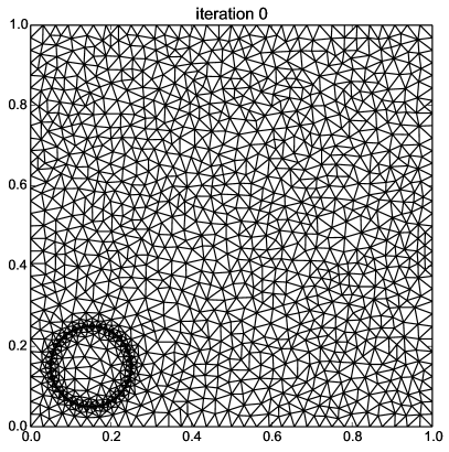
Figure 1: Inital mesh (left) and domain setup (right) with initial shape (bottom left) and optimal shape (top right).

In Figure 5, results of Algorithm 1 with the $H^{1}$ metric (left) and the Euclidean metric (right) are depicted. The gradient in the Euclidean metric is given by (cf. (3.34))

$$\nabla J^{h}(\Omega)=\sum_{k=1}^{2N}dJ^{h}_{vol}(\Omega)(v^{k})v^{k}$$ (5.4)

and the $H^{1}$ gradient is defined as the solution of the variational problem

$$(\nabla J^{h}(\Omega),\varphi)_{H^{1}}=dJ^{h}_{vol}(\Omega)(\varphi)\quad\text{ for all }\varphi\in\mathcal{V}_{N_{h}}(\mathcal{X},\mathbf{R}^{2}),$$ (5.5)

where the space $\mathcal{V}_{N_{h}}(\mathcal{X},\mathbf{R}^{2})$ is given by (3.40) with $\mathcal{X}=D$. The inital shape is now placed very close to the optimal shape and even overlaps it. The reason is that both gradient methods, the Euclidean and the $H^{1}$, are not able to perform large shape deformation and do do not converge when the inital shape is too far away. For the Euclidean metric to converge, the initial shape actually has to lie basically inside the optimal shape.

Opposite to this, it poses no problem for our novel variable metrics algorithm which proves to be much more robust in practise as demonstrated before. We also point out that the reconstructions in Figure 5 are not as good as the previous ones in Figure 2. The convergence history for the $H^{1}$ and the Euclidean metric based optimisations is depicted in Figure 4 (right).

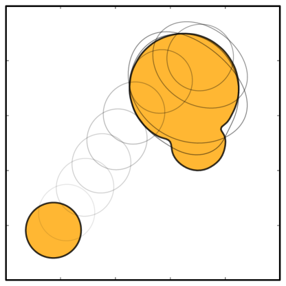
Figure 2: Shape progress for vvRKHS based optimisation with $\phi_{1}$ (left) and $\phi_{2}$ (right) for iterations 2, 5, 8, 11, 14, 17, 24, 30, 35, 50.

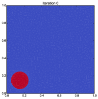
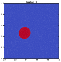
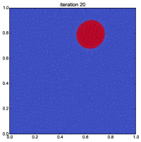
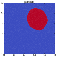
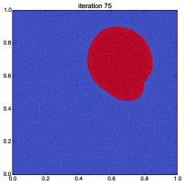
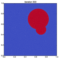
Figure 3: Successive meshes for iteration steps 0, 10, 20, 35, 55, 75, 120, 200, 500 of vvRKHS based optimisation with $\phi_{2}$.

Figure 4: Error progress for vvRKHS based iterations (left), $H^{1}$ and Euclidian metric (right).

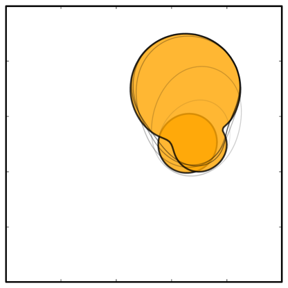
Figure 5: Shape progress for $H^{1}$ and Euclidian metric based optimisation.

Conclusion

We examined the applicability of RKHS in PDE constrained shape optimization. In particular, we showed that many previously used gradient algorithms can be identified as methods using gradients computed in RKHS. We also investigated special radial kernels and proposed a new variable metrics algorithm which exhibits very promising behaviour in our experimental setting. A comparison with other common methods shows that our method is much more robust when used with more complicated problems, namely when the distance to the optimal shape is large and its regularity is reduced (examine the non-convex areas). With the presented derivation and numerical demonstration of the new method, we only scratched the surface of this promising approach to shape optimisation in RKHS and many highly interesting question remain open. For instance, the “optimal choice” of the kernel for specific problems will be subject of future work.

References

• [1] L. Afraites, M. Dambrine, and D. Kateb. Shape methods for the transmission problem with a single measurement. Numer. Funct. Anal. Optim., 28(5-6):519–551, 2007.
• [2] G. Allaire, F. Jouve, and A.-M. Toader. A level-set method for shape optimization. C. R. Math. Acad. Sci. Paris, 334(12):1125–1130, 2002.
• [3] N. Aronszajn. Theory of reproducing kernels. Trans. Amer. Math. Soc., 68:337–404, 1950.
• [4] M. Berggren. A unified discrete-continuous sensitivity analysis method for shape optimization. In Applied and numerical partial differential equations, volume 15 of Comput. Methods Appl. Sci., pages 25–39. Springer, New York, 2010.
• [5] C. Carmeli, E. De Vito, and A. Toigo. Vector valued reproducing kernel Hilbert spaces of integrable functions and Mercer theorem. Anal. Appl. (Singap.), 4(4):377–408, 2006.
• [6] M. Delfour, G. Payre, and J.-P. Zolésio. An optimal triangulation for second-order elliptic problems. Comput. Methods Appl. Mech. Engrg., 50(3):231–261, 1985.
• [7] M. C. Delfour and J.-P. Zolésio. Shapes and geometries, volume 22 of Advances in Design and Control. Society for Industrial and Applied Mathematics (SIAM), Philadelphia, PA, second edition, 2011. Metrics, analysis, differential calculus, and optimization.
• [8] K. Eppler, H. Harbrecht, and R. Schneider. On convergence in elliptic shape optimization. SIAM J. Control Optim., 46(1):61–83 (electronic), 2007.
• [9] P. Gangl, U. Langer, A. Laurain, H. Meftahi, and K. Sturm. Shape Optimization of an Electric Motor Subject to Nonlinear Magnetostatics. SIAM J. Sci. Comput., 37(6):B1002–B1025, 2015.
• [10] A. Henrot and M. Pierre. Variation et optimisation de formes, volume 48 of Mathématiques & Applications (Berlin) [Mathematics & Applications]. Springer, Berlin, 2005. Une analyse géométrique. [A geometric analysis].
• [11] M. Hintermüller. Fast level-set based algorithms using shape and topological sensitivity information. Control and Cybernetics, 34(1):305–324, 2005.
• [12] R. Hiptmair, A. Paganini, and S. Sargheini. Comparison of approximate shape gradients. BIT, 55(2):459–485, 2015.
• [13] A. Laurain and Y. Privat. On a Bernoulli problem with geometric constraints. ESAIM Control Optim. Calc. Var., 18(1):157–180, 2012.
• [14] A. Laurain and K. Sturm. Distributed shape derivative via averaged adjoint method and applications. accepted for publication in ESAIM:M2AN, 2015.
• [15] P. W. Michor and D. Mumford. Riemannian geometries on spaces of plane curves. J. Eur. Math. Soc. (JEMS), 8(1):1–48, 2006.
• [16] S. Osher and R. Fedkiw. Level set methods and dynamic implicit surfaces, volume 153 of Applied Mathematical Sciences. Springer-Verlag, New York, 2003.
• [17] A. Paganini. Approximate shape gradients for interface problems. Technical Report 2014-12, Seminar for Applied Mathematics, ETH Zürich, Switzerland, 2014.
• [18] A. Paganini and R. Hiptmair. Approximate riesz representatives of shape gradients. Seminar for Applied Mathematics, ETH Zurich (Technical Report).
• [19] J. Sokołowski and J.-P. Zolésio. Introduction to shape optimization, volume 16 of Springer Series in Computational Mathematics. Springer-Verlag, Berlin, 1992. Shape sensitivity analysis.
• [20] K. Sturm. Minimax Lagrangian approach to the differentiability of nonlinear PDE constrained shape functions without saddle point assumption. SIAM J. Control Optim., 53(4):2017–2039, 2015.
• [21] K. Sturm. On shape optimization with non-linear partial differential equations. PhD thesis, Berlin, Technische Universität Berlin, Diss., 2015.
• [22] K. Sturm, D. Hömberg, and M. Hintermüller. Distortion compensation as a shape optimisation problem for a sharp interface model. Comp. Optim. and Appl., pages 1–32, 2016.
• [23] H. Wendland. Scattered data approximation, volume 17 of Cambridge Monographs on Applied and Computational Mathematics. Cambridge University Press, Cambridge, 2005.
• [24] L. Younes. Shapes and diffeomorphisms, volume 171 of Applied Mathematical Sciences. Springer-Verlag, Berlin, 2010.