On recovering missing values for sequences in a pathwise setting

Abstract

The paper suggests a frequency criterion of error-free recoverability of a missing value for sequences, i.e. discrete time processes, in a pathwise setting without probabilistic assumptions. The paper establishes error-free recoverability for classes of square-summable sequences with Z-transform vanishing with a mild rate at periodically located isolated points; the case of non-summable sequences is not excluded. The transfer functions for recovering algorithm are presented explicitly. Some robustness with respect to noise contamination is established for the suggested recovering algorithm.

Key words: data recovery, minimal Gaussian processes, pathwise criterions, frequency criterion, discrete time, Z-transform, robustness

I Introduction

A core problem of the mathematical theory of signal processing is the problem of recovery of missing data. For continuous data, the recoverability is associated with smoothness or analytical properties of the processes. For discrete time processes, it is less obvious how to interpret analyticity; so far, these problems were studied in a stochastic setting, where an observed process is deemed to be representative of an ensemble of paths with the probability distribution that is either known or can be estimated from repeating experiments. A classical result for stochastic stationary Gaussian processes with the spectral density $\phi$ is that a missing single value is recoverable with zero error if and only if

$$\int_{-\pi}^{\pi}\phi(\omega)^{-1}d\omega=-\infty.$$ (1)

(Kolmogorov [9], Theorem 24). Stochastic stationary Gaussian processes without this property are called minimal [9]. Criterion (1) was extended on stable processes Peller [16] and vector Gaussian processes Pourahmadi [17, 18]. Clearly, (1) holds for all “band-limited” processes meaning that the spectral density is vanishing on an arc of the unit circle ${\mathbb{T}}=\{z\in{\bf C}:\ |z|=1\}$.

It is known that signals with certain restrictions on the spectrum or sparsity feature recoverability of missing data in the pathwise setting without probabilistic assumptions. This setting targets situations where we deal with a sole sequence that is deemed to be unique and such that one cannot rely on statistics collected from observations of other similar samples. An estimate of the missing value has to be done based on the intrinsic properties of this sole sequence and the observed values. For example, a subsequence sampled at sparse enough periodic points can be removed from observations of an oversampling sequence [8]. In the compressive sensing setting, reducing of the sampling rate for finite sequences has been achieved using sparsity of signals [2, 3]. The connection of bandlimiteness and recoverability from samples was established for the fractional Fourier transform [15]. There is also a so-called Papoulis approach [14] allowing to reduce the sampling rate with additional measurements at sampling points; this approach was extended on multidimensional processes [1].

There is also an approach based on the so-called Landau’s phenomenon [10, 11];, it was shown in [10] that there is an uniqueness set of sampling points representing small deviations of integers for classes of functions with an arbitrarily large measure of the spectrum range. This result was extended on functions with unbounded spectrum range and on sampling points allowing a convenient explicit representation [12].

The paper suggests a criterion of error-free recoverability of sequences (discrete time processes) with spectrum degeneracy at isolated points similarly to (1). The result is based on the approach developed for pathwise predicting Dokuchaev [4, 5, 6], where some predictors were derived to establish error-free predictability. In the present paper, error-free recoverability is established for certain classes of square-summable sequences (processes) with Z-transform vanishing at a number of periodic isolated points (Theorem 1); the sequences are not necessarily summable. The required decay rate is mild; it can be selected as an arbitrarily low power of the distance to the nearest point of spectrum degeneracy. The corresponding recovering kernels are obtained and represented explicitly via their transfer functions. Some robustness with respect to noise contamination is established for the suggested recovering algorithm. A related result was obtained in [7]; however, the result obtained therein covers only the cases of sequences from $\ell_{1}$ with one-point spectrum degeneracy or sequences from $\ell_{2}$ that are band-limited, i.e. with Z-transform vanishing on an arc of the unit circle ${\mathbb{T}}$. It appears that the approach from D17 [7] is not applicable to processes $\ell_{2}\setminus\ell_{1}$ with spectrum degeneracy at isolated points, since the recovery kernels used therein were non-vanishing sequences from $\ell_{\infty}\setminus\ell_{2}$. The approach from D17 [7] requires additional restrains on the spectrum requiring a number of derivatives for Z-transform to vanish at a point. The approach of the present paper is quite different form the one from D17 [7] and does not involve restrictions on the derivatives of Z-transforms; instead, it focuses on underlying processes with spectrum vanishing at periodically located isolated points on ${\mathbb{T}}$.

II Some definitions and background

Let ${\mathbb{T}}\stackrel{{\scriptstyle{\scriptscriptstyle\Delta}}}{{=}}\{z\in{\bf C}:\ |z|=1\}$, and let ${\mathbb{Z}}$ be the set of all integers.

We denote by $\ell_{r}$ the set of all sequences $x=\{x(t)\}\subset{\bf C}$, $t=0,\pm 1,\pm 2,...$, such that $\|x\|_{\ell_{r}}=\left(\sum_{t=-\infty}^{\infty}|x(t)|^{r}\right)^{1/r}<+\infty$ for $r\in[1,\infty)$ or $\|x\|_{\ell_{\infty}}=\sup_{t}|x(t)|<+\infty$ for $r=+\infty$.

For $x\in\ell_{1}$ or $x\in\ell_{2}$, we denote by $X={\cal Z}x$ the Z-transform

$$X(z)=\sum_{t=-\infty}^{\infty}x(t)z^{-t},\quad z\in{\bf C}.$$

Respectively, the inverse $x={\cal Z}^{-1}X$ is defined as

$$x(t)=\frac{1}{2\pi}\int_{-\pi}^{\pi}X\left(e^{i\omega}\right)e^{i\omega t}d\omega,\quad t=0,\pm 1,\pm 2,....$$

We have that $x\in\ell_{2}$ if and only if $\|X\left(e^{i\omega}\right)\|_{L_{2}(-\pi,\pi)}<+\infty$. In addition, $\|x\|_{\ell_{\infty}}\leq\|X\left(e^{i\omega}\right)\|_{L_{1}(-\pi,\pi)}$.

We use the sign $\circ$ for convolution in $\ell_{2}$.

Let an integer $m\geq 0$ be given, let ${\cal T}_{m}=\{t\in{\mathbb{Z}}:\ |t|\leq m\}$, and let ${\cal T}_{2m}=\{t\in{\mathbb{Z}}:\ |t|\leq 2m\}$.

Let ${\cal H}$ be the set of all real sequences $h\in\ell_{2}$ such that $h(t)=0$ for $t\in{\cal T}_{2m}$.

The setting of recovery problem

We are interested in the problem of recovery values $\{x(r)\}_{r\in{\cal T}_{m}}$ from observations $\{x(s)\}_{s:\ |s|>m}$ for $x\in\ell_{2}$. More precisely, we consider calculation of estimates $\{\tilde{x}(r)\}_{r\in{\cal T}_{m}}$ obtained as $\widehat{x}=h\circ x$ for some appropriate kernels $h\in\ell_{2}$.

This recovery operator is time invariant and solves also the problem in the time invariant setting; for any $t\in{\mathbb{Z}}$, the values $\{x(t+r)\}_{r\in{\cal T}_{m}}$ will be estimated from observations $\{x(t+s)\}_{|s|>m}$ as $\{\tilde{x}(t+r)\}_{r\in{\cal T}_{m}}$.

Proposition 1 below shows that the recovery operators should be based on kernels $h\in{\cal H}$.

Proposition 1

1. If $x\in\ell_{2}$ and $h\in{\cal H}$, then, for any $r\in{\cal T}_{m}$,

   $$(h\circ x)(t+r)=\sum_{s\in{\mathbb{Z}}:\ |s-t|>m}h(t+r-s)x(s),$$ (2)

   i.e. the values $\{(h\circ x)(t+r)\}_{r\in{\cal T}_{m}}$ are calculated without use of $\{x(t+r)\}_{r\in{\cal T}_{m}}=\{x(s)\}_{s=t+r,\ |r|\geq m}$.

2. Let $h\in\ell_{2}$ be such that there exists $k\in{\cal T}_{2m}$ such that $h(k)\neq 0$, i.e. $h\notin{\cal H}$. Then for any $x\in\ell_{2}$ there exists $r\in{\cal T}_{m}$ such that $\xi\stackrel{{\scriptstyle{\scriptscriptstyle\Delta}}}{{=}}r-k\in{\cal T}_{m}$ and

   $$(h\circ x)(t+r)=h(k)x(t+\xi)$$

   $$+\sum_{s\in{\mathbb{Z}}:\ s\neq t+\xi}h(t+r-s)x(s).$$

In other words, the values $\{(h\circ x)(t+r)\}_{r\in{\cal T}_{m}}$ cannot be calculated without use of $\{x(s)\}_{s=t+r,\ |r|\leq m}$ under the assumptions of Proposition 1(ii).

Definition 1

Let ${\cal Y}\subset\ell_{2}$ be a class of sequences.

• We say that this class is recoverable if there exists a sequence $\{h_{n}(\cdot)\}_{n=1}^{+\infty}\subset{\cal H}$ and

  $$\sup_{t\in{\mathbb{Z}}}|x(t)-\widehat{x}_{n}(t)|\to 0\quad\hbox{as}\quad m\to+\infty\quad\forall x\in{\cal Y},$$

  where $\widehat{x}=h_{n}\circ x$.

• We say that the class ${\cal Y}$ is uniformly recoverable if, for any $\varepsilon>0$, there exists $h(\cdot)\in{\cal H}$ such that

  $$\sup_{t\in{\mathbb{Z}}}|x(t)-\widehat{x}(t)|\leq\varepsilon\quad\forall x\in{\cal Y},$$

  where $\widehat{x}=h\circ x$.

Since $h\circ x={\cal Z}(HX)$, where $H={\cal Z}h$ and $X={\cal Z}x$, then it follows that desired recovery operators should have the following properties.

• $h\in{\cal H}$;

• $H\left(e^{i\omega}\right)\cdot X\left(e^{i\omega}\right)\approx X\left(e^{i\omega}\right)$.

We will show below that this can be satisfied for appropriate choice of $h$ and for some wide enough classes of processes.

III The main results

We will establish recoverability for sequences with Z-transforms vanishing at some isolated points of ${\mathbb{T}}$ with certain rate.

Special classes of processes

Consider a continuous function $W:{\mathbb{T}}\setminus\{-1\}\to(0,+\infty)$ such that $\inf_{z\in{\mathbb{T}}\setminus\{-1\}}W(z)>0$ and that, for any $\varepsilon\in(0,\pi)$,

$$\int^{\pi}_{\varepsilon}W\left(e^{i\omega}\right)d\omega=+\infty.$$

Example III.1

One can select $W\left(e^{i\omega}\right)=(\pi-|\omega|)^{-1}$, $\omega\in(-\pi,\pi)$.

Let $M\stackrel{{\scriptstyle{\scriptscriptstyle\Delta}}}{{=}}2m+1$, i.e. $M$ is the number of elements in the set ${\cal T}_{m}$. Let

$$w(z)\stackrel{{\scriptstyle{\scriptscriptstyle\Delta}}}{{=}}W(z^{M}),\quad z\in{\mathbb{T}}.$$

Let ${\cal X}(w)$ be the class of all sequences $x\in\ell_{2}$ such that, for $X={\cal Z}x$,

$$\int_{-\pi}^{\pi}w\left(e^{i\omega}\right)|X\left(e^{i\omega}\right)|d\omega<+\infty.$$ (3)

Note that $w\left(e^{i\omega}\right)\to+\infty$ as $\omega\to\omega_{k}$, where

$$\omega_{k}=\frac{2\pi k-\pi}{M},\quad k\in{\cal T}_{2m}.$$

This means that (3) holds for “degenerate” processes, with $X\left(e^{i\omega}\right)$ vanishing as $\omega\to\omega_{k}$ with certain rate of decay defined by $w$. We call this $w$-degeneracy.

For $\omega,\widehat{\omega}\in(-\pi,\pi]$, let us define a ”distance”

$$d(\omega,\widehat{\omega})\stackrel{{\scriptstyle{\scriptscriptstyle\Delta}}}{{=}}\min(|\omega-\widehat{\omega}|,|\omega-(2\pi-\widehat{\omega})|).$$

Let

$$D_{\varepsilon}\stackrel{{\scriptstyle{\scriptscriptstyle\Delta}}}{{=}}\left\{\omega\in(-\pi,\pi]:\ \min_{k\in{\cal T}_{2m}}d(\omega,\omega_{k})\leq\varepsilon\right\}.$$

Example III.2

Let ${\cal X}^{\scriptscriptstyle BL}$ be the set of all $x\in\ell_{2}$ such that there exists $\varepsilon>0$ such that $X\left(e^{i\omega}\right)|_{\omega\in D_{\varepsilon}}=0$ (in particular, these processes are band-limited). Then ${\cal X}^{\scriptscriptstyle BL}\subset{\cal X}(w)$.

Definition 2

Let ${\cal U}(w)\subset{\cal X}(w)$ be a class of sequences. We say that this class features uniform $w$-degeneracy if, for any $x\in{\cal U}(w)$, for $X={\cal Z}x$,

$$\int_{D_{\varepsilon}}w\left(e^{i\omega}\right)|X\left(e^{i\omega}\right)|d\omega\to 0\quad\hbox{as}\quad\varepsilon\to 0+$$

$$\quad\hbox{uniformly over}\quad x\in{\cal U}(w).$$

Recovering kernels and recoverable sequences

Lemma 1

For $n>1$, consider kernels constructed as $h_{1}(\cdot)=h_{1,n}(\cdot)={\cal Z}^{-1}H_{n,1}$, where functions $H_{1,n}$ are such that

$$H\left(e^{i\omega}\right)=1,\quad |\omega|<\pi-1/n,$$

$$H_{1,n}\left(e^{i\omega}\right)=-W\left(e^{i\omega}\right),\quad |\omega|\in[\pi-1/n,\pi-\varepsilon_{n}],$$

$$H_{1,n}\left(e^{i\omega}\right)=0,\quad |\omega|\in(\pi-\varepsilon_{n},\pi).$$

Here $\varepsilon_{n}\in(0,1/n)$ are uniquely defined such that

$$\int^{\pi-\varepsilon_{n}}_{\pi-1/n}W\left(e^{i\omega}\right)d\omega=\pi-\frac{1}{n}.$$ (4)

Then $h_{1,n}\in\ell_{2}$ and $h_{1,n}(0)=0$.

Example III.3

For $W\left(e^{i\omega}\right)=(\pi-|\omega|)^{-1}$ from Example III.1, we have that $\varepsilon_{n}=e^{1/n-\pi}/n$. This can be calculated directly from matching

$$-\pi+1/n=\int^{\pi-\varepsilon_{n}}_{\pi-1/n}W\left(e^{i\omega}\right)d\omega=\ln(\pi-\omega)\bigl{|}_{\pi-1/n}^{\pi-\varepsilon_{n}}$$

$$=-\ln\varepsilon_{n}+\ln(1/n).$$

$\Box$

Lemma 2

Let $H_{M,n}(z)\stackrel{{\scriptstyle{\scriptscriptstyle\Delta}}}{{=}}H_{M,n}(z^{M})$, $z\in{\bf C}$. For $n>1$, consider kernels constructed as $h_{M,n}(\cdot)={\cal Z}^{-1}H_{M,n}$, where functions $H_{1,n}$ is defined in Lemma 1. Then $h_{M,n}\in\ell_{2}$ and $h_{M,n}(t)=0$ if $|t|\leq 2m$.

Since $H_{M,n}\left(e^{i\omega}\right)=1$ f on a large part of $(-\pi,\pi)$ for large $n\to+\infty$, the kernels introduced in Lemma 2 are potential candidates for the role of recovering kernels presented in Definition 1. The following theorem shows that these kernels ensure required recoverability for some classes of sequences.

Theorem 1

The following holds.

• The class ${\cal X}(w)$ is recoverable.

• Any class ${\cal U}(w)$ featuring uniform degeneracy in the sense of Definition 2 is uniformly recoverable.

• The kernels $h_{M,n}$ introduced in Lemma 2 ensure recovering required in (i) and (ii) as $n\to+\infty$. For these kernels,

  $$\sup_{t\in{\mathbb{Z}}}|x(t)-\widehat{x}(t)|\to 0\quad\hbox{as}\quad n\to+\infty\quad\forall x\in{\cal X}(w).$$

  Moreover, for any $\varepsilon>0$, there exists $n>0$ such that

  $$\sup_{t\in{\mathbb{Z}}}|x(t)-\widehat{x}(t)|\leq\varepsilon\quad\forall x\in{\cal U}(w).$$ (5)

  Here $\widehat{x}(t)\stackrel{{\scriptstyle{\scriptscriptstyle\Delta}}}{{=}}\sum_{s\in{\mathbb{Z}}}h_{M,n}(s)x(t-s).$

Some properties of predicting kernels

Let us outline some essential features of kernels $h_{n}$.

Clearly, $h_{M,n}(t)=h_{M,n}(-t)$ for all $t\in{\mathbb{Z}}$.

By the choice of $H_{1}$, it follows that $\sup_{n}\|H_{1,n}\left(e^{i\omega}\right)\|_{L_{1}(-\pi,\pi)}\leq 4\pi$ and $\sup_{n}\|h_{1,n}\|_{\ell_{2}}\leq 2$. Hence $\sup_{n}\|h_{M,n}\|_{\ell_{2}}\leq 2$.

Furthermore,Theorem 1 implies that one can decrease error by increasing $n$. On the other hand, we have that $\|H_{M,n}\left(e^{i\omega}\right)\|_{L_{2}(-\pi,\pi)}\to+\infty$ and hence $\|h_{M,n}\|_{\ell_{2}}\to+\infty$ as $n\to+\infty$. This means that the values $|h_{n}(t)|$ are decaying as $t\to+\infty$ slower for large $n$ required for lesser recovery error. Therefore, more precise recovery would be more impacted by data truncation and would require more observations, especially for heavy tail inputs.

On the case of fast decaying inputs from $\ell_{1}$

A related result based on different approach and different recovering kernels was obtained in in D17 [7] for sequences $x\in\ell_{1}$ such that $X\left(e^{i\omega}\right)$ is continuous in $\omega=\pi$ for $X={\cal Z}x$ together with $M-1$ derivatives in $\omega$ and such that $X\left(e^{i\omega}\right)$ vanishes at $\omega=\pi$ together with $M-1$ derivatives. Unfortunately, the corresponding kernels $h$ obtained therein were presented by non-decaying sequences from $\ell_{\infty}\setminus\ell_{2}$. It seems that the approach from D17 [7] is not applicable to processes $\ell_{2}\setminus\ell_{1}$. In particular, this cannot be resolved by truncation or dumping of the underlying input processes such as replacements of $x$ by $\{x(t)r^{-|t|}\}$ with $r>1$, since the spectrum degeneracy will not be preserved for the amended processes.

The approach of the present paper is quite different from the approach D17 [7]; in particular, it is based on different recovering kernels $h\in\ell_{2}$.

IV A numerical example

We made some numerical experiments with recovering kernels $h_{M,n}$ defined in Lemma 2 for $m=1$, $M=3$, and $W(\omega)=1/(\pi-|\omega|)$. As was mentioned above, these kernels are real valued even functions on ${\mathbb{Z}}$ such that $\|h_{M,n}\|_{\ell_{2}}\to+\infty$ as $n\to+\infty$. This means that, for large $n$, they may decay slow as $|t|\to+\infty$, which would lead to a large error caused by inevitable data truncation.

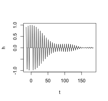
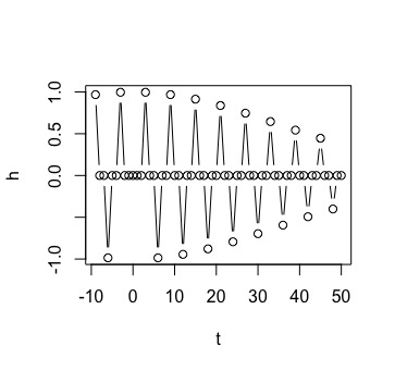
Figure 1: The kernel $h_{M,n}(t)$ for $m=1$, $M=3$, and $n=5$, for $t=0,1,...,200$ and $t=0,1,...,50$ (below).

Figure 1 show values of $h_{M,n}(t)$ for $m=1$, $M=2m+1=3$ and $n=5$.

We apply these kernel to an input processes $x\in{\cal H}$ obtained during each Monte-Carlo simulation as the following.

1. A Fourier polynomial $f_{1}(\omega)$ defined on $[-\pi,\pi]$ with $\bar{N}>0$ non-zero terms with independent random coefficients from normal distributions was created for a given $\bar{N}>0$.

2. A piecewise continuous function $f_{2}(\omega)=\sum_{\omega\in I_{k}}\alpha_{k}f_{1}(\omega)$ was created for random $\alpha_{k}=\xi_{k}+i\zeta_{k}$, where $\xi_{k}$ and $\zeta_{k}$ were selected independently from the normal distribution, and where $I_{k}=(-\pi+(k-1)\pi/\bar{N},-\pi+k\pi/\bar{N})$, $k=1,...,\bar{N}$.

3. We defined $X_{1}\left(e^{i\omega}\right)=f_{2}(\omega)+\overline{f_{2}(-\omega)}$. This would ensure that $X_{1}\left(e^{i\omega}\right)=\overline{X_{1}\left(e^{-i\omega}\right)}$, $\omega\in(-\pi,\pi]$.

4. A input process $x\in{\cal X}^{\scriptscriptstyle BL}$ was obtained using $X_{1}$ as $x={\cal Z}^{-1}\left({\mathbb{I}}_{\omega\in(-\pi,\pi]\setminus D_{\varepsilon}}X_{1}\left(e^{i\omega}\right)\right)$ for $\varepsilon\geq\varepsilon_{n}/3$. More precisely, a finite set of values for input process $\{x(t)\}_{t=-N}^{N}$ was calculated for a given $N>0$.

As was mentioned above, ${\cal X}^{\scriptscriptstyle BL}\subset{\cal X}(w)$ for any choice of $W$.

It can be noted that $n$ for the kernels $H_{M,n}$ and $\varepsilon$ for simulated $x$ were selected such that $\varepsilon>1/(3n)$, i.e., $n<1/(3\varepsilon)$; otherwise, the values (3) will be too large.

We have used R software; the command integrate was used for calculation of inverse Z-transforms for $h_{M,n}$ and $x$. We have used $\bar{N}=10$.

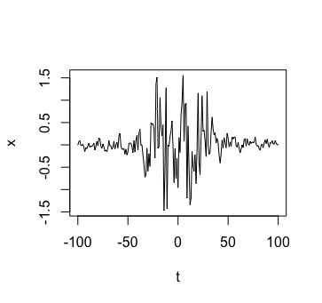
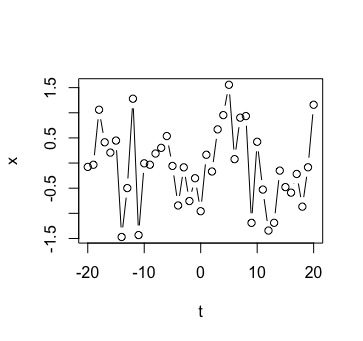
Figure 2: The path $x$ for $t=-300,...,300$ and for $t=-30,...,30$ (below) simulated with $\varepsilon=2/15$.

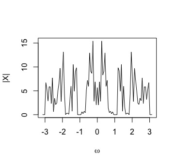
Figure 3: The trace of $|X\left(e^{i\omega}\right)|$ for the simulated path $x$ shown in Figure 2. It can be seen that the spectrum vanishes at the neighbourhood of points $\pi$ and $\pm\pi/3$.

Figure 2 shows an example of the path for $x$ simulated with $\varepsilon=2/9$ in two different scales. Figure 3 shows the trace $|X\left(e^{i\omega}\right)|$ for the corresponding $X={\cal Z}x$.

To test our algorithm for recovery of missing values $\{x(t)\}_{t=-1,0,1}$ from observations of $\{x(s)\}_{s:\,|s|\geq 2}$, we calculated their estimates $\widehat{x}(t)$ using convolution with the truncated input $x$

$$\widehat{x}(t)=\sum_{s\in{\mathbb{Z}}:\ |t-s|>1,|s|\leq N}h_{M,n}(t-s)x(s).$$

We calculated the relative error

$$E(N,n,\varepsilon)={\mathbb{E}}\frac{\sqrt{\frac{1}{3}\sum_{k=-1,0,1}|\widehat{x}(k)-x(k)|^{2}}}{\sqrt{\frac{1}{N}\sum_{t=-N}^{N}x(t)^{2}}}.$$

Here ${\mathbb{E}}$ means average over Monte-Carlo simulations. The following examples illustrate the impact of the choice of $N$, $n$, and $\varepsilon$, on the estimation error. In particular, we obtained that

• $E(150,3,1/9)=0.141$,  $E(150,3,2/9)=0.046$,

• $E(300,3,1/9)=0.060$, $E(300,3,2/9)=0.014$,

• $E(600,5,1/15)=0.039$,  $E(600,5,2/15)=0.001$.

These examples show that, as expected, the error is decreasing as the truncation parameter $N$ is increasing and as the measure of the spectrum gaps $\varepsilon$ is increasing.

V Proofs

Proof of Proposition 1. For $h\in{\cal H}$, we have that of $r\in{\cal T}_{m}$ that

$$(h\circ x)(t+r)=\sum_{s\in{\mathbb{Z}}:\ |t+r-s|>m}h(t+r-s)x(s).$$

If $|t+r-s|>2m$ then either $t+r-s>2m$ or $t+r-s<-2m$. Since $|r|\leq m$, then we have that either $t-s>2m-r\geq m$ or $t-s<-2m-r\leq-m$. In both cases, $|t-s|>m$. Hence (2) holds. This completes the proof of Proposition 1(i).

To prove Proposition 1(ii), it suffices to observe that there exists $r\in{\cal T}_{m}$ such that $\xi=r-k\in{\cal T}_{m}$. This completes the proof of Proposition 1. $\Box$

Proof of Lemma 1. Since $H_{1,n}\left(e^{-i\omega}\right)=\overline{H_{1,n}\left(e^{i\omega}\right)}$, we have that $h_{1,n}={\cal Z}^{-1}H_{1,n}$ is real valued. The choice of $W$ implies that there exists $\varepsilon_{n}\in(0,1/n)$ such that (4) holds. Further, (4) implies that

$$\int_{-\pi+\varepsilon_{n}}^{-\pi+1/n}H_{1,n}\left(e^{i\omega}\right)d\omega+\int^{\pi-\varepsilon_{n}}_{\pi-1/n}H_{1,n}\left(e^{i\omega}\right)d\omega$$

$$=2/n-2\pi=-\int_{-\pi+1/n}^{\pi-1/n}H_{1,n}\left(e^{i\omega}\right)d\omega.$$

Hence $\int_{-\pi}^{\pi}H_{1,n}\left(e^{i\omega}\right)d\omega=0$. Therefore,

$$h_{1,n}(0)=\frac{1}{2\pi}\int_{-\pi}^{\pi}H_{1,n}\left(e^{i\omega}\right)d\omega=0.$$

This completes the proof of Lemma 1. $\Box$

Proof of Lemma 2. It suffices to observe that $h_{M,n}(Mt)=h_{M,1}(t)$ and therefore $h_{M,n}(Mt)=0$ if $|t|\leq M-1=2m$. $\Box$

Proof of Theorem 1. Let $n\to+\infty$, and let $H=H_{M,n}$ be as defined above. Let $x\in{\cal X}(w)$, $X\stackrel{{\scriptstyle{\scriptscriptstyle\Delta}}}{{=}}{\cal Z}x$, $h={\cal Z}^{-1}H$, and

$$\widehat{x}(t)\stackrel{{\scriptstyle{\scriptscriptstyle\Delta}}}{{=}}\sum^{t}_{s=-\infty}h(t-s)x(s).$$

By the definitions, it follows that $\widehat{X}\left(e^{i\omega}\right)\stackrel{{\scriptstyle{\scriptscriptstyle\Delta}}}{{=}}H\left(e^{i\omega}\right)X\left(e^{i\omega}\right)=({\cal Z}\widehat{x})\left(e^{i\omega}\right)$.

We have that $\|\widehat{X}\left(e^{i\omega}\right)-X\left(e^{i\omega}\right)\|_{L_{1}(-\pi,\pi)}=I_{1}+I_{2}+I_{3},$ where

$$I_{k}=\int_{D_{k}}|\widehat{X}\left(e^{i\omega}\right)-X\left(e^{i\omega}\right)|d\omega$$

$$=\int_{D_{k}}|(H\left(e^{i\omega}\right)-1)X\left(e^{i\omega}\right)|d\omega,$$

and where $D_{k}=D_{k}(n)$, $k=1,2,3$, are defined as

$$D_{1}\stackrel{{\scriptstyle{\scriptscriptstyle\Delta}}}{{=}}(-\pi,\pi]\setminus(D_{2}\cup D_{3}),\quad$$

$$D_{2}\stackrel{{\scriptstyle{\scriptscriptstyle\Delta}}}{{=}}\cup_{k\in{\cal T}_{2m}}\left\{\omega\in(-\pi,\pi]:d(\omega,\omega_{k})\in\left[\frac{\varepsilon_{n}}{m},\frac{\pi}{mn}\right]\right\},\quad$$

$$D_{3}\stackrel{{\scriptstyle{\scriptscriptstyle\Delta}}}{{=}}\cup_{k\in{\cal T}_{2m}}\left\{\omega\in(-\pi,\pi]:d(\omega,\omega_{k})<\frac{\varepsilon_{n}}{m}\right\}.$$

By the choice of $H$ and $D_{1}$, it follows immediately that $I_{1}=0$.

Let us estimate $I_{2}$. We have that

$$I_{2}=\int_{D_{2}}|(H\left(e^{i\omega}\right)-1)X\left(e^{i\omega}\right)|d\omega\leq\zeta_{n}\psi_{n},$$

where

$$\zeta_{n}=\|w\left(e^{i\omega}\right)X\left(e^{i\omega}\right)\|_{L_{1}(D_{2})},\qquad$$

$$\psi_{n}=\left\|w\left(e^{i\omega}\right)^{-1}(H\left(e^{i\omega}\right)-1)\right\|_{L_{\infty}(D_{2})}.$$

We have that $w\left(e^{i\omega}\right)^{-1}H\left(e^{i\omega}\right)\equiv 1$ for $\omega\in D_{2}$. Hence $\sup_{n}\psi_{n}<+\infty$. By the assumptions on $X$,

$$\zeta_{n}\to 0\quad\hbox{as}\quad n\to+\infty.$$

Hence $I_{2}\to 0$ as $n\to+\infty$.

Let us estimate $I_{3}$. We have that

$$I_{3}=\int_{D_{3}}|(H\left(e^{i\omega}\right)-1)X\left(e^{i\omega}\right)|d\omega$$

$$=\int_{D_{3}}|X\left(e^{i\omega}\right)|d\omega\to 0\quad\hbox{as}\quad n\to+\infty.$$

It follows that $I_{1}+I_{2}+I_{3}\to 0$ for any $c>0$ and $x\in{\cal X}(w)$. Hence $\|\widehat{x}-x\|_{\ell_{\infty}}\to 0$ as $n\to+\infty$ for any $x\in{\cal X}(w)$. This completes the proof of statement (i).

Let us prove statement (ii). By the assumptions on ${\cal U}(w)$, it follows from the the proof above that

$$\|\widehat{X}\left(e^{i\omega}\right)-X\left(e^{i\omega}\right)\|_{L_{1}(-\pi,\pi)}=I_{1}+I_{2}+I_{3}$$

$$=I_{2}+I_{3}\to 0\quad\hbox{as}\quad n\to+\infty$$

uniformly over $x\in{\cal U}(w)$. In particular, for any $\varepsilon>0$, one can select $n$ such that $I_{2}+I_{3}\leq\varepsilon$, and this choice ensures that $\|\widehat{x}-x\|_{\ell_{\infty}}\leq\varepsilon$. This completes the proof of statement (ii). It follows from the proofs above that the recovering kernels $h(\cdot)={\cal Z}^{-1}H$ are such as required. This completes the proof of Theorem 1. $\Box$

VI On robustness with respect to noise contamination

Let us discuss the impact of the presence of the noise contaminating recoverable sequences. Assume that the kernels $h_{n}$ described in Theorem 1 and designed for recoverable sequences are applied to a sequence with a noise contamination. Let ${\cal U}(w)\subset{\cal X}$ be a set such as described in Definition 2. Let us consider an input sequence $x\in\ell_{2}$ such that $x=x_{0}+\eta$, where $x_{0}\in{\cal U}(w)$, and where $\eta\in\ell_{2}\setminus{\cal X}(w)$ represents a noise. Let $X={\cal Z}x$, $X_{0}={\cal Z}x_{0}$, and $N={\cal Z}\eta$. We assume that $\|N\left(e^{i\omega}\right)\|_{L_{1}(-\pi,\pi)}=\sigma$; the parameter $\sigma\geq 0$ represents the intensity of the noise.

In the proof of Theorem 1, we found that, for an arbitrarily small $\varepsilon>0$, there exists $n=n(p)$ such that

$$\int_{-\pi}^{\pi}|(H\left(e^{i\omega}\right)-1)X_{0}\left(e^{i\omega}\right)|d\omega\leq 2\pi\varepsilon\quad\forall x_{0}\in{\cal U}(w),$$

where $H={\cal Z}h$. For $\widehat{x}_{0}=h\circ x_{0}$, this implies that

$$\|\widehat{x}_{0}-x_{0}\|_{\ell_{\infty}}\leq\varepsilon.$$

Let us estimate the recovery error for the case where $\sigma>0$. For $\widehat{x}=h\circ x$, we have that

$$\|\widehat{x}-x\|_{\ell_{\infty}}\leq E_{0}+E_{\eta},$$

where

$$E_{0}=\frac{1}{2\pi}\|(H\left(e^{i\omega}\right)-1)X_{0}\left(e^{i\omega}\right)|\|_{L_{1}(-\pi,\pi)}\leq\varepsilon,\quad$$

$$E_{\eta}=\frac{1}{2\pi}\|(H\left(e^{i\omega}\right)-1)N\left(e^{i\omega}\right)|\|_{L_{1}(-\pi,\pi)}.$$

The value $E_{\eta}$ represents the additional error caused by the presence of unexpected high-frequency noise (when $\sigma>0$). It follows that

$$\|\widehat{x}-x\|_{\ell_{\infty}}\leq\varepsilon+\sigma(\kappa+1),$$ (6)

where $\kappa=\sup_{\omega\in[-\pi,\pi]}|H\left(e^{i\omega}\right)|$.

Therefore, it can be concluded that the recovering is robust with respect to noise contamination for any given $\varepsilon$.

It can be noted that if $\varepsilon\to 0$ then $n\to+\infty$ and $\kappa\to+\infty$. In this case, error (6) is increasing for any given $\sigma>0$. This happens when the recovering procedure is targeting too small a size of the error for the sequences from ${\cal X}(w)$, i.e., under the assumption that $\sigma=0$.

The equations describing the dependence of $\varepsilon$ and $\kappa$ on $n$ could be derived similarly to estimates in [5], Section 6 obtained for the predicting problem.

VII Discussion and future development

The paper suggests a frequency criterion of error-free recoverability of a finite set of missing values in pathwise deterministic setting in the spirit of the Kolmogorov’s criterion of minimality for stochastic Gaussian stationary processes Kolmogorov [9]. The paper suggests a robust recovering algorithm for classes of these sequences with periodic spectrum gaps.

Theorem 1 gives a criterion of recoverability that, for a special case where $M=1$, reminds the classical Kolmogorov’s criterion (1) of minimal recoverability formulated for the spectral densities Kolmogorov [9]. However, the degree of similarity is quite limited. For instance, if a stationary Gaussian process has the spectral density $\phi(\omega)\leq{\rm const\,}\cdot(\pi-|\omega|)$, $\omega\in(-\pi,\pi]$, then, according to criterion (1), this process is minimal Kolmogorov [9], i.e. a single missing value of this process is non-recoverable. On the other hand, Theorem 1 applied with $M=1$ and $W(\omega)=w\left(e^{i\omega}\right)=(\pi-|\omega|)^{-1}$ implies that the class ${\cal X}(w)$ is recoverable. In particular, this class includes all sequences $x\in\ell_{2}$ such that $|X\left(e^{i\omega}\right)|\leq{\rm const\,}\cdot(\pi-|\omega|)^{\alpha}$, where $X={\cal Z}x$ and $\omega\in(-\pi,\pi]$, and where $\alpha>0$ can be arbitrarily small. A similar example is given in D17 [7] for the case of summable processes from $\ell_{1}$. We leave this analysis for the future research.

There are other open questions. In particular, it is unclear if it is possible to obtain pathwise necessary conditions of recoverability in this pathwise setting based on Z-transform.

References

• [1] Cheung, K.F., Marks II. R.J. (1990). Imaging sampling below the Nyquist density without aliasing, J. Opt. Soc. Amer., vol. 7, no. 1, pp. 92-105, Jan. 1990.
• Donoho and Stark [1989] D. L. Donoho and P. B. Stark. (1989). Uncertainty principles and signal recovery. SIAM J. Appl. Math., vol. 49, no. 3, pp. 906–931.
• Candes et al [2006b] E.J. Candes, J. Romberg, T. Tao. (2006). Robust uncertainty principles: Exact signal reconstruction from highly incomplete frequency information. IEEE Transactions on Information Theory 52 (2), 489–509.
• Dokuchaev [2010a] N.Dokuchaev. (2012). On predictors for band-limited and high-frequency time series. Signal Processing 92, iss. 10, 2571-2575.
• Dokuchaev [2012b] N. Dokuchaev. (2012). Predictors for discrete time processes with energy decay on higher frequencies. IEEE Transactions on Signal Processing 60, No. 11, 6027-6030.
• Dokuchaev [2016] N. Dokuchaev. (2016). Near-ideal causal smoothing filters for the real sequences. Signal Processing 118, iss. 1, pp. 285-293.
• [7] Dokuchaev, N. (2017). On exact and optimal recovering of missing values for sequences. Signal Processing 135, 81–86. (ERA rating: A).
• [8] Ferreira P. G. S. G.. (1995). Sampling series with an infinite number of unknown samples. In: SampTA’95, 1995 Workshop on Sampling Theory and Applications, 268-271.
• Kolmogorov [1941] A.N. Kolmogorov. (1941). Interpolation and extrapolation of stationary stochastic series. Izv. Akad. Nauk SSSR Ser. Mat., 5:1, 3–14.
• [10] Landau H.J. (1964). A sparse regular sequence of exponentials closed on large sets. Bull. Amer. Math. Soc. 70, 566-569.
• [11] Landau H.J. (1967). Sampling, data transmission, and the Nyquist rate. Proc. IEEE 55 (10), 1701-1706.
• [12] Olevski, A., and Ulanovskii, A. (2008). Universal sampling and interpolation of band-limited signals. Geometric and Functional Analysis, vol. 18, no. 3, pp. 1029–1052.
• [13] Olevskii A.M. and Ulanovskii A. (2016). Functions with Disconnected Spectrum: Sampling, Interpolation, Translates. Amer. Math. Soc., Univ. Lect. Ser. Vol. 46.
• [14] Papoulis, A. (1977). Generalized Sampling Expansion, IEEE Trans. Circuits and Systems, v.24, 24(11), 652-654.
• [15] Wei, D. (2016) Super-resolution reconstruction using the high-order derivative interpolation associated with fractional filter functions, IET Signal Processing 10 (9), pp. 1052-1061.
• Peller [2000] V. V. Peller (2000). Regularity conditions for vectorial stationary processes. In: Complex Analysis, Operators, and Related Topics. The S.A. Vinogradov Memorial Volume. Ed. V. P. Khavin and N. K. Nikol’skii. Birkhauser Verlag, pp 287-301.
• Pourahmadi [1984] M. Pourahmadi (1984). On minimality and interpolation of harmonizable stable processes. SIAM Journal on Applied Mathematics, Vol. 44, No. 5, pp. 1023–1030.
• Pourahmadi [1989] M. Pourahmadi. Estimation and interpolation of missing values of a stationary time series. J. Time Ser. Anal., 10 (1989), pp. 149-169
• Tropp [2007] J. Tropp and A. Gilbert. (2007). Signal recovery from partial information via orthogonal matching pursuit, IEEE Trans. Inf. Theory, vol. 53, no. 12, pp. 4655–4666.
• [20] H. Zhao, R. Wang, D. Song, T. Zhang, D. Wu. (2014). Extrapolation of discrete bandlimited signals in linear canonical transform domain. Signal Processing 94, 212–218.
Refer to caption
Refer to caption