Identifying global optimality for dictionary learning

Abstract

Learning new representations of input observations in machine learning is often tackled using a factorization of the data. For many such problems, including sparse coding and matrix completion, learning these factorizations can be difficult, in terms of efficiency and to guarantee that the solution is a global minimum. Recently, a general class of objectives have been introduced—which we term induced dictionary learning models (DLMs)—that have an induced convex form that enables global optimization. Though attractive theoretically, this induced form is impractical, particularly for large or growing datasets. In this work, we investigate the use of practical alternating minimization algorithms for induced DLMs, that ensure convergence to global optima. We characterize the stationary points of these models, and, using these insights, highlight practical choices for the objectives. We then provide theoretical and empirical evidence that alternating minimization, from a random initialization, converges to global minima for a large subclass of induced DLMs. In particular, we take advantage of the existence of the (potentially unknown) convex induced form, to identify when stationary points are global minima for the dictionary learning objective. We then provide an empirical investigation into practical optimization choices for using alternating minimization for induced DLMs, for both batch and stochastic gradient descent.

Keywords: Matrix factorization, dictionary learning, sparse coding, alternating minimization, biconvex

1 Introduction

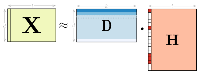
Figure 2: Sparse coding, with an overcomplete dictionary, $k>d$, and sparse re-representation. The red column in $\mathbf{H}$ corresponds to a high-dimensional, sparse re-representation of the first sample (column) in $\mathbf{X}$. The dictionary atoms (rows) in $\mathbf{D}$ intuitively correspond to prototypical examples.

Dictionary learning models (DLMs) are broadly used for unsupervised learning and representation learning, in the form of nonlinear dimensionality reduction, sparse coding, matrix completion and many matrix factorization-based approaches. The general form consists of factorizing an input matrix $\mathbf{X}$ into a dictionary $\mathbf{D}$ and a representation (or coefficients) $\mathbf{H}$, potentially transformed with a nonlinear transfer $f$: $\mathbf{X}\approx f(\mathbf{D}\mathbf{H})$ Singh and Gordon (2008); White (2014). Figure 1 depicts a common setting of obtaining a low-dimensional representation. As another example, shown in Figure 2, in sparse coding, the input observation $\mathbf{x}$ (a column of $\mathbf{X}$) is re-represented by sparse coefficients $\mathbf{h}$ (a column in $\mathbf{H}$), which linearly combines a small subset of dictionary elements (columns in $\mathbf{D}$). The motivation for sparse coding is based on mimicking the representation mechanism observed within the mammalian cortex Olshausen and Field (1997). In addition to this biological motivation, sparse coding has been demonstrated to be useful for image processing, with impressive denoising Elad and Aharon (2006) and classification results Raina et al. (2007); Mairal et al. (2009b); Jiang et al. (2011).

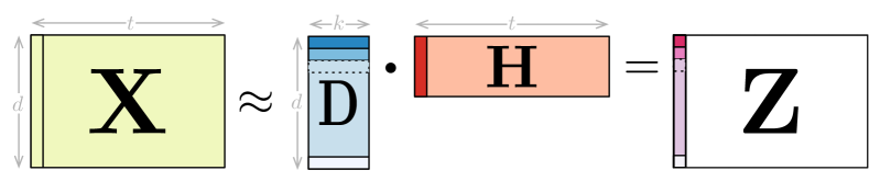
Figure 1: An example of the general form for Dictionary Learning Models (DLMs), where the inner dimension $k<d$, results in dimensionality reduction. The red column in $\mathbf{H}$ corresponds to a low-dimensional re-representation of the first sample (column) in $\mathbf{X}$. The dot product of the re-representation $\mathbf{H}$ with the dictionary $\mathbf{D}$ provides the approximation $\mathbf{Z}=\mathbf{D}\mathbf{H}$, where the dot product of the red column with $\mathbf{D}$ provides the first sample (column) in $\mathbf{Z}$ as the approximation to the first sample (column) in $\mathbf{X}$.

DLMs are attractive for unsupervised learning and representation learning, because in addition to their generality and simplicity, they are amenable to incremental estimation. Consequently, estimation can be performed on large datasets, and models can be updated with new data. These models are amenable to incremental estimation because only one of the variables—typically $\mathbf{H}$—grows with the number of samples. The other variable—typically $\mathbf{D}$—can be feasibly maintained incrementally, and sufficiently summarizes the solution. The ability to learn these models incrementally across samples additional provides the standard benefits from using stochastic gradient descent, including efficiency and being more reactive to non-stationary data. Despite these advantages, incremental estimation of DLMs has been under-explored.

The main reason for the restriction is the difficultly in optimal estimation of DLMs, even in the batch setting. The main difficultly arises from the fact that the optimization is over bilinear parameters $\mathbf{Z}=\mathbf{D}\mathbf{H}$, which interact to create a non-convex optimization. There have been impressive gains in recent years, in terms of obtaining optimal solutions to this non-convex problem. An important development has been the identification of induced DLMs: dictionary learning models that admit a convex regularizer directly on $\mathbf{Z}$, given the regularizers on $\mathbf{D}$ and $\mathbf{H}$. Consequently, by performing the optimization directly on $\mathbf{Z}$ instead of the factors, using the induced regularizer on $\mathbf{Z}$, the optimal solution can be obtained for the factor model. This insight has led to several convex reformulations, including for relaxed rank exponential family PCA Bach et al. (2008); Zhang et al. (2011), multi-view learning White et al. (2012), (semi-)supervised dictionary learning Goldberg et al. (2010); Zhang et al. (2011) and autoregressive moving average models White et al. (2015). This insight, however, is practically limited because the convex regularizer only has a known form for a small subset of induced DLMs and further the optimization is no longer amenable to incremental estimation because $\mathbf{Z}$ grows with the size of the data. Nonetheless, intuitively because this class enables convex reformulations, even though they are not computable, it identifies induced DLMs as a promising class to study to obtain global solutions for representation learning.

In that direction, there has been significant effort to understand the optimization surface of these non-convex objectives, including identifying that all local minima are global minima and proving that there are no deleterious saddlepoints (i.e., degenerate saddlepoints). There has been quite a bit work illustrating that alternating minimizations on the factors produces global models, including low-rank matrix completion with least-squares losses Mardani et al. (2013); Jain et al. (2013); Gunasekar et al. (2013), a thresholded sparse coding algorithm Agarwal et al. (2017, 2014), semi-definite low-rank optimization, where the two factors are the same $\mathbf{Z}=\mathbf{D}\mathbf{D}^{\top}$ d’Aspremont et al. (2004); Burer and Monteiro (2005); Bach et al. (2008); Journée et al. (2010); Zhang et al. (2012); Mirzazadeh et al. (2015) and for a generalized factorization setting that includes (rectified) linear neural networks Haeffele and Vidal (2015); Kawaguchi (2016). These approaches provide important seminal results, but still only characterize a small subset of induced DLMs, particularly requiring rank-deficient (i.e., low rank) solutions or specialized initialization strategies.

For incremental estimation, the guarantees become further limited. There are specialized incremental algorithms for principal components analysis Warmuth and Kuzmin (2008); Feng et al. (2013) and partial least-squares Arora et al. (2012). Results characterizing the optimization surface Haeffele and Vidal (2015) provide insights on the optimality of stochastic gradient descent; however, as mentioned, such characterizations have been largely limited to rank-deficient solutions. For other settings, little is known about how to obtain optimal incremental DLM  estimation and, particularly for incremental sparse coding, several approaches have settled for local solutions Mairal et al. (2009a, b, 2010). Yet, as we argue, there is more room to take advantage of the induced form for these models, to identify and theoretically characterize tractable objectives.

In this work, we provide both theoretical and empirical evidence that gradient descent on the non-convex, factored form for induced DLMs produces global solutions for a broad class of induced DLMs. We make the following conjecture, that leads to simple and effective global optimization algorithms for induced DLMs.

Alternating minimization for induced dictionary learning models, with a full rank random initialization, converges to a globally optimal solution.

The key contributions of this paper are to provide evidence for this conjecture and to develop effective optimization techniques based on alternating minimization. We first expand the set of induced DLMs, and propose several practical modifications to previous objectives, particularly to enable incremental estimation. We prove a novel result that a large subclass of induced DLMs satisfy the property that every local minimum is a global minimum, and further demonstrate that a subclass does not have degenerate saddle-points, providing compelling evidence that alternating minimization will successfully find global minima. The key novelty in our theoretical results is a new approach to characterizing the overcomplete setting, for full rank solutions $\mathbf{D},\mathbf{H}$, as opposed to the more studied rank-deficient setting. We provide empirical support for the above conjecture, in particular illustrating that small deviations to outside the class of induced DLMs no longer have the property that alternating minimization produces global solutions. With this justification for alternating minimization, we then develop algorithms that converge faster than vanilla implementations of alternating minimization, for both batch and stochastic gradient descent.

In addition to providing evidence for this conjecture, the theoretical results in this work provide a new methodology for analyzing stationary points for general dictionary learning problems. With analysis conducted under this more general class of models, we automatically obtain novel results for specific settings of interest, including matrix completion, sparse coding and dictionary learning with elastic net regularization. The current assumptions require differentiability, which restricts the results to smooth versions of these problems. Nonetheless, it provides first steps towards a unified analysis that, with extensions to non-smooth functions, could address many of these settings simultaneously.

The paper is organized as follows. We first motivate the types of dictionary learning problems that can be specified as induced DLMs (Section 2) and then discuss how to generalize and improve these objectives (Section 3). Then we prove the main theoretical result (Section 4) and further provide empirical evidence for the conjecture (Section 5), highlighting some practical optimization choices for the batch setting. We then propose several incremental algorithms to optimize induced DLMs, to make it feasible to learn these models for large datasets (Section 6). Finally, we summarize a large body of related work (Section 7) and conclude with a discussion on current limitations of this work and important next steps.

2 Dictionary Learning Models

In this section, we introduce induced DLMs and provide several examples of objectives that are within the class. We focus on examples that demonstrate how this optimization formalism can be used to obtain different representation properties as well as more modern uses to help unify recently introduced models under the formalism. Suitable objectives for these models are summarized in Table 1, which include subspace dictionary learning, matrix completion, sparse coding and elastic-net dictionary learning. See (White, 2014, Section 3.4) for a more complete overview of the representational capabilities of the larger class of DLMs. The goal of this section is to provide intuition for the uses and generality of induced DLMs.

We begin by defining the class of induced DLMs. Let $\mathbf{X}\in\mathbb{R}^{n\times T}$ consist of $T$ samples of $n$ features. The goal is to learn a bilinear factorization $\mathbf{Z}=\mathbf{D}\mathbf{H}$ where $\mathbf{D}\in\mathbb{R}^{d\times k}$ and $\mathbf{H}\in\mathbb{R}^{k\times T}$ for given $d,k$, given any convex loss $\mathrm{L}:\mathbb{R}^{d\times T}\rightarrow\mathbb{R}$. For example, the loss could be the sum of squared errors between the reconstruction and the input,

$$\mathrm{L}(\mathbf{Z},\mathbf{X})=\sum_{t=1}^{T}L_{x}(\mathbf{Z}_{:t},\mathbf{X}_{:t})\hskip 28.45274pt\text{ for }\ \ \ L_{x}(\mathbf{Z}_{:t},\mathbf{X}_{:t})=\|\mathbf{Z}_{:t}-\mathbf{X}_{:t}\|_{2}^{2}.$$

More generally, this convex loss will typically be defined based on a transfer (or activation function) $f:\mathbb{R}\rightarrow\mathbb{R}$ and the corresponding matching loss $L_{x}(\mathbf{Z}_{:t},\mathbf{X}_{:t})$ that is convex in the first argument (see Helmbold et al. (1996)). This loss evaluates the difference between $f(\mathbf{Z}_{:t})$ and $\mathbf{X}_{:t}$, with overloaded definition that $f(\mathbf{Z}_{:t})$ or $f(\mathbf{Z})$ is the transfer $f$ applied to each entry of the input vector or matrix. For example, $f$ could be an identity function, resulting in no transformation, and $L_{x}(\mathbf{Z}_{:t},\mathbf{X}_{:t})=\|\mathbf{Z}_{:t}-\mathbf{X}_{:t}\|_{2}^{2}$. As another example, $f$ could be the sigmoid function and $L_{x}(\mathbf{Z}_{:t},\mathbf{X}_{:t})$ the cross-entropy.

Additionally, the DLM objective is characterized by the choice of regularizers. Properties on $\mathbf{D}$ and $\mathbf{H}$ are encoded using convex regularizers ${\mathrm{R}_{\mathrm{\scriptsize D}}}:\mathbb{R}^{d\times k}\rightarrow\mathbb{R}$ and ${\mathrm{R}_{\mathrm{\scriptsize H}}}:\mathbb{R}^{k\times T}\rightarrow\mathbb{R}$. As we describe in the cases studies in the remainder of this section, common choices for these regularizers are $\ell_{2}$ norms—for low-rank solutions—and $\ell_{1}$ norms—for sparse solutions.

The general optimization for FMs corresponds to

$$\min_{\mathbf{D}\in\mathbb{R}^{d\times k},\ \mathbf{H}\in\mathbb{R}^{k\times T}}\mathrm{L}(\mathbf{D}\mathbf{H})+{\mathrm{R}_{\mathrm{\scriptsize D}}}(\mathbf{D})+{\mathrm{R}_{\mathrm{\scriptsize H}}}(\mathbf{H})$$ (1)

Induced DLMs correspond to a subclass of this more general objective, where there are additional conditions on these regularizers. The condition is that there is a convex induced regularizer ${\mathrm{R}_{\mathrm{\scriptsize Z}}}$ on the product $\mathbf{Z}=\mathbf{D}\mathbf{H}$, that satisfies

$${\mathrm{R}_{\mathrm{\scriptsize Z}}}(\mathbf{Z})=\frac{1}{2}\min_{\begin{subarray}{c}\mathbf{D}\in\mathbb{R}^{d\times k},\ \mathbf{H}\in\mathbb{R}^{k\times T}\\ \mathbf{Z}=\mathbf{D}\mathbf{H}\end{subarray}}{\mathrm{R}_{\mathrm{\scriptsize D}}}(\mathbf{D})+{\mathrm{R}_{\mathrm{\scriptsize H}}}(\mathbf{H}).$$ (2)

This property is potentially useful because the resulting optimization over $\mathbf{Z}$ is convex, providing a convex reformulation of the non-convex DLM objective. This reformulation has been extensively used for learning lower-dimensional representations, with the trace norm (aka nuclear norm). Further, Bach et al. (2008) proved that, if $k$ is sufficiently large (potentially infinite), then there exists an induced regularizer when

$${\mathrm{R}_{\mathrm{\scriptsize D}}}(\mathbf{D}) =\alpha\sum_{i=1}^{k}\|\mathbf{D}_{:,i}\|^{2}_{c}$$

$${\mathrm{R}_{\mathrm{\scriptsize H}}}(\mathbf{H}) =\alpha\sum_{i=1}^{k}\|\mathbf{H}_{i,:}\|^{2}_{r}$$

for column and row norm regularizers $\|\cdot\|_{c}$ and $\|\cdot\|_{r}$, with regularization parameter $\alpha\geq 0$. This result was further generalized by Haeffele and Vidal (2015) and we provide a further generalization in Proposition 1.

The direct use of this convex reformulation, however, is limited for two reasons. First, an explicit form for the induced regularizer ${\mathrm{R}_{\mathrm{\scriptsize Z}}}$ is only known for a small number of settings. Second, only for a further subset of these, is there a clear way to extract the corresponding optimal $\mathbf{D},\mathbf{H}$ from the learned $\mathbf{Z}=\mathbf{D}\mathbf{H}$. Intuitively, however, this property identifies a class of well-behaved problems. We will show that it is preferable to directly learn $\mathbf{D},\mathbf{H}$, with a simple gradient descent approach on the non-convex factored objective, and simply use the existence of this convex reformulation to identify promising, tractable objectives.

Given this general definition of induced DLMs, we now turn to providing more specific examples. For each of the examples of induced DLMs, we will highlight if they have a known induced regularizer. The purpose of this summary is to unify existing representation learning approaches under induced DLMs, as well as provide examples of how to encode properties on the learned representation $\mathbf{H}$ using the relatively simple induced DLM  formalism.

2.1 Subspace dictionary learning, including nonlinear dimensionality reduction

A common goal in representation learning is to to obtain a lower-dimensional representation of input $\mathbf{X}$. Learning such a low-dimensional representation using an induced DLM  objective has typically been formulated (Bach et al., 2008; Zhang et al., 2011) by setting $\|\cdot\|_{c}=\|\cdot\|_{2}=\|\cdot\|_{r}$, and $\mathrm{L}(\mathbf{Z})=\sum_{t=1}^{T}L_{x}(\mathbf{Z}_{:t},\mathbf{X}_{:t})$. The corresponding induced convex reformulation is

$$\min_{\mathbf{D}\in\mathbb{R}^{d\times k},\mathbf{H}\in\mathbb{R}^{k\times T}} \mathrm{L}(\mathbf{D}\mathbf{H})+\tfrac{\alpha}{2}\left\|\mathbf{D}\right\|_{F}^{2}+\tfrac{\alpha}{2}\left\|\mathbf{H}\right\|_{F}^{2}$$ (3)

$$=\min_{\mathbf{Z}\in\mathbb{R}^{d\times T}}\mathrm{L}(\mathbf{Z})+\alpha\left\|\mathbf{Z}\right\|_{tr}\ \ \ \ \ \ \ \triangleright\text{ if }k\geq d$$ (4)

where the Frobenius norm is defined as $\|\mathbf{D}\|_{F}^{2}=\sum_{i=1}^{k}\|\mathbf{D}_{:,i}\|_{2}^{2}$ and the trace norm (or nuclear norm) is defined as $\left\|\mathbf{Z}\right\|_{tr}=\sum_{i=1}^{\min(d,T)}\sigma_{i}(\mathbf{Z})$. This objective corresponds to a relaxed rank formulation of principal components analysis (PCA). To obtain the standard PCA objective Xu et al. (2009), $\alpha$ is set to zero and $k<d$ is set to the desired rank, with $L_{x}(\mathbf{Z}_{:t},\mathbf{X}_{:t})=\left\|\mathbf{Z}_{:t}-\mathbf{X}_{:t}\right\|_{F}^{2}$. The resulting $\mathbf{Z}$ corresponds to a low rank approximation to $\mathbf{X}$, that consists of the top $k$ singular values and vectors of $\mathbf{X}$: given singular value decomposition $\mathbf{X}=\mathbf{U}\bm{\Sigma}\mathbf{V}^{\top}$, the resulting $\mathbf{Z}=\mathbf{U}\bm{\Sigma}_{k}\mathbf{V}^{\top}$ where $\bm{\Sigma}_{k}$ is a diagonal matrix of the top $k$ singular values of $\bm{\Sigma}$ and the rest set to zero. For the relaxed rank setting, with $\alpha>0$, the optimal solution is $\mathbf{Z}=\mathbf{U}(\bm{\Sigma}-\alpha)_{+}\mathbf{V}^{\top}$, where $(\cdot)_{+}$ truncates negative values at zero. For this case, instead of fixing $k$ to a smaller rank, the rank is implicitly restricted by the induced regularizer on $\mathbf{Z}$, and for the factored form, by the regularizers on $\mathbf{D}$ and $\mathbf{H}$.

To further understand why these chosen column and row norms result in this dimensionality reduction effect, consider the induced norm. The trace norm is known to be a tight convex relaxation of rank. The optimization over $\mathbf{Z}$, for large enough $\alpha$, selects a lower rank $\mathbf{Z}=\mathbf{D}\mathbf{H}=\mathbf{U}(\bm{\Sigma}-\alpha)_{+}\mathbf{V}^{\top}$ as described. Further, it is well known that the above formulation can be equivalently written as a constrained form with a $(2,1)$-block norm on $\mathbf{H}$:

$$\min_{\mathbf{D}\in\mathbb{R}^{d\times k},\mathbf{H}\in\mathbb{R}^{k\times T}} \mathrm{L}(\mathbf{D}\mathbf{H})+\tfrac{\alpha}{2}\left\|\mathbf{D}\right\|_{F}^{2}+\tfrac{\alpha}{2}\left\|\mathbf{H}\right\|_{F}^{2} =\min_{\begin{subarray}{c}\mathbf{H}\in\mathbb{R}^{k\times T},\mathbf{D}\in\mathbb{R}^{d\times k}\\ \|\mathbf{D}_{:i}\|_{2}\leq 1\end{subarray}}\mathrm{L}(\mathbf{D}\mathbf{H})+\alpha\sum_{i=1}^{k}\|\mathbf{H}_{i:}\|_{2}$$

The $(2,1)$-block norm constitutes a group-sparse regularizer on $\mathbf{H}$, where the sum of the $\ell_{2}$ norms encourages entire rows of $\mathbf{H}$ to be zero Argyriou et al. (2008); White (2014). Once an entire row of $\mathbf{H}$ is set to zero, the rank is reduced by one, and the implicit $k$ is actually one less.

These subspace dictionary learning objectives encompass a wide-range of dimensionality reduction approaches, including principal components analysis, canonical correlation analysis, partial least-squares and nonlinear dimensionality reduction approaches such as Isomap and non-linear embeddings White (2014). To obtain non-linear dimensionality reduction, the inputs $\mathbf{x}$ are first transformed with kernels, and then the same subspace dictionary learning optimization used above. Similarly to PCA, we can additionally obtain relaxed rank versions of each of these nonlinear dimensionality approaches.

2.2 Matrix completion

The matrix completion problem, formulated as a low-rank completion problem Candes and Recht (2009), is an instance of subspace dictionary learning. The matrix completion problem is often used for collaborative filtering, where the goal is to infer rankings or information about a user using a small amount of labeled information from other users. For example, for Netflix ratings, the goal is to complete a matrix of ratings, with $d$ users as rows and $T$ movies as columns. Each $\mathbf{X}_{ij}$ corresponds to a rating for user $i$ and movie $j$, where only a subset of such ratings will be available. The idea behind finding a low-rank $\mathbf{D}$ and $\mathbf{H}$ to factorize the known components of $\mathbf{X}$ is that there is some latent structure that explains the ratings.

A common objective for matrix completion is

$$\sum_{\text{observed }(i,j)}(\mathbf{X}_{ij}-\mathbf{D}_{i:}\mathbf{H}_{:j})^{2}+\alpha\left\|\mathbf{D}\right\|_{F}^{2}+\alpha\left\|\mathbf{H}\right\|_{F}^{2}$$

which is an instance of the subspace objective in (3). There are numerous variations on this basic objective to improve performance. For example, Salakhutdinov and Srebro (2010) use weighted norms for non-uniform sampling, giving

$$\sum_{\text{observed }(i,j)}(\mathbf{X}_{ij}-\mathbf{D}_{i:}\mathbf{H}_{:j})^{2}+\alpha\left\|\bm{\Lambda}_{D}\mathbf{D}\right\|_{F}^{2}+\alpha\left\|\mathbf{H}\bm{\Lambda}_{H}\right\|_{F}^{2}$$

where $\bm{\Lambda}_{D}\in\mathbb{R}^{d\times d}$ is a positive diagonal matrix that reweights rows of $\mathbf{D}$ and where $\bm{\Lambda}_{H}\in\mathbb{R}^{T\times T}$ is a positive diagonal matrix that reweights columns of $\mathbf{H}$. With a change of variables, this can equivalently be written as a minimization over

$$\sum_{\text{observed }(i,j)}(\mathbf{X}_{ij}-\bm{\Lambda}_{D}(i,i)^{-1}\bm{\Lambda}_{H}(j,j)^{-1}\mathbf{D}_{i:}\mathbf{H}_{:j})^{2}+\alpha\left\|\mathbf{D}\right\|_{F}^{2}+\alpha\left\|\mathbf{H}\right\|_{F}^{2}$$

where

$$\mathrm{L}(\mathbf{D}\mathbf{H}) =\sum_{\text{observed }(i,j)}(\mathbf{X}_{ij}-\bm{\Lambda}_{D}(i,i)^{-1}\bm{\Lambda}_{H}(j,j)^{-1}(\mathbf{D}\mathbf{H})_{ij})^{2}$$

$$=\sum_{\text{observed }(i,j)}(\mathbf{X}_{ij}-\bm{\Lambda}_{D}(i,i)^{-1}\bm{\Lambda}_{H}(j,j)^{-1}\mathbf{D}_{i:}\mathbf{H}_{:j})^{2}.$$

As with subspace learning, $k$ is set less than $d$, and $\alpha$ is tuned to obtain a lower-dimensional $\mathbf{D},\mathbf{H}$. Each user has $k$ explanatory variables, where the column $\mathbf{D}_{:l}$ corresponds to the value of that variable for all the users and $\mathbf{H}_{l:}$ corresponds to the value for that variable for all the movies. Though these latent variables may have no interpreation, intuitively one could imagine that they describe general properties of users and movies. For example, column $l$ in $\mathbf{D}$ could correspond to “likes romance” and the corresponding row in $\mathbf{H}$ could be “movie has romance”. The dot product $\mathbf{X}_{ij}=\mathbf{D}_{i:}\mathbf{H}_{:j}$ would include $\mathbf{D}_{il}\mathbf{H}_{lj}$. If the user does not like romance, or the movie does not have romance, these coefficients might be zero and will not contribute to the dot product; else, if the movie has romance and the user likes romance, the coefficients are likely non-negligible and can be predictive of a high rating. Even though $\mathbf{X}_{ij}$ is only know for a small subset of $\mathbf{X}$, we learn the properties $\mathbf{D}_{:l}$ and $\mathbf{H}_{l:}$ for all users and movies based on the information that is available. Once we learn these properties, we can complete the unknown ratings using $\mathbf{X}_{ij}=\mathbf{D}_{i:}\mathbf{H}_{:j}$.

2.3 Sparse coding

The aim in sparse coding is to re-represent the inputs with a sparse set of coefficients, that linearly weight a subset of representative dictionary atoms (columns of $\mathbf{D}$). Sparse coding was originally introduced based on observed representations in the mammalian brain (Olshausen and Field, 1997), and has since proven practically useful particularly in image processing, where dictionary atoms can encode edges and other modular components within images. A similar such premise underlies many representations. Consider an extreme form of sparse coding, where only one element in $\mathbf{H}_{:j}$ is active; this represents an indicator to the bin for the given input, and can be thought of as clustering or aggregation. Sparse coding can be seen as selecting a small number of key properties to re-represent the input; similar inputs should have similar—or at least overlapping—active properties.

A sparse representation is typically obtained by using an $\ell_{1}$ norm on $\mathbf{H}$, with induced DLM objective

$$\min_{\mathbf{D}\in\mathbb{R}^{d\times k},\mathbf{H}\in\mathbb{R}^{k\times T}}\mathrm{L}(\mathbf{D}\mathbf{H})+\tfrac{\alpha}{2}\sum_{i=1}^{k}\|\mathbf{D}_{:,i}\|^{2}_{q}+\tfrac{\alpha}{2}\sum_{i=1}^{k}\|\mathbf{H}_{i,:}\|^{2}_{1}.$$ (5)

where $\|\mathbf{Z}^{\top}\|_{q,1}=\sum_{i}\|\mathbf{Z}_{:,i}\|_{q}$ can have any $q\geq 1$. This objective has a known convex induced regularizer (Zhang et al., 2011, Proposition 2)), as long as $k\geq T$

$$\eqref{eq_sparseobj}=\min_{\mathbf{Z}\in\mathbb{R}^{d\times T}}\mathrm{L}(\mathbf{Z})+\alpha\|\mathbf{Z}^{\top}\|_{q,1}\ \ \ \ \ \ \ \triangleright\text{ if }k\geq T.$$

The resulting global solution, however, requires $k=T$ and corresponds to memorizing normalized observations: $\mathbf{D}_{:,i}=\mathbf{Z}_{:,i}/\|\mathbf{Z}_{:,i}\|_{q}$ and diagonal $\mathbf{H}_{i,i}=\|\mathbf{Z}_{:,i}\|_{q}$. To remedy this issue with induced DLMs and sparse learning, Bach et al. (2008) proposed to combine the subspace and sparse regularizers, described in the next subsection. In this work, we highlight that this objective may actually have a convex induced regularizer for smaller $k$, even though the form of this induced regularizer may not be known.

2.4 Elastic-net dictionary learning

We can interpolate between both subspace and sparse regularizers (also called elastic net regularization Zou and Hastie (2005)), using parameters $\nu_{\textrm{D}},\nu_{\textrm{H}}\in[0,1]$

$$\min_{\mathbf{D}\in\mathbb{R}^{d\times k},\mathbf{H}\in\mathbb{R}^{k\times T}}\mathrm{L}(\mathbf{D}\mathbf{H})+\tfrac{\alpha}{2}\sum_{i=1}^{k}\Big{[}\nu_{\textrm{D}}\|\mathbf{D}_{:i}\|_{2}^{2}+(1-\nu_{\textrm{D}})\|\mathbf{D}_{:,i}\|^{2}_{1}+\nu_{\textrm{H}}\|\mathbf{H}_{i:}\|_{2}^{2}+(1-\nu_{\textrm{H}})\|\mathbf{H}_{i,:}\|^{2}_{1}\Big{]}$$

with elastic net norm $\|\mathbf{v}\|=\sqrt{\nu\|\mathbf{v}\|_{2}^{2}+(1-\nu)\|\mathbf{v}\|_{1}^{2}}$. This regularizer should prefer a more compact sparse representation $\mathbf{H}$. Previous results indicate improved stability and compactness Zou and Hastie (2005); we verify these properties for representation learning in Section 6, showing that $k$ can be smaller with the elastic net objective compared to the sparse coding objective.

The elastic-net objective is an instance of an induced DLM, because the elastic net norm is a valid column and row norm (see Proposition 12 in Appendix A) and so we know that a corresponding induced norm on $\mathbf{Z}$ exists for sufficiently large $k$. However, unlike the previously described induced DLMs, there is no known efficiently computable form for the induced regularizer. For this reason, this regularizer remains one of the bigger open questions for induced DLMs. It is additionally a motivator for using the existence of the induced regularizer, without requiring a known form.

Though we write the above having the elastic net norm on both factors, this is not necessary. An elastic net norm could be used on one factor, and a completely different norm on another factor. We simply write the above to introduce notation, and because several common settings are obtained with different $\nu_{\textrm{D}}$ and $\nu_{\textrm{H}}$. For example, for $\nu_{\textrm{D}}=1$, we have an $\ell_{2}$ regularizer on the columns of $\mathbf{D}$, and an elastic net norm on the rows of $\mathbf{H}$, which is the setting addressed by Bach et al. (2008).

2.5 Supervised dictionary learning

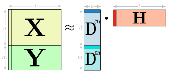
Figure 3: Supervised dictionary learning, with a separate dictionary for the input $\mathbf{X}$ and the target $\mathbf{Y}$. This example depicts $k<d$, giving dimensionality reduction, though other choices such as a higher-dimensional, sparse representation could have also been used.

The objectives so far have focused on unsupervised learning; however, for many cases, the goal is to improve supervised learning, which can be elegantly incorporated under DLMs. A typical strategy is to learn a new representation in an unsupervised way, and then use that representation to learn a supervised predictor given labeled samples. These two stages can be combined into one objective, where the new factorized representation is learned for $\mathbf{X}$ while also using it for supervised learning, given some labels $\mathbf{Y}\in\mathbb{R}^{m\times T}$. For simplicity we will assume that we have labels corresponding to each sample (column) in $\mathbf{X}$; this can be relaxed to a semi-supervised setting by ignoring missing entries in the supervised loss component Zhang et al. (2011).

The supervised DLM  is (Goldberg et al., 2010; Zhang et al., 2011; White et al., 2012)

$$\mathop{\mathrm{argmin}}_{\mathbf{D}\in\mathbb{R}^{d\times d},\mathbf{H}\in\mathbb{R}^{d\times T}}\mathrm{L}\left(\left[\begin{array}[]{c}\mathbf{D}^{(1)}\\ \mathbf{D}^{(2)}\end{array}\right]\mathbf{H}\right)+\tfrac{\alpha}{2}\sum_{i=1}^{k}\max(\|\mathbf{D}^{(1)}_{:i}\|^{2},\|\mathbf{D}^{(2)}_{:i}\|^{2})+\tfrac{\alpha}{2}\sum_{i=1}^{k}\|\mathbf{H}_{i,:}\|_{r}^{2}.$$ (8)

$\mathbf{D}$ is now partitioned into two components $\mathbf{D}=\Bigl{[}\negthinspace\begin{smallmatrix}\mathbf{D}^{(1)}\\ \mathbf{D}^{(2)}\end{smallmatrix}\Bigr{]}$, with $\mathbf{D}^{(1)}\in\mathbb{R}^{d\times k}$ and $\mathbf{D}^{(2)}\in\mathbb{R}^{m\times k}$, but there is a shared representation $\mathbf{H}$. The loss can be defined for a regression setting as

$$\mathrm{L}\left(\left[\begin{array}[]{c}\mathbf{D}^{(1)}\\ \mathbf{D}^{(2)}\end{array}\right]\mathbf{H}\right) =\left\|\left[\begin{array}[]{c}\mathbf{D}^{(1)}\\ \mathbf{D}^{(2)}\end{array}\right]\mathbf{H}-\left[\begin{array}[]{c}\mathbf{X}\\ \mathbf{Y}\end{array}\right]\right\|_{F}^{2}$$

$$=\sum_{t=1}^{T}\left\|\left[\begin{array}[]{c}\mathbf{D}^{(1)}\\ \mathbf{D}^{(2)}\end{array}\right]\mathbf{H}_{:t}-\left[\begin{array}[]{c}\mathbf{X}_{:t}\\ \mathbf{Y}_{:t}\end{array}\right]\right\|_{2}^{2}$$

$$=\sum_{t=1}^{T}\|\mathbf{D}^{(1)}\mathbf{H}_{:t}-\mathbf{X}_{:t}\|_{2}^{2}+\|\mathbf{D}^{(2)}\mathbf{H}_{:t}-\mathbf{Y}_{:t}\|_{2}^{2}$$

or for classification as

$$\mathrm{L}\left(\left[\begin{array}[]{c}\mathbf{D}^{(1)}\\ \mathbf{D}^{(2)}\end{array}\right]\mathbf{H}\right) =\sum_{t=1}^{T}\|\mathbf{D}^{(1)}\mathbf{H}_{:t}-\mathbf{X}_{:t}\|_{2}^{2}+\text{cross-entropy}\left(\mathbf{D}^{(2)}\mathbf{H}_{:t},\mathbf{Y}_{:t}\right).$$

The regularizer uses the max, to ensure that each component is regularized separately. Again because $\|\mathbf{D}_{:i}\|_{c}=\max(\|\mathbf{D}^{(1)}_{:i}\|^{2},\|\mathbf{D}^{(2)}_{:i}\|^{2})$ is a valid norm, we know that an induced regularizer exists for sufficiently large $k$.

There is a known form for the induced regularizer on $\mathbf{Z}=\mathbf{D}\mathbf{H}=\Bigl{[}\negthinspace\begin{smallmatrix}\mathbf{D}^{(1)}\\ \mathbf{D}^{(2)}\end{smallmatrix}\Bigr{]}\mathbf{H}$ for the subspace setting, with the $\ell_{2}$ norm (White et al., 2012)

$${\mathrm{R}_{\mathrm{\scriptsize Z}}}(\mathbf{Z}) =\tfrac{1}{2}\min_{\begin{subarray}{c}\mathbf{D},\mathbf{H}\\ \mathbf{D}\mathbf{H}=\mathbf{Z}\end{subarray}}\sum_{i=1}^{k}\max(\|\mathbf{D}^{(1)}_{:i}\|_{2}^{2},\|\mathbf{D}^{(2)}_{:i}\|_{2}^{2})+\left\|\mathbf{H}\right\|_{F}^{2}$$

$$=\max_{0\leq\eta\leq 1}\left\|{\bm{\Lambda}}_{\eta}\mathbf{Z}\right\|_{tr}\ \ \ \ \text{where}\ \ {\bm{\Lambda}}_{\eta}=\left[\begin{array}[]{cc}\!\!\!\sqrt{\eta}\mathbf{I}_{d}&\mathbf{\bm{0}}\\ \mathbf{\bm{0}}&\sqrt{1-\eta}\mathbf{I}_{m}\!\!\!\end{array}\right].$$

The diagonal matrix ${\bm{\Lambda}}_{\eta}$ reweights the rows of $\mathbf{Z}$ in two blocks corresponding to the two components $\mathbf{D}^{(1)}$ and $\mathbf{D}^{(2)}$.

2.6 Robust objectives

All of the above objectives can accommodate robust alternatives. This includes using robust convex losses—such as the Huber loss—as well an incorporating an additional variable $\mathbf{S}$ that represents the noise Candes et al. (2011); Xu et al. (2010); Zhang et al. (2011). For sparse noise, for example, such as in robust PCA Candes et al. (2011), we can impose an $\ell_{1}$ regularizer on $\mathbf{S}$ and define the loss

$$\mathrm{L}(\mathbf{D}\mathbf{H})=\min_{\mathbf{S}\in\mathbb{R}^{d\times T}}\sum_{j=1}^{T}L_{x}(\mathbf{D}\mathbf{H}_{:j}+\mathbf{S}_{:j},\mathbf{X}_{:j})+\alpha_{s}\|\mathbf{S}\|_{1,1}$$

for some regularization parameter $\alpha_{s}>0$ that enforces the level of sparsity in the learned noise $\mathbf{S}$. This loss $\mathrm{L}(\cdot)$ is convex in $\mathbf{Z}=\mathbf{D}\mathbf{H}$, because the composition of a convex loss and an affine function on two variables (the sum of the two variables $\mathbf{Z}_{:j}+\mathbf{S}_{:j}$) is jointly convex in those two variables. For robust subspace dictionary learning, if the data is corrupted by sparse noise, then this loss can be used to remove the sparse noise and still learn the lower-dimensional latent structure.

3 Exploring improved objectives

The objectives defined in the previous section demonstrate the generality of the induced DLM class; in this section, we highlight some simple modifications and generalizations beyond these more widely-used induced DLMs. We show that different choices for the objective, that are equivalent in terms of model specification, can have important ramifications for optimization—particularly for incremental estimation. Our goal is to identify practical objective choices. Though we cannot make definitive claims for the correct choices, we highlight some of the equivalent options and provide a summary table of what we believe are preferable objectives. Additionally, we aim to generalize the set of widely-used induced DLMs, since the variety of objectives that have induced regularizers is much broader than has been the focus for most objectives using matrix factorization.

3.1 Generalized induced form

Most of the work on induced DLMs has assumed that the regularizers are norms. As we show below, however, this restriction is not necessary: the regularizers can be any non-negative, centered convex functions $f_{c}:\mathbb{R}^{d}\rightarrow\mathbb{R}^{+}$ and $f_{r}:\mathbb{R}^{T}\rightarrow\mathbb{R}^{+}$. Haeffele and Vidal (2015) have a similar generalization, in Proposition 11, but additionally require that the regularizers be positively homogenous. They tackle a more general setting, with the product of more than two variables; for specifically DLMs, we can obtain a stronger result.

Define

$$\mathrm{R}_{k}(\mathbf{Z})=\min_{\mathbf{D}\in\mathbb{R}^{d\times k},\ \mathbf{H}\in\mathbb{R}^{k\times T}:\mathbf{Z}=\mathbf{D}\mathbf{H}}\sum_{i=1}^{k}\left(f_{c}^{2}(\mathbf{D}_{:i})+f_{r}^{2}(\mathbf{H}_{i:})\right)$$ (9)

Proposition 1

Assume $f_{c}:\mathbb{R}^{d}\rightarrow\mathbb{R}^{+}$ and $f_{r}:\mathbb{R}^{T}\rightarrow\mathbb{R}^{+}$ are convex functions, that are non-negative and centered: $f_{r}(\mathbf{\bm{0}})=0=f_{c}(\mathbf{\bm{0}})$. For all $\mathbf{Z}\in\mathbb{R}^{d\times T}$, the limit ${\mathrm{R}_{\mathrm{\scriptsize Z}}}(\mathbf{Z})=\lim_{k\rightarrow\infty}\mathrm{R}_{k}(\mathbf{Z})$ exists and ${\mathrm{R}_{\mathrm{\scriptsize Z}}}$ is a convex function.

Proof:  For a given $\mathbf{Z}$, $\mathrm{R}_{k}(\mathbf{Z})$ is nonnegative because of the squares on the function $f_{r}$ and $f_{c}$. Consequently, it’s value cannot be pushed to negative $\infty$. Because it is a minimum of these non-negative functions, which can only have more flexibility with increasing $k$, $\mathrm{R}_{k}(\mathbf{Z})$ is non-increasing with $k$. Therefore, it has a finite, non-negative limit as $k$ tends to infinity.

We now show ${\mathrm{R}_{\mathrm{\scriptsize Z}}}$ is convex. Take any $\mathbf{Z}_{1},\mathbf{Z}_{2}\in\mathbb{R}^{d\times T}$, $\eta\in[0,1]$ and any $\epsilon>0$. For large enough $k$, there exists $\epsilon$-optimal decompositions $\mathbf{D}^{(1)},\mathbf{H}^{(1)}$ and $\mathbf{D}^{(2)},\mathbf{H}^{(2)}$ for $\mathbf{Z}_{1}$ and $\mathbf{Z}_{2}$ respectively

$${\mathrm{R}_{\mathrm{\scriptsize Z}}}(\mathbf{Z}_{1}) \geq\sum_{i=1}^{k}\left(f_{c}^{2}(\mathbf{D}^{(1)}_{:i})+f_{r}^{2}(\mathbf{H}^{(1)}_{i:})\right)-\epsilon$$

$${\mathrm{R}_{\mathrm{\scriptsize Z}}}(\mathbf{Z}_{2}) \geq\sum_{i=1}^{k}\left(f_{c}^{2}(\mathbf{D}^{(2)}_{:i})+f_{r}^{2}(\mathbf{H}^{(2)}_{i:})\right)-\epsilon$$

Then for $\mathbf{D}=[\sqrt{\eta}\mathbf{D}^{(1)}\ \ \ \sqrt{1-\eta}\mathbf{D}^{(2)}]$ and $\mathbf{H}=\Bigl{[}\negthinspace\begin{smallmatrix}\sqrt{\eta}\mathbf{H}^{(1)}\\ \sqrt{1-\eta}\mathbf{H}^{(2)}\end{smallmatrix}\Bigr{]}$,

$$\mathbf{Z}=\eta\mathbf{Z}_{1}+(1-\eta)\mathbf{Z}_{2}=\mathbf{D}\mathbf{H}.$$

If $f_{c}$ is non-negative, then for any $\mathbf{d}\in\mathbb{R}^{k}$, because $f_{c}(\mathbf{\bm{0}})=0$

$$f_{c}(\eta\mathbf{d})=f_{c}(\eta\mathbf{d}+(1-\eta)\mathbf{\bm{0}})\leq\eta f_{c}(\mathbf{d})+(1-\eta)f_{c}(\mathbf{\bm{0}})=\eta f_{c}(\mathbf{d}).$$

Because $f_{c}$ is non-negative, we can square both sides and maintain the inequality: $f_{c}^{2}(\eta\mathbf{d})\leq\eta^{2}f_{c}^{2}(\mathbf{d})$. This is similarly true for $f_{r}$. Now we get

$${\mathrm{R}_{\mathrm{\scriptsize Z}}}(\mathbf{Z}) \leq\sum_{i=1}^{2k}\left(f_{c}^{2}(\mathbf{D}_{:i})+f_{r}^{2}(\mathbf{H}_{i:})\right)$$

$$=\sum_{i=1}^{k}\left(f_{c}^{2}(\sqrt{\eta}\mathbf{D}^{(1)}_{:i})+f_{r}^{2}(\sqrt{\eta}\mathbf{H}^{(1)}_{i:})\right)+\sum_{i=1}^{k}\left(f_{c}^{2}(\sqrt{1-\eta}\mathbf{D}^{(2)}_{:i})+f_{r}^{2}(\sqrt{1-\eta}\mathbf{H}^{(2)}_{i:})\right)$$

$$\leq\sum_{i=1}^{k}\left(\eta f_{c}^{2}(\mathbf{D}^{(1)}_{:i})+\eta f_{r}^{2}(\mathbf{H}^{(1)}_{i:})\right)+\sum_{i=1}^{k}\left((1-\eta)f_{c}^{2}(\mathbf{D}^{(2)}_{:i})+(1-\eta)f_{r}^{2}(\mathbf{H}^{(2)}_{i:})\right)$$

$$\leq\eta\sum_{i=1}^{k}\left(f_{c}^{2}(\mathbf{D}^{(1)}_{:i})+f_{r}^{2}(\mathbf{H}^{(1)}_{i:})\right)+(1-\eta)\sum_{i=1}^{k}\left(f_{c}^{2}(\mathbf{D}^{(2)}_{:i})+f_{r}^{2}(\mathbf{H}^{(2)}_{i:})\right)$$

$$\leq\eta({\mathrm{R}_{\mathrm{\scriptsize Z}}}(\mathbf{Z}_{1})+\epsilon)+(1-\eta)({\mathrm{R}_{\mathrm{\scriptsize Z}}}(\mathbf{Z}_{2})+\epsilon)$$

$$=\eta{\mathrm{R}_{\mathrm{\scriptsize Z}}}(\mathbf{Z}_{1})+(1-\eta){\mathrm{R}_{\mathrm{\scriptsize Z}}}(\mathbf{Z}_{2})+\epsilon$$

Letting $\epsilon$ go to zero gives the desired result that ${\mathrm{R}_{\mathrm{\scriptsize Z}}}$ is convex. $\hbox{}\hfill\blacksquare$

This generalized form includes many regularizers that were previously not possible. Some examples include

1. smoothed approximations to $\ell_{1}$, that are no longer norms, such as the pseudo-Huber loss Fountoulakis and Gondzio (2013): $f_{c}(\mathbf{d})=\sum_{i=1}^{d}\left(\sqrt{\mu^{2}+\mathbf{d}_{i}^{2}}-\mu\right)$ for some $\mu>0$. The pseudo-Huber loss is twice differentiable and approaches $\ell_{1}$ as $\mu\rightarrow 0$ (see (Fountoulakis and Gondzio, 2013, Figure 1)).

2. the sum of the squares of any non-negative centered convex functions $g_{i}$, with $f_{r}^{2}=g_{1}^{2}+g_{2}^{2}+\ldots g_{m}^{2}$. This is allowed because $f_{r}(\mathbf{d})=\sqrt{g_{1}^{2}(\mathbf{d})+\ldots g_{m}^{2}(\mathbf{d})}$ is convex (see Proposition 12 in Appendix A).

3. the smoothed elastic net norm, where the $\ell_{1}$ component is replaced by the pseudo-Huber loss (see Proposition 12 in Appendix A).

4. regularizers that act on partitions of the column of $\mathbf{D}$ or rows of $\mathbf{H}$ (see Corollary 13 in Appendix A). For example, for supervised learning, $\mathbf{D}^{(1)}$ and $\mathbf{D}^{(2)}$ could now have different regularizers. This is appropriate as they serve different purpose: one for unsupervised recovery and the other for supervised learning.

This generalization is particularly important for the result that alternating minimization provides optimal solutions, as we will need differentiable regularizers. The generalization beyond norms, to any convex function, enables the use of smoothed versions of non-smooth regularizers.

The generalization to any non-negative convex function significantly expands the space of potential regularizers; however, many regularizers are not designed to then also be squared. Future work will investigate how squaring a given non-negative convex function affects the properties intended to be encoded by that regularizer. We provide one insight into the equivalence of stationary points for a squared versus non-squared form, in Proposition 3.

3.2 Relationships between multiple forms of the induced regularizer

We have discussed only a summed form for the regularizer on the factors; however, this is not the only option. The induced regularizer was introduced with multiple forms Bach et al. (2008); White (2014), including the summed form

$$\mathrm{R}_{k}(\mathbf{Z})=\frac{1}{2}\min_{\begin{subarray}{c}\mathbf{D}\in\mathbb{R}^{d\times k},\ \mathbf{H}\in\mathbb{R}^{k\times T}\\ \mathbf{Z}=\mathbf{D}\mathbf{H}\end{subarray}}\sum_{i=1}^{k}\|\mathbf{D}_{:i}\|_{c}^{2}+\sum_{i=1}^{k}\|\mathbf{H}_{i:}\|_{r}^{2}$$

the producted form

$$\mathrm{R}_{k}(\mathbf{Z})=\min_{\begin{subarray}{c}\mathbf{D}\in\mathbb{R}^{d\times k},\ \mathbf{H}\in\mathbb{R}^{k\times T}\\ \mathbf{Z}=\mathbf{D}\mathbf{H}\end{subarray}}\sum_{i=1}^{k}\|\mathbf{D}_{:i}\|_{c}\|\mathbf{H}_{i:}\|_{r}$$

and the constrained forms

$$\mathrm{R}_{k}(\mathbf{Z}) =\min_{\begin{subarray}{c}\mathbf{D}\in\mathbb{R}^{d\times k},\ \mathbf{H}\in\mathbb{R}^{k\times T}\\ \mathbf{Z}=\mathbf{D}\mathbf{H},\ \|\mathbf{D}_{:i}\|_{c}\leq 1\end{subarray}}\sum_{i=1}^{k}\|\mathbf{H}_{i:}\|_{r}$$

$$\mathrm{R}_{k}(\mathbf{Z}) =\min_{\begin{subarray}{c}\mathbf{D}\in\mathbb{R}^{d\times k},\ \mathbf{H}\in\mathbb{R}^{k\times T}\\ \mathbf{Z}=\mathbf{D}\mathbf{H},\ \|\mathbf{H}_{i:}\|_{r}\leq 1\end{subarray}}\sum_{i=1}^{k}\|\mathbf{D}_{i:}\|_{c}$$

These equivalent definitions are only at a global minimum of the above objectives.

A natural question, therefore, is if these objectives have different properties away from the global minimum. For example, it is conceivable that these different objectives will have a different optimization surface, and different sets of stationary points. Understanding the relationships between the stationary points for these different forms can be important for understanding the ramifications of selecting one form or the other. If there is an equivalence, for example, then any of the forms can be selected. If this is the case, secondary criteria can be used to select the form, including choosing the form that provides the most numerical stability or even the form that enables the simplest computation of gradients.

We prove that the set of stationary points of the squared form and the producted form are in fact equivalent. We further show that the set of stationary points of the constrained form constitute a super-set of those of the squared and producted forms. We define the pairs of stationary points to be equivalent if their product is equivalent, as in the below definition.

Definition 2

The pairs of stationary points $\mathbf{D}_{1},\mathbf{H}_{1}$ and $\mathbf{D}_{2},\mathbf{H}_{2}$ are equivalent stationary points if $\mathbf{D}_{1}\mathbf{H}_{1}=\mathbf{D}_{2}\mathbf{H}_{2}$, ensuring that the resulting induced variables $\mathbf{Z}_{1}=\mathbf{Z}_{2}$. The sets of stationary points for two objectives are equivalent if for every point in one set, there is an equivalent stationary point in the other set.

Proposition 3

The stationary points are equivalent for the summed form

$$\mathrm{L}(\mathbf{D}\mathbf{H})+\frac{\alpha}{2}\sum_{i=1}^{k}\|\mathbf{D}_{:i}\|_{c}^{2}+\frac{\alpha}{2}\sum_{i=1}^{k}\|\mathbf{H}_{i:}\|_{r}^{2}$$

and the producted form

$$\mathrm{L}(\mathbf{D}\mathbf{H})+\alpha\sum_{i=1}^{k}\|\mathbf{D}_{:i}\|_{c}\|\mathbf{H}_{i:}\|_{c}$$

The stationary points of the summed and producted forms are also stationary points of the constrained form.

Proof Sketch:  See Appendix E for the full proof. The proof follows from taking a stationary point from each optimization, and reweighting with a diagonal matrix to obtain a stationary point in the other form. $\hbox{}\hfill\blacksquare$

This result applies only to normed regularizers, and does elucidate the relationship between the three forms for non-negative centered functions $f_{c}$ and $f_{r}$. The result in Proposition 1 showing the existence of the induced regularizer could have been equivalently proven with the producted or constrained forms, for general $f_{c},f_{r}$. In contrast to the norm case, however, it is unclear if the resulting ${\mathrm{R}_{\mathrm{\scriptsize Z}}}$ are the same for each of the forms; it is only the case that they each have a convex induced regularizer.

Though we cannot make strong claims about preferences based on this result, we nonetheless advocate for the summed form. Proposition 3 provides some justification that the summed or producted forms could be equivalently chosen, in terms of stationary points. The constrained form could have more stationary points, which is not preferable because it creates the potential for more poor local minima or saddlepoints. In preliminary experiments, we found the producted form to be less stable. Moreover, gradient computations and updates are simpler for the summed form. Therefore, we move forward with this preference, and all further results are focused on the summed form.

3.3 Scaling with samples

An important oversight in previous specifications is an explicit normalization by the number of samples. The magnitude of the regularizer on $\mathbf{H}$ grows with samples— since $\mathbf{H}\in\mathbb{R}^{k\times T}$ grows with samples—whereas the regularizer on $\mathbf{D}\in\mathbb{R}^{d\times k}$ does not. Usually these regularizers are equally weighted by $\alpha$; preferably, $\mathbf{H}$ should be scaled with samples. For example, the loss is commonly an average error, e.g., $\mathrm{L}(\mathbf{D}\mathbf{H})=\tfrac{1}{T}\left\|\mathbf{D}\mathbf{H}-\mathbf{X}\right\|_{F}^{2}$. Similarly, the regularizer on $\mathbf{H}$ should be averaged, to give a more balanced optimization

$$\tfrac{1}{T}\left\|\mathbf{D}\mathbf{H}-\mathbf{X}\right\|_{F}^{2}+\tfrac{\alpha}{2}\left\|\mathbf{D}\right\|_{F}^{2}+\tfrac{\alpha}{2T}\left\|\mathbf{H}\right\|_{F}^{2}.$$

In general, it is clearly useful to be able to normalize $\mathbf{H}$ separately from $\mathbf{D}$. Though this modification seems trivial, it is not immediately obvious from the previous convex reformulations using norm regularizers (Bach et al., 2008; Zhang et al., 2011) nor is it obvious how it affects the regularization weight on the induced regularizer. This modification is particularly important for incremental estimation, using stochastic gradient descent, and so we explicitly characterize this relationship.

Proposition 4

Given any norms $\|\cdot\|_{c}$, $\|\cdot\|_{r}$ and scalar $s>0$, if $k$ is sufficiently large (in the worst case as large as $dT$)

$$\min_{\begin{subarray}{c}\mathbf{D}\in\mathbb{R}^{d\times k},\ \mathbf{H}\in\mathbb{R}^{k\times T}\end{subarray}}\mathrm{L}(\mathbf{D}\mathbf{H})+\frac{\alpha}{2}\sum_{i=1}^{k}\|\mathbf{D}_{:,i}\|_{c}^{2}+\frac{\alpha}{2s^{2}}\sum_{i=1}^{k}\|\mathbf{H}_{i,:}\|_{r}^{2}$$

$$=\min_{\mathbf{Z}\in\mathbb{R}^{d\times T}}\mathrm{L}(\mathbf{Z})+\frac{\alpha}{s}{\mathrm{R}_{\mathrm{\scriptsize Z}}}(\mathbf{Z}).$$

where ${\mathrm{R}_{\mathrm{\scriptsize Z}}}(\mathbf{Z})=\min_{\mathbf{D}\in\mathbb{R}^{d\times k},\ \mathbf{H}\in\mathbb{R}^{k\times T}:\mathbf{Z}=\mathbf{D}\mathbf{H}}\sum_{i=1}^{k}\|\mathbf{D}_{:i}\|_{c}^{2}+\|\mathbf{H}_{i:}\|_{r}^{2}$ is convex.

Proof:  ${\mathrm{R}_{\mathrm{\scriptsize Z}}}$ exists and is convex by Proposition 1, and additionally because norms are positively homogenous, we know that ${\mathrm{R}_{\mathrm{\scriptsize Z}}}$ is convex for $k$ no greater than $dT$ (Haeffele and Vidal, 2015, Proposition 11).

To show the connection between regularization weights for the factored and induced forms, we will instead prove that

$$\min_{\begin{subarray}{c}\mathbf{D}\in\mathbb{R}^{d\times k},\ \mathbf{H}\in\mathbb{R}^{k\times T}\end{subarray}}\mathrm{L}(\mathbf{D}\mathbf{H})+\frac{\alpha s}{2}\sum_{i=1}^{k}\|\mathbf{D}_{:,i}\|_{c}^{2}+\frac{\alpha}{2s}\sum_{i=1}^{k}\|\mathbf{H}_{i,:}\|_{r}^{2}$$ (10)

$$=\min_{\begin{subarray}{c}\mathbf{D}\in\mathbb{R}^{d\times k},\ \mathbf{H}\in\mathbb{R}^{k\times T}\end{subarray}}\mathrm{L}(\mathbf{D}\mathbf{H})+\frac{\alpha}{2}\sum_{i=1}^{k}\|\mathbf{D}_{:,i}\|_{c}^{2}+\frac{\alpha}{2}\sum_{i=1}^{k}\|\mathbf{H}_{i,:}\|_{r}^{2}$$ (11)

where we already know that $\eqref{eq_noscalep1}=\min_{\mathbf{Z}\in\mathbb{R}^{d\times T}}\mathrm{L}(\mathbf{Z})+\alpha{\mathrm{R}_{\mathrm{\scriptsize Z}}}(\mathbf{Z})$. Using this, we can choose regularizer weight $\frac{\alpha}{s}$ to get the desired result.

Take any $\mathbf{D}^{*},\mathbf{H}^{*}$ that are minimizers of (11). Assume that $\mathbf{D}^{*}/\sqrt{s}$ and $\sqrt{s}\mathbf{H}^{*}$ are not minimizers of (10). Then there exists $\bar{\mathbf{D}}$ and $\bar{\mathbf{H}}$ such that

$$\mathrm{L}(\bar{\mathbf{D}}\bar{\mathbf{H}})+\frac{\alpha s}{2}\sum_{i=1}^{k}\|\bar{\mathbf{D}}_{:,i}\|_{c}^{2}+\frac{\alpha}{2s}\sum_{i=1}^{k}\|\bar{\mathbf{H}}_{i,:}\|_{r}^{2} <\mathrm{L}(\mathbf{D}^{*}\mathbf{H}^{*})+\frac{\alpha s}{2}\sum_{i=1}^{k}\|\mathbf{D}^{*}_{:,i}/\sqrt{s}\|_{c}^{2}+\frac{\alpha}{2s}\sum_{i=1}^{k}\|\sqrt{s}\mathbf{H}^{*}_{i,:}\|_{r}^{2}$$

$$=\mathrm{L}(\mathbf{D}^{*}\mathbf{H}^{*})+\frac{\alpha}{2}\sum_{i=1}^{k}\|\mathbf{D}^{*}_{:,i}\|_{c}^{2}+\frac{\alpha}{2}\sum_{i=1}^{k}\|\mathbf{H}^{*}_{i,:}\|_{r}^{2}$$ (12)

where the second inequality is due to the fact that $\|\mathbf{d}/\sqrt{s}\|_{c}^{2}=\|\mathbf{d}\|_{c}^{2}/s$ and similarly for $\|\cdot\|_{r}$. The strict inequality in (12) is a contradiction of the fact that $\mathbf{D}^{*}$ and $\mathbf{H}^{*}$ are the minimizers of (11). Therefore, $\mathbf{D}^{*}/\sqrt{s}$ and $\sqrt{s}\mathbf{H}^{*}$ are minimizers of (10).

Similarly, if $\mathbf{D}^{*},\mathbf{H}^{*}$ are minimizers of (10), then $\sqrt{s}\mathbf{D}^{*}$ and $\mathbf{H}^{*}/\sqrt{s}$ are minimizers of (11). Therefore, the minimum value for (10) and (11) is equal. $\hbox{}\hfill\blacksquare$

This proposition is largely subsumed by Proposition 1, but serves to highlight the relationship between the regularization parameters for the factored form and the induced form. For example, for subspace dictionary learning, a natural choice is to scale $\|\mathbf{H}\|_{F}^{2}$ with $\tfrac{1}{T}$, to correspond to the scaling on the loss $\tfrac{1}{T}\|\mathbf{D}\mathbf{H}-\mathbf{X}\|_{F}^{2}$. This implies that when using the induced convex form, the corresponding scale on the trace norm should be $\sqrt{T}$. For more general $f_{c},f_{r}$ chosen, however, this relationship is no longer clear. We can still scale the regularizer on $\mathbf{H}$ with $s>0$, because the resulting $f_{r}/s^{2}$ still satisfies the conditions of Proposition 1 and so a convex induced regularizer ${\mathrm{R}_{\mathrm{\scriptsize Z}}}$ is guaranteed to exist. However, the impact of the choice of $s$ on the regularization weight in front of ${\mathrm{R}_{\mathrm{\scriptsize Z}}}$—and in fact the impact on ${\mathrm{R}_{\mathrm{\scriptsize Z}}}$ itself—is no longer clear.

3.4 Regularizers decoupled across samples

To enable incremental estimation, where each sample is processed incrementally we need to design objectives that factor across samples. This requires that the regularizer on $\mathbf{H}$ factors across the columns of $\mathbf{H}$: ${\mathrm{R}_{\mathrm{\scriptsize H}}}(\mathbf{H})=\sum_{t=1}^{T}\text{R}_{h}(\mathbf{H}_{:t})$ for some function $\text{R}_{h}:\mathbb{R}^{k}\rightarrow\mathbb{R}$. The formulation for identified induced DLMs, however, requires that the regularizer factors across columns: ${\mathrm{R}_{\mathrm{\scriptsize H}}}(\mathbf{H})=\sum_{i=1}^{k}f_{r}(\mathbf{H}_{i:})$. In this section, we discuss options to select regularizers that satisfy both.

For the incremental setting, we need to define the objective used for each sample. We assume that $\mathrm{L}(\mathbf{D}\mathbf{H})=\frac{1}{T}\sum_{t=1}^{T}L_{x}(\mathbf{D}\mathbf{H}_{:t},\mathbf{X}_{:t})$, for i.i.d. samples $\mathbf{x}_{1},\ldots,\mathbf{x}_{T}$. Because $\mathbf{H}$ grows with the number of samples, we only maintain $\mathbf{D}$ explicitly. To do so, similarly to previous work on incremental dictionary learning Bottou (1998); Mairal et al. (2009a), we consider the following objective

$$l_{t}(\mathbf{D})=\big{(}\min_{\mathbf{h}}L_{x}(\mathbf{D}\mathbf{h},\mathbf{x}_{t})+\text{R}_{h}(\mathbf{h})\big{)}+\sum_{i=1}^{k}f_{c}^{2}(\mathbf{D}_{:i})$$ (13)

Each stochastic gradient descent step consists of stepping in the direction $-\nabla l_{t}(\mathbf{D})$ for each sample $t$. If $l_{t}(\mathbf{D})$ is an unbiased estimate of $\mathrm{L}(\mathbf{D}\mathbf{H})+{\mathrm{R}_{\mathrm{\scriptsize H}}}(\mathbf{H})+{\mathrm{R}_{\mathrm{\scriptsize D}}}(\mathbf{D})$, then standard theoretical results imply that stochastic gradient descent will converge to a stationary point of the batch objective.

Unfortunately, if ${\mathrm{R}_{\mathrm{\scriptsize H}}}(\mathbf{H})$ cannot be written as $\sum_{t=1}^{T}\text{R}_{h}(\mathbf{H}_{:t})$, then $l_{t}(\mathbf{D})$ is not necessarily unbiased. To see why, consider the setting with $f_{r}^{2}(\cdot)=\|\cdot\|_{2}^{2}$, giving

$${\mathrm{R}_{\mathrm{\scriptsize H}}}(\mathbf{H})=\left\|\mathbf{H}\right\|_{F}^{2}=\sum_{i=1}^{k}\|\mathbf{H}_{i:}\|_{2}^{2}=\sum_{t=1}^{T}\|\mathbf{H}_{:t}\|_{2}^{2}.$$

where the regularizer decomposes across columns. Then we get

$$\mathbb{E}[l_{t}(\mathbf{D})] =\tfrac{1}{T}\sum_{t=1}^{T}\mathbb{E}[l_{t}(\mathbf{D})]$$

$$=\tfrac{1}{T}\sum_{t=1}^{T}\mathbb{E}[\min_{\mathbf{h}}L_{x}(\mathbf{D}\mathbf{h},\mathbf{x}_{t})+\tfrac{\alpha}{2}\|\mathbf{h}\|_{2}^{2}]$$

$$=\mathbb{E}\left[\tfrac{1}{T}\sum_{t=1}^{T}\min_{\mathbf{H}_{:t}}\left(L_{x}(\mathbf{D}\mathbf{H}_{:t},\mathbf{X}_{:t})+\tfrac{\alpha}{2}\|\mathbf{H}_{:t}\|_{2}^{2}\right)\right]$$

$$=\mathbb{E}\left[\min_{\mathbf{H}}\tfrac{1}{T}\sum_{t=1}^{T}\left(L_{x}(\mathbf{D}\mathbf{H}_{:t},\mathbf{X}_{:t})+\tfrac{\alpha}{2}\|\mathbf{H}_{:t}\|_{2}^{2}\right)\right]$$

$$=\mathbb{E}\left[\min_{\mathbf{H}}\left(\mathrm{L}(\mathbf{D}\mathbf{H})+\tfrac{\alpha}{2T}\sum_{t=1}^{T}\|\mathbf{H}_{:t}\|_{2}^{2}\right)\right]$$

$$=\mathbb{E}\left[\min_{\mathbf{H}}\left(\mathrm{L}(\mathbf{D}\mathbf{H})+\tfrac{\alpha}{2T}\sum_{i=1}^{k}\|\mathbf{H}_{i:}\|_{2}^{2}\right)\right].$$

The equivalence occurs because we can swap $i$ and $t$ in the last step. In the sparse setting, on the other hand, with $f_{r}^{2}(\cdot)=\|\cdot\|_{1}^{2}$, we can no longer swap $i$ and $t$ because

$$\sum_{i=1}^{k}\|\mathbf{H}_{i:}\|_{1}^{2}=\sum_{i=1}^{k}\left(\sum_{t=1}^{T}|\mathbf{H}_{ij}|\right)^{2}\neq\sum_{t=1}^{T}\|\mathbf{H}_{:t}\|_{1}^{2}$$

Therefore, $l_{t}(\mathbf{D})$ could be a biased estimate of the expected loss. A natural alternative is to use $\|\cdot\|_{1}$ without squaring, since

$$\sum_{i=1}^{k}\|\mathbf{H}_{i:}\|_{1}=\sum_{t=1}^{T}\|\mathbf{H}_{:t}\|_{1}.$$

Technically, however, this no longer precisely fits into the formalism, because $f_{r}$ must be squared in the summed form and $f_{r}=\sqrt{\ell_{1}}$—which would give $f_{r}^{2}=\ell_{1}$—is no longer a convex function.

For incremental estimation, therefore, we need to more carefully select the regularizers. Fortunately, the flexibility of the induced DLM formalism provides some recourse. For sparse coding, for example, the producted or constrained forms both use $\ell_{1}$ instead of $\ell_{1}^{2}$. In previous work on incremental sparse coding Mairal et al. (2010), the constrained form was used

$$\min_{\begin{subarray}{c}\mathbf{D}\in\mathbb{R}^{d\times k},\ \mathbf{H}\in\mathbb{R}^{k\times T}\\ \|\mathbf{D}_{:i}\|_{c}\leq 1\end{subarray}}\mathrm{L}(\mathbf{D}\mathbf{H})+\alpha\sum_{i=1}^{k}\|\mathbf{H}_{i:}\|_{1}.$$

The producted form also avoids the square on $\ell_{1}$, and additionally does not require a constrained optimization to be solved. Additionally, though not theoretically shown, we have empirically found that using $\ell_{1}$ instead of $\ell_{1}^{2}$ within the summed form also gives global solutions. As discussed later in this document, we hypothesize that because $f_{r}=\sqrt{\ell_{1}}$ is close to being a convex function, it enjoys similar global optimality properties as $f_{r}$ that are convex.

Remark:

Once $\mathbf{D}$ is learned, out-of-sample prediction for unsupervised learning is done by solving the following objective, for a new sample $\mathbf{x}$

$$\min_{\mathbf{h}}L_{x}(\mathbf{D}\mathbf{h},\mathbf{x})+\alpha\text{R}_{h}(\mathbf{h}).$$

Therefore, even for the batch setting, it makes sense to select the objective that decouples the columns of $\mathbf{H}$, for more effective out-of-sample prediction.

Setting	Batch Loss
Subspace	$\tfrac{1}{T}\mathrm{L}(\mathbf{D}\mathbf{H})+\tfrac{\alpha}{2T}\|\mathbf{H}\|_{F}^{2}+\tfrac{\alpha}{2}\|\mathbf{D}\|_{F}^{2}$
Matrix completion	$\frac{1}{\#\text{observed}}\sum_{\text{observed }(i,j)}L_{x}(\mathbf{D}_{i:}\mathbf{H}_{:j},\mathbf{X}_{ij})+\tfrac{\alpha}{2T}\|\mathbf{H}\|_{F}^{2}+\tfrac{\alpha}{2d}\|\mathbf{D}\|_{F}^{2}$
Sparse coding ($q\geq 1$)	$\tfrac{1}{T}\mathrm{L}(\mathbf{D}\mathbf{H})+\tfrac{\alpha}{2}\|\mathbf{D}\|_{F}^{2}+\tfrac{\alpha}{2T}\sum_{i=1}^{k}\|\mathbf{H}_{i:}\|_{1}$
Elastic net (set $\nu_{\textrm{H}}=1$)	$\tfrac{1}{T}\mathrm{L}(\mathbf{D}\mathbf{H})+\tfrac{\alpha}{T}\left\|\mathbf{H}\right\|_{F}^{2}+\alpha\nu_{\textrm{D}}\left\|\mathbf{D}\right\|_{F}^{2}+\alpha(1-\nu_{\textrm{D}})\sum_{i=1}^{k}\|\mathbf{D}_{:,i}\|^{2}_{1}$
Elastic net (set $\nu_{\textrm{H}}=0$)	$\tfrac{1}{T}\mathrm{L}(\mathbf{D}\mathbf{H})+\tfrac{\alpha}{T}\|\mathbf{H}\|_{1,1}+\alpha\nu_{\textrm{D}}\left\|\mathbf{D}\right\|_{F}^{2}+\alpha(1-\nu_{\textrm{D}})\sum_{i=1}^{k}\|\mathbf{D}_{:,i}\|^{2}_{1}$
Supervised dict. learning	$\tfrac{1}{T}L\left(\Bigl{[}\negthinspace\begin{smallmatrix}\mathbf{D}^{(1)}\\ \mathbf{D}^{(2)}\end{smallmatrix}\Bigr{]}\mathbf{H},\Bigl{[}\negthinspace\begin{smallmatrix}\mathbf{X}\\ \mathbf{Y}\end{smallmatrix}\Bigr{]}\right)+\tfrac{\alpha}{T}\|\mathbf{H}\|_{1,1}+\alpha\sum_{i=1}^{k}\max\left(\|\mathbf{D}^{(1)}_{:i}\|_{c}^{2},\|\mathbf{D}^{(2)}_{:i}\|_{c}^{2}\right)$

Table 1: Our proposed preferred objectives for batch and stochastic gradient descent for induced DLMs. The reasons are given for these objectives throughout Section 3, based mainly on obtaining unbiased objectives for incremental estimation and from empirical investigation into their stability and optimality properties. For the supervised representation learning objectives, the column norm on $\mathbf{D}$ can be any norm, including the elastic net norm: $\nu_{\textrm{D}}\left\|\mathbf{D}\right\|_{F}^{2}+(1-\nu_{\textrm{D}})\sum_{i=1}^{k}\|\mathbf{D}_{:,i}\|^{2}_{1}$.

In this section, we discussed how the objective can be specified in multiple ways, with similar or equivalent modeling properties. In Table 1, we summarize what we believe are effective choices for the induced DLMs defined in Section 2. In the next sections, we demonstrate theoretically and empirically that alternating minimization on induced DLM objectives produces global solutions. In particular, we also provide evidence that moving outside the class of induced DLMs loses this property. The result is actually hopeful: we can globally optimize a wide-range of representation learning problems, with an appropriately chosen objective.

4 Local minima are global minima for a subclass of induced DLMs

Our main theoretical result is to show that, for an appropriately chosen inner dimension $k$, local minima are actually global minima. The key novelty over previous work is to characterize the overcomplete setting, with $k>d$, with full-rank solutions, whereas previous work has generally analyzed rank-deficient solutions. Combined with previous results on rank-deficiency, there is compelling evidence that even though the DLM  objective is nonconvex, alternating minimization between $\mathbf{H}$ and $\mathbf{D}$ should converge to a global solution. Later, in Section 6 we illustrate empirically that this global optimality result additionally holds for induced DLMs not covered by the theory, but that it does not hold for two slight modifications that take the objective out of the class of induced DLMs. These theoretical and empirical insights constitute a significant step towards the conjecture proposed in this work, that alternating minimization for induced DLMs produces global solutions.

4.1 Previous work and moving to the full rank setting

There has been significant effort towards understanding local minima for DLMs, and related objectives. The most related and most general result to-date has been given by Haeffele and Vidal (2015), which mostly characterizes the rank-deficient setting. We give the definition of rank-deficiency more formally here.

Definition 5

A stationary point $(\bar{\mathbf{D}},\bar{\mathbf{H}})$ with $\bar{\mathbf{D}}\in\mathbb{R}^{d\times k},\bar{\mathbf{H}}\in\mathbb{R}^{k\times T}$ is rank-deficient if $k$ is strictly greater than the rank of both $\bar{\mathbf{D}}$ and $\bar{\mathbf{H}}$.

For a rank-deficient $(\bar{\mathbf{D}},\bar{\mathbf{H}})$, one of these variables may still be full rank. For example, if $d<k<T$, then $\bar{\mathbf{D}}$ could be full rank (rank $d$); however, $\bar{\mathbf{H}}$ cannot be full rank, as that would violate the definition of rank-deficiency. Therefore, rank-deficiency describes the rank of the pair, rather than the ranks of each individual matrix, reflecting that at least one of the variables must be reduced-rank.

The theoretical properties of stationary points for the rank-deficient settings has been characterized for a surprisingly broad set of problems, which mostly encompasses induced DLMs. Haeffele and Vidal (2015) show that, when $k<T$, if $\mathbf{D},\mathbf{H}$ are rank-deficient local minima, and an entire column of $\mathbf{D}$ or row of $\mathbf{H}$ is zero, then that local minimum is a global minimum. Several other works have found similar properties for the rank-deficient setting (see Section 8), though none for such a general setting.

The full-rank setting, however, where $\mathbf{D}$ and $\mathbf{H}$ are both full rank, is not as well understood. For sparse coding, the results do not require rank deficiency, but characterize a different objective and require a careful initialization strategy to ensure convergence to global optima (again see Section 8). The result by Haeffele and Vidal (2015) does apply to full-rank $\bar{\mathbf{D}},\bar{\mathbf{H}}$, but only when $k>T$ and again still requires that an entire column of $\bar{\mathbf{D}}$ or row of $\bar{\mathbf{H}}$ is zero. Because the rank-deficient setting is comparatively more thoroughly characterized, we focus our theoretical investigation on the full rank case.

One key modification beyond previous work—to make the result meaningful for the full-rank case—is to allow smaller $k$ such that $\mathrm{R}_{k}\neq{\mathrm{R}_{\mathrm{\scriptsize Z}}}$. We can expand the set of of considered induced DLMs by instead only requiring that $k$ be sufficiently large so that $\mathrm{R}_{k}$ is convex, where

$$\mathrm{R}_{k}(\mathbf{Z})=\min_{\begin{subarray}{c}\mathbf{D}\in\mathbb{R}^{d\times k},\ \mathbf{H}\in\mathbb{R}^{k\times T}\\ \mathbf{Z}=\mathbf{D}\mathbf{H}\end{subarray}}\sum_{i=1}^{k}\left(f_{c}^{2}(\mathbf{D}_{:i})+f_{r}^{2}(\mathbf{H}_{i:})\right)$$ (9)

As shown in Proposition 1, there exists a sufficiently large $k^{*}$ such that $\text{R}_{k^{*}}={\mathrm{R}_{\mathrm{\scriptsize Z}}}$ and so is guaranteed to be convex. However, $\mathrm{R}_{k}$ may be convex for smaller $k$ and empirically we find that this seems to be the case. This is contrary to common wisdom that for these models we require $k$ to be as large as the induced rank to obtain global solutions (see Bach et al. (2008); Zhang et al. (2011)). For example, for sparse coding, the true induced rank is $k^{*}=T$, where an optimal solution consists of memorizing the training samples. In practice, however, one would almost definitely set $k<k^{*}$.

This generalization is key because otherwise it is likely that the result would only apply to impractically large $k$. For the rank-deficient setting, by definition, $k$ was already sufficiently large because the stationary point did not use that additional parametrization. For the full-rank setting, however, it is feasible that increasing $k$ and adding more parameters could further decrease the objective. For example, for sparse coding, it is possible that by increasing $k$ towards $k^{*}=T$, the objective could be further reduced. However, it could still be the case that, for $k$ smaller than $k^{*}$, a full-rank local minimum $\mathbf{D},\mathbf{H}$ is a global minimum. Stationary points with $k$ smaller than $k^{*}$ would be unlikely to be stationary points for the induced ${\mathrm{R}_{\mathrm{\scriptsize Z}}}$, but could be stationary points of $\mathrm{R}_{k}$. Because the proof uses the induced form—with $\mathrm{R}_{k}$—to characterize the stationary points of the factored form, if we only considered $\mathrm{R}_{k}={\mathrm{R}_{\mathrm{\scriptsize Z}}}$ for the full-rank setting, we would severely limit the scope of the result.

4.2 Theoretical result for the induced form

We first provide the more general result, for optimality of alternating minimization on the induced form. We characterize the optimization surface for the minimization over $\mathbf{D}$ and $\mathbf{H}$ for the induced form

$$\min_{\mathbf{D}\in\mathbb{R}^{d\times k},\ \mathbf{H}\in\mathbb{R}^{k\times T}}\mathrm{L}(\mathbf{D}\mathbf{H})+\mathrm{R}_{k}(\mathbf{D}\mathbf{H}).$$

We show that, despite the fact that this is a nonconvex optimization over $\mathbf{D},\mathbf{H}$, that all full rank stationary points are actually global minima. This is a surprisingly strong result. Despite the fact that we do not directly optimize the induced form, this result may help to explain why empirically alternating minimization on the factored form typically produces global solutions. This result—more so than the more limited result for the factored form—may suggest that the optimization surface for induced DLMs is well-behaved.

Because the induced problem may not be differentiable, due to $\mathrm{R}_{k}$, we turn to more general definitions of directional derivatives Ivanov (2015). The lower Hadamard directional derivative exists for any continuous function; for a real-valued function $g:\mathbb{R}^{d\times T}\rightarrow\mathbb{R}$, it is defined as

$$D_{Z}g(\mathbf{Z})[\mathbf{U}]=\lim_{t\downarrow 0}\inf_{\mathbf{U}^{\prime}\rightarrow\mathbf{U}}t^{\raisebox{0.60275pt}{$\scriptscriptstyle-1$}}[f(\mathbf{Z}+t\mathbf{U}^{\prime})-f(\mathbf{Z})].$$

These directional derivatives become the standard Frechet derivatives, when those exist, as they do for differentiable functions.

Theorem 6 (Non-differentiable losses)

Let $g:\mathbb{R}^{d\times T}\rightarrow\mathbb{R}$ be any real-valued, continuous convex function, where the lower Hadamard directional derivative exists. Let $(\bar{\mathbf{D}},\bar{\mathbf{H}})$ be a stationary point of

$$\min_{\mathbf{D}\in\mathbb{R}^{d\times k},\mathbf{H}\in\mathbb{R}^{k\times T}}g(\mathbf{D}\mathbf{H}).$$

If either

1. $\bar{\mathbf{D}}$ is full rank and $k\geq\min(d,T)$ or

2. $\bar{\mathbf{H}}$ is full rank and $k\geq\min(d,T)$ or

3. $(\bar{\mathbf{D}},\bar{\mathbf{H}})$ is a local minimum and is rank-deficient (i.e., $r=\max(\mathop{\mathrm{rank}}(\bar{\mathbf{D}}),\mathop{\mathrm{rank}}(\bar{\mathbf{H}}))<k$ )

then $(\bar{\mathbf{D}},\bar{\mathbf{H}})$ is a global minimum.

Proof:  We need to show two cases. For the overcomplete setting, we consider full rank $\bar{\mathbf{D}}$, the argument is similar for full rank $\bar{\mathbf{H}}$. Notice that

$$D_{H}g(\bar{\mathbf{D}}\bar{\mathbf{H}})[d\mathbf{H}]\geq 0$$

by definition, since $\bar{\mathbf{D}},\bar{\mathbf{H}}$ is a stationary point and $g$ is convex, making $g(\bar{\mathbf{D}}\cdot)$ convex in $\mathbf{H}$. By the chain rule

$$D_{H}g(\bar{\mathbf{D}}\bar{\mathbf{H}})[d\mathbf{H}]=D_{Z}g(\bar{\mathbf{D}}\bar{\mathbf{H}})[\bar{\mathbf{D}}d\mathbf{H}].$$

The chain rule follows, because $g(\bar{\mathbf{D}}(\bar{\mathbf{H}}+td\mathbf{H}))=g(\bar{\mathbf{D}}\bar{\mathbf{H}}+t\bar{\mathbf{D}}d\mathbf{H})$. Because $\bar{\mathbf{D}}$ is full rank, $\bar{\mathbf{D}}d\mathbf{H}$ constitutes all possible directions $d\mathbf{Z}$. Therefore, in all directions, $D_{Z}g(\bar{\mathbf{D}}\bar{\mathbf{H}})[d\mathbf{Z}]\geq 0$; since this is a convex function, $\bar{\mathbf{D}}\bar{\mathbf{H}}$ must be a global minimum.

For the second setting, where $\min(\mathop{\mathrm{rank}}(\bar{\mathbf{D}}),\mathop{\mathrm{rank}}(\bar{\mathbf{H}}))=r<\min(d,k)$, we show that local optimality implies global optimality. The key is to use the fact that $\bar{\mathbf{D}}$ has singular values that are zero. The first directional derivative in direction $(d\mathbf{D},d\mathbf{H})$, for the stacked variable $\mathbf{Y}=(\mathbf{D},\mathbf{H})$ is

$$D_{Y}g(\bar{\mathbf{D}}\bar{\mathbf{H}})[(d\mathbf{D},d\mathbf{H})]=D_{Z}g(\bar{\mathbf{D}}\bar{\mathbf{H}})[\bar{\mathbf{D}}d\mathbf{H}+d\mathbf{D}\bar{\mathbf{H}}].$$

The second directional derivative, by the chain rule (Mordukhovich, 2006, Theorem 1.127), is

$$D_{Y}^{2}g(\bar{\mathbf{D}}\bar{\mathbf{H}})[(d\mathbf{D},d\mathbf{H}),(d\mathbf{D},d\mathbf{H})] =D_{Y}(D_{Z}g(\bar{\mathbf{D}}\bar{\mathbf{H}})[\bar{\mathbf{D}}d\mathbf{H}+d\mathbf{D}\bar{\mathbf{H}}])[(d\mathbf{D},d\mathbf{H})]$$

$$=2D_{Z}g(\bar{\mathbf{D}}\bar{\mathbf{H}})[d\mathbf{D}d\mathbf{H}]+D_{Z}^{2}g(\bar{\mathbf{D}}\bar{\mathbf{H}})[\bar{\mathbf{D}}d\mathbf{H}+d\mathbf{D}\bar{\mathbf{H}},\bar{\mathbf{D}}d\mathbf{H}+d\mathbf{D}\bar{\mathbf{H}}].$$

Let $\bar{\mathbf{D}}=\mathbf{U}_{1}\bm{\Sigma}_{1}\mathbf{V}_{1}^{\top}$ and $\bar{\mathbf{H}}=\mathbf{U}_{2}\bm{\Sigma}_{2}\mathbf{V}_{2}^{\top}$. Any directions $d\mathbf{D},d\mathbf{H}$ can be written

$$d\mathbf{H} =\mathbf{V}_{1}[\mathbf{h}_{1},\ldots,\mathbf{h}_{k}]^{\top}$$ (14)

$$d\mathbf{D} =[\mathbf{d}_{1},\ldots,\mathbf{d}_{k}]\mathbf{U}_{2}^{\top}$$

for vectors $\mathbf{h}_{i}\in\mathbb{R}^{T},\mathbf{d}_{i}\in\mathbb{R}^{d}$.

We consider the more specific choice $d\mathbf{D}_{r},d\mathbf{H}_{r}$ with $\mathbf{h}_{1},\ldots,\mathbf{h}_{r}=\mathbf{\bm{0}}$ and $\mathbf{d}_{1},\ldots,\mathbf{d}_{r}=\mathbf{\bm{0}}$. The rotation in $d\mathbf{H}_{r}$ results in $\bar{\mathbf{D}}d\mathbf{H}_{r}=\mathbf{U}\bm{\Sigma}_{1}[\mathbf{\bm{0}},\ldots,\mathbf{\bm{0}},\mathbf{h}_{r+1},\ldots,\mathbf{h}_{k}]^{\top}=\mathbf{\bm{0}}$. Similarly, $d\mathbf{D}_{r}\bar{\mathbf{H}}=\mathbf{\bm{0}}$. Therefore, $D^{2}_{\mathbf{Z}}g(\mathbf{Z})[\bar{\mathbf{D}}d\mathbf{H}_{r}+d\mathbf{D}_{r}\bar{\mathbf{H}},\bar{\mathbf{D}}d\mathbf{H}_{r}+d\mathbf{D}_{r}\bar{\mathbf{H}}]=D^{2}_{\mathbf{Z}}g(\mathbf{Z})[\mathbf{\bm{0}},\mathbf{\bm{0}}]=\mathbf{\bm{0}}$. Therefore, for all such $d\mathbf{D}_{r},d\mathbf{H}_{r}$,

$$D_{Z}g(\bar{\mathbf{D}}\bar{\mathbf{H}})[d\mathbf{D}_{r}d\mathbf{H}_{r}]=D_{Y}^{2}g(\bar{\mathbf{D}}\bar{\mathbf{H}})[(d\mathbf{D},d\mathbf{H}),(d\mathbf{D},d\mathbf{H})]\geq 0$$

where the second directional derivate is greater than zero because $\bar{\mathbf{D}},\bar{\mathbf{H}}$ is a local minimum.

Using this, we can show that $\mathbf{\bm{0}}\in\partial g(\bar{\mathbf{D}}\bar{\mathbf{H}})$, where $\partial g(\bar{\mathbf{D}}\bar{\mathbf{H}})$ is the subdifferential of $g$ at $\bar{\mathbf{Z}}=\bar{\mathbf{D}}\bar{\mathbf{H}}$. Because $g$ is convex, we know that $D_{Z}g(\bar{\mathbf{Z}})[d\mathbf{Z}]=\sup_{\mathbf{G}\in\partial g(\bar{\mathbf{Z}})}\mathop{\mathrm{tr}}\left(\mathbf{G}^{\top}d\mathbf{Z}\right)$ with the set $\partial g(\bar{\mathbf{Z}})$ convex. Consider the simpler setting where $\mathbf{d}_{r+1},\mathbf{h}_{r+1}$ can be any $k$-dimensional vectors, and we set the other vectors in the directions $d\mathbf{D}_{r}$ and $d\mathbf{H}_{r}$ to zero. If $\partial g(\bar{\mathbf{D}}\bar{\mathbf{H}})$ is a singleton $\{\mathbf{G}\}$, then we get, for directions $\mathbf{h}_{r+1}=\mathbf{h}$ and $\mathbf{d}_{r+1}=-\mathbf{G}\mathbf{h}$ that $0\leq\mathop{\mathrm{tr}}\left(\mathbf{d}_{r+1}^{\top}\mathbf{G}\mathbf{h}_{r+1}\right)=-\mathop{\mathrm{tr}}\left(\mathbf{h}^{\top}\mathbf{G}^{\top}\mathbf{G}\mathbf{h}\right)$ which implies that $\mathbf{G}=\mathbf{\bm{0}}$. More generally, let $\mathbf{G}_{1}$ and $\mathbf{G}_{2}$ correspond to these subderivatives for $d\mathbf{D}_{r}$ and $-d\mathbf{D}_{r}$. Therefore, $\mathop{\mathrm{tr}}\left(\mathbf{G}_{1}^{\top}d\mathbf{D}_{r}d\mathbf{H}_{r}\right)\geq 0$ and $-\mathop{\mathrm{tr}}\left(\mathbf{G}_{2}^{\top}d\mathbf{D}_{r}d\mathbf{H}_{r}\right)\geq 0$. If $\mathbf{G}_{2}=-\mathbf{G}_{1}$, by convexity of the subdifferential, $\mathbf{\bm{0}}\in\partial g(\bar{\mathbf{D}}\bar{\mathbf{H}})$. More generally, if the set does not contain both $\mathbf{G}_{1}$ and $-\mathbf{G}_{1}$, then the point that has highest product with $-d\mathbf{D}_{r}$ must be the projection to the set from $-\mathbf{G}_{1}$, and so $\mathbf{G}_{2}=(1-t)\mathbf{G}_{1}$, i.e., $\mathbf{G}_{2}$ is between $\mathbf{G}_{1}$ and $-\mathbf{G}_{1}$ for $t\in[0,2]$. This implies that $-\mathop{\mathrm{tr}}\left(\mathbf{G}_{2}^{\top}d\mathbf{D}_{r}d\mathbf{H}_{r}\right)=(t-1)\mathop{\mathrm{tr}}\left(\mathbf{G}_{1}^{\top}d\mathbf{D}_{r}d\mathbf{H}_{r}\right)\geq 0$ if and only if $t\geq 1$. This would again imply $\mathbf{\bm{0}}\in\partial g(\bar{\mathbf{D}}\bar{\mathbf{H}})$, by convexity of the subdifferential.

Therefore, since $\mathbf{\bm{0}}\in\partial g(\bar{\mathbf{D}}\bar{\mathbf{H}})$ and because $g$ is convex, this implies $\bar{\mathbf{D}},\bar{\mathbf{H}}$ is a global minimum. $\hbox{}\hfill\blacksquare$

This result shows that the stationary points of the induced form are well-behaved. This can be seen by setting $g(\mathbf{Z})=\mathrm{L}(\mathbf{Z})+\mathrm{R}_{k}(\mathbf{Z})$, with $k$ sufficiently large to ensure that $\mathrm{R}_{k}$ is convex. The regularizer $\mathrm{R}_{k}$ may not be smooth (e.g., trace norm), but it will be continuous, and the theorem only requires continuity for $g$. For the overcomplete setting, any stationary point with full rank $\bar{\mathbf{D}}$ or $\bar{\mathbf{H}}$ is guaranteed to be a global minimum. For the rank-deficient setting, if this point is a local minimum, then it is a global minimum. This result, therefore, characterizes even the saddlepoints for the full-rank setting—since it characterizes all stationary points.

4.3 Theoretical result for the factored form

We now provide a more restricted result for the factored form, which is the objective we will optimize in practice. We provide a novel proof strategy to characterize the stationary points of the factored form using the results from the induced form. We highlight a necessary condition—the induced regularization property—for optimality for the factored form, given in Definition 7, and, given this condition, we can prove an analogously strong result to Theorem 6. We then show a general setting for the factored form that guarantees that this condition is satisfied for local minima, only requiring that the regularizers be strictly convex. We expect that more induced DLMs can be shown to satisfy the induced regularization property, and so leverage the general result in Theorem 6.

We formally characterize this result in the remainder of this section. We use the following assumption.

Assumption 1

The loss $\mathrm{L}:\mathbb{R}^{d\times T}\rightarrow\mathbb{R}$ and the regularizers $f_{c}:\mathbb{R}^{d}\rightarrow\mathbb{R}^{+},f_{r}:\mathbb{R}^{T}\rightarrow\mathbb{R}^{+}$ are all differentiable convex functions. Further, as required for induced DLMs, $f_{r}$ and $f_{c}$ are centered, non-negative functions.

This assumption does not allow non-smooth regularizers, such as the $\ell_{1}$ or elastic net regularizer. However, due to the generalization in Proposition 1 to any non-negative convex $f_{c}$ and $f_{r}$, we can use smooth approximations to these regularizers. The theory applies to these smooth approximations even for parameter selections that make them arbitrarily close to the non-smooth regularizer. Intuitively, this suggests that the results extend to the non-smooth setting; we leave this generalization to future work.

We introduce a condition that is necessary for obtaining optimality for the full rank case. We state this property as an explicit condition to highlight it as a key property for the proof. We then demonstrate one setting where this assumption is satisfied, in Proposition 9. We hope that by identifying this condition as key, it can help further identify more DLMs that satisfy this condition, for the setting with full rank solutions.

Definition 7 (Induced regularization property)

A stationary point $\mathbf{D},\mathbf{H}$ of the objective $\{\mathrm{L}(\mathbf{D}\mathbf{H})+{\mathrm{R}_{\mathrm{\scriptsize D}}}(\mathbf{D})+{\mathrm{R}_{\mathrm{\scriptsize H}}}(\mathbf{H})\}$ satisfies the induced regularization property if

$$\displaystyle{\mathrm{R}_{\mathrm{\scriptsize D}}}(\mathbf{D})+{\mathrm{R}_{\mathrm{\scriptsize H}}}(\mathbf{H})=\min_{\begin{subarray}{c}\mathbf{D}_{k}\in\mathbb{R}^{d\times k},\mathbf{H}_{k}\in\mathbb{R}^{k\times T}\\ \mathbf{D}\mathbf{H}=\mathbf{D}_{k}\mathbf{H}_{k}\end{subarray}}{\mathrm{R}_{\mathrm{\scriptsize D}}}(\mathbf{D}_{k})+{\mathrm{R}_{\mathrm{\scriptsize H}}}(\mathbf{H}_{k})$$ (15)

and each possible solution $\mathbf{D}_{k},\mathbf{H}_{k}$ is itself a stationary point of the objective.

This property essentially states that the point $\mathbf{D},\mathbf{H}$ cannot be reweighted to create $\mathbf{D}_{k},\mathbf{H}_{k}$ that has same $\mathbf{Z}=\mathbf{D}_{k}\mathbf{H}_{k}=\mathbf{D}\mathbf{H}$ but with a lower objective value. If such a $\mathbf{D}_{k},\mathbf{H}_{k}$ existed, they could only have a lower objective value because of smaller regularization terms, which would imply that $\mathbf{D},\mathbf{H}$ could not be a global minimum. Further, even if the regularization term is equivalent for all $\mathbf{D}_{k},\mathbf{H}_{k}$, if any of the equivalent $\mathbf{D}_{k},\mathbf{H}_{k}$ are not stationary points, then we would obtain a descent direction to further decrease the objective. This would again mean that $\mathbf{D},\mathbf{H}$ is not a global minimum. The induced regularization property, therefore, is a necessary condition.

We provide our main result for the factored form in Theorem 8. We focus the characterization on full rank stationary points. For the rank-deficient setting, we can leverage the results by Haeffele and Vidal (2015), to show that local minima are global minima, similarly to Condition 3 in Theorem 6. We therefore focus the characterization in Theorem 8 on full rank stationary points.

Theorem 8 (General regularizers on $\mathbf{D},\mathbf{H}$)

Let $(\bar{\mathbf{D}},\bar{\mathbf{H}})$ be a stationary point of

$$\min_{\mathbf{D}\in\mathbb{R}^{d\times k},\mathbf{H}\in\mathbb{R}^{k\times T}}\mathrm{L}(\mathbf{D}\mathbf{H})+{\mathrm{R}_{\mathrm{\scriptsize D}}}(\mathbf{D})+{\mathrm{R}_{\mathrm{\scriptsize H}}}(\mathbf{H})$$ (16)

where ${\mathrm{R}_{\mathrm{\scriptsize D}}}(\mathbf{D})=\sum_{i=1}^{k}f_{c}^{2}(\mathbf{D}_{:i})$ and ${\mathrm{R}_{\mathrm{\scriptsize H}}}(\mathbf{H})=\sum_{i=1}^{k}f_{r}^{2}(\mathbf{H}_{i:})$ and the loss and regularizers satisfy the conditions of Assumption 1. Let $\mathrm{R}_{k}$ be the induced norm given $f_{c}$ and $f_{r}$, as defined in Equation (9). If

1. $\mathrm{R}_{k}$ is convex

2. Both $\bar{\mathbf{D}}$ and $\bar{\mathbf{H}}$ are full rank

3. $(\bar{\mathbf{D}},\bar{\mathbf{H}})$ satisfies the induced regularization property (Definition 7)

then $(\bar{\mathbf{D}},\bar{\mathbf{H}})$ is a globally optimal solution to (16).

Proof:  We would like to relate $(\bar{\mathbf{D}},\bar{\mathbf{H}})$ to the stationary points of the induced problem

$$\mathop{\mathrm{argmin}}_{\mathbf{D}\in\mathbb{R}^{d\times k},\mathbf{H}\in\mathbb{R}^{k\times T}}\mathrm{L}(\mathbf{D}\mathbf{H})+\mathrm{R}_{k}(\mathbf{D}\mathbf{H}).$$ (17)

According to Theorem 6, if we can show that $\bar{\mathbf{D}},\bar{\mathbf{H}}$ are stationary points of (17), then we know they are global minima. Under the induced-regularization property, the optimal solution to (17) corresponds to the optimal solution of (16), and so we would correspondingly know this is a global minima for (16) and be done.

To relate these optimizations, we rewrite the optimization in (17) for full rank $\mathbf{D},\mathbf{H}$ using the factored form with an additional optimization over $\mathbf{Q}=\Bigl{[}\negthinspace\begin{smallmatrix}\mathbf{A}\\ \mathbf{B}\end{smallmatrix}\Bigr{]}\in\mathbb{R}^{2k\times k}$

$$\mathrm{R}_{k}(\mathbf{D}\mathbf{H}) =\frac{1}{2}\min_{\begin{subarray}{c}\mathbf{D}_{k}\in\mathbb{R}^{d\times k},\mathbf{H}_{k}\in\mathbb{R}^{k\times T}\\ \mathbf{D}\mathbf{H}=\mathbf{D}_{k}\mathbf{H}_{k}\end{subarray}}{\mathrm{R}_{\mathrm{\scriptsize D}}}(\mathbf{D}_{k})+{\mathrm{R}_{\mathrm{\scriptsize H}}}(\mathbf{H}_{k})$$

$$=\frac{1}{2}\min_{\mathbf{A},\mathbf{B}\in\mathbb{R}^{k\times k}:\mathbf{D}\mathbf{A}\mathbf{B}\mathbf{H}=\mathbf{D}\mathbf{H}}{\mathrm{R}_{\mathrm{\scriptsize D}}}(\mathbf{D}\mathbf{A})+{\mathrm{R}_{\mathrm{\scriptsize H}}}(\mathbf{B}\mathbf{H}).$$

The second equality follows from the fact that a minimal such pair $\mathbf{D}_{k},\mathbf{H}_{k}$ can always be written $\mathbf{D}_{k}=\mathbf{D}\mathbf{A}$ and $\mathbf{H}_{k}=\mathbf{B}\mathbf{H}$, because $\mathbf{D}$ and $\mathbf{H}$ are both full rank. Consequently, we will instead consider

$$\mathrm{L}(\mathbf{D}\mathbf{H})+\mathrm{R}_{k}(\mathbf{D}\mathbf{H}) =\min_{\mathbf{A},\mathbf{B}\in\mathbb{R}^{k\times k}:\mathbf{D}\mathbf{A}\mathbf{B}\mathbf{H}=\mathbf{D}\mathbf{H}}\mathrm{L}(\mathbf{D}\mathbf{H})+{\mathrm{R}_{\mathrm{\scriptsize D}}}(\mathbf{D}\mathbf{A})+{\mathrm{R}_{\mathrm{\scriptsize H}}}(\mathbf{B}\mathbf{H}).$$ (18)

For a differentiable function $f$, the directional derivative is simpler and can be written as

$$D_{Y}f(\mathbf{Y})[\mathbf{U}]=\lim_{t\downarrow 0}t^{\raisebox{0.60275pt}{$\scriptscriptstyle-1$}}[f(\mathbf{Y}+t\mathbf{U})-f(\mathbf{Y})]$$

We use Danskin’s theorem to characterize the stationary point for the induced problem. We provide a more specific, simpler proof here, by taking advantage of some of the properties of our function. For a nice overview on the more general Danskin’s theorem, see (Bonnans and Shapiro, 1998, Theorem 4.1) and (Guler, 2010, Theorem 1.29). Let $\mathbf{Y}_{0}=[\bar{\mathbf{D}};\bar{\mathbf{H}}^{\top}]\in\mathbb{R}^{(d+T)\times k}$ and for $\mathbf{Y}=[\mathbf{D};\mathbf{H}^{\top}]$ define

$$J\left(\mathbf{Y},\mathbf{Q}=\Bigl{[}\negthinspace\begin{smallmatrix}\mathbf{A}\\ \mathbf{B}\end{smallmatrix}\Bigr{]}\right)=\mathrm{L}(\mathbf{D}\mathbf{H})+{\mathrm{R}_{\mathrm{\scriptsize D}}}(\mathbf{D}\mathbf{A})+{\mathrm{R}_{\mathrm{\scriptsize H}}}(\mathbf{B}\mathbf{H}).$$

Pick an arbitrary direction $\mathbf{U}=[d\mathbf{D};d\mathbf{H}^{\top}]\neq 0$ and let $\{\mathbf{Y}_{i}\}_{i=1}^{\infty}$, $\mathbf{Y}_{i}=\mathbf{Y}_{0}+t_{i}\mathbf{U}$, $t_{i}\geq 0$ be a sequence converging to $t_{0}=0$ (so $\mathbf{Y}_{i}\rightarrow\mathbf{Y}_{0}$). Define

$$C(\mathbf{Y}_{0}) =\left\{\Bigl{[}\negthinspace\begin{smallmatrix}\mathbf{A}\\ \mathbf{B}\end{smallmatrix}\Bigr{]}\in\mathbb{R}^{2k\times k}:\mathbf{D}\mathbf{A}\mathbf{B}\mathbf{H}=\mathbf{D}\mathbf{H}\right\}$$

$$S(\mathbf{Y}_{i}) =\mathop{\mathrm{argmin}}_{\mathbf{Q}\in C(\mathbf{Y}_{i})}J(\mathbf{Y}_{i},\mathbf{Q}).$$

Since $\bar{\mathbf{D}},\bar{\mathbf{H}}$ are finite, we can assume that the set of possible $\mathbf{Q}$ is compact. This is because we can pick a sufficiently large ball around $\bar{\mathbf{D}},\bar{\mathbf{H}}$ to encompass the sequence $\mathbf{Y}_{i}$, and so restrict the definition to a compact set of $\mathbf{D},\mathbf{H}$. For this compact set, in the optimization, the regularizers are non-negative, centered and convex and so the optimization will select bounded $\mathbf{A},\mathbf{B}$ for all $\mathbf{D},\mathbf{H}$. The optimization over $\mathbf{Q}$ is guaranteed to have at least one solution, and so $S(\mathbf{Y}_{i})$ is not empty. By boundedness of the set over $\mathbf{Q}$ and because $J(\mathbf{Y},\mathbf{Q})$ is continuous in $\mathbf{Q}$, for each $\mathbf{Q}_{0}\in S(\mathbf{Y}_{0})$, there exists a sequence $\mathbf{Q}_{i}\in S(\mathbf{Y}_{i})$ such that $\mathbf{Q}_{i}\rightarrow\mathbf{Q}_{0}$.

Defining

$$\bar{J}(\mathbf{Y})=\min_{\mathbf{Q}\in C(\mathbf{Y})}J(\mathbf{Y},\mathbf{Q})$$

we get that

$$\frac{\bar{J}(\mathbf{Y}_{i})-\bar{J}(\mathbf{Y}_{0})}{t_{i}} =\frac{J(\mathbf{Y}_{i},\mathbf{Q}_{i})-J(\mathbf{Y}_{0},\mathbf{Q}_{0})}{t_{i}}$$

$$=\frac{J(\mathbf{Y}_{i},\mathbf{Q}_{i})-J(\mathbf{Y}_{i},\mathbf{Q}_{0})}{t_{i}}+\frac{J(\mathbf{Y}_{i},\mathbf{Q}_{0})-J(\mathbf{Y}_{0},\mathbf{Q}_{0})}{t_{i}}$$

$$\leq\frac{J(\mathbf{Y}_{i},\mathbf{Q}_{0})-J(\mathbf{Y}_{0},\mathbf{Q}_{0})}{t_{i}}$$

$$=D_{Y}J(\mathbf{Y}_{0}+t_{i}^{\prime}\mathbf{U},\mathbf{Q}_{0})[\mathbf{U}]$$

where the first inequality follows from $J(\mathbf{Y}_{i},\mathbf{Q}_{i})\leq J(\mathbf{Y}_{i},\mathbf{Q}_{0})$ and the last equality from the mean value theorem, where there is some $0\leq t^{\prime}_{i}\leq t_{i}$ that provides a point between $\mathbf{Y}_{i}$ and $\mathbf{Y}_{0}$. Taking the limit superior, we obtain

$$\lim_{i\rightarrow\infty}\sup\frac{\bar{J}(\mathbf{Y}_{i})-\bar{J}(\mathbf{Y}_{0})}{t_{i}} \leq D_{Y}J(\mathbf{Y}_{0},\mathbf{Q}_{0})[\mathbf{U}]$$

Since this holds for all $\mathbf{Q}_{0}\in S(\mathbf{Y}_{0})$, then we must have

$$\lim_{i\rightarrow\infty}\sup\frac{\bar{J}(\mathbf{Y}_{i})-\bar{J}(\mathbf{Y}_{0})}{t_{i}} \leq\min_{\mathbf{Q}\in S(\mathbf{Y}_{0})}D_{Y}J(\mathbf{Y}_{0},\mathbf{Q})[\mathbf{U}]$$

For the other direction, for each $\mathbf{U}$, there is convergent sequence $\{\mathbf{Q}_{i}\}$ to some $\mathbf{Q}_{0}\in S(\mathbf{Y}_{0})$, where $\mathbf{Q}_{0}$ is likely different depending on $\mathbf{U}$. Then

$$\frac{\bar{J}(\mathbf{Y}_{i})-\bar{J}(\mathbf{Y}_{0})}{t_{i}} =\frac{J(\mathbf{Y}_{i},\mathbf{Q}_{i})-J(\mathbf{Y}_{0},\mathbf{Q}_{0})}{t_{i}}$$

$$=\frac{J(\mathbf{Y}_{i},\mathbf{Q}_{i})-J(\mathbf{Y}_{0},\mathbf{Q}_{i})}{t_{i}}+\frac{J(\mathbf{Y}_{0},\mathbf{Q}_{i})-J(\mathbf{Y}_{0},\mathbf{Q}_{0})}{t_{i}}$$

$$\geq\frac{J(\mathbf{Y}_{i},\mathbf{Q}_{i})-J(\mathbf{Y}_{0},\mathbf{Q}_{i})}{t_{i}}$$

$$=D_{Y}J(\mathbf{Y}_{0}+t_{i}^{\prime}\mathbf{U},\mathbf{Q}_{i})[\mathbf{U}]$$

for some $0\leq t^{\prime}_{i}\leq t_{i}$. Because $D_{Y}J$ is continuous in both arguments, $\lim_{i\rightarrow\infty}\inf D_{Y}J(\mathbf{Y}_{0}+t_{i}^{\prime}\mathbf{U},\mathbf{Q}_{i})[\mathbf{U}]=D_{Y}J(\mathbf{Y}_{0},\mathbf{Q}_{0})[\mathbf{U}]$. Taking now the limit inferior of the left as well,

$$\lim_{i\rightarrow\infty}\inf\frac{\bar{J}(\mathbf{Y}_{i})-\bar{J}(\mathbf{Y}_{0})}{t_{i}} \geq D_{Y}J(\mathbf{Y}_{0},\mathbf{Q}_{0})[\mathbf{U}]$$

$$\geq\min_{\mathbf{Q}\in S(\mathbf{Y}_{0})}D_{Y}J(\mathbf{Y}_{0},\mathbf{Q})[\mathbf{U}].$$

Therefore, the limit inferior and superior converge to the same point, and we have that the directional derivative for $\bar{J}(\mathbf{Y}_{0})$ exists and

$$D_{Y}\bar{J}(\mathbf{Y}_{0})[\mathbf{U}]=\min_{\mathbf{Q}\in S(\mathbf{Y}_{0})}D_{Y}J(\mathbf{Y}_{0},\mathbf{Q})[\mathbf{U}].$$

Because $\mathbf{Y}_{0}$ satisfies the induced regularization property, regardless of $\mathbf{Q}\in S(\mathbf{Y}_{0})$ the resulting $\mathbf{D}_{0}\mathbf{A},\mathbf{B}\mathbf{H}_{0}$ is a stationary point and so $\mathbf{\bm{0}}\in\partial\bar{J}(\mathbf{Y}_{0})$. Therefore, $\mathbf{Y}_{0}$ is a stationary point of $\bar{J}$, which corresponds to the objective in (18).

By showing that $\bar{\mathbf{D}},\bar{\mathbf{H}}$ is a stationary point of (18) for optimal $\mathbf{A},\mathbf{B}$, this shows that $\bar{\mathbf{D}},\bar{\mathbf{H}}$ is a stationary point of (17). This is because in a small ball around $\bar{\mathbf{D}},\bar{\mathbf{H}}$, the objective $\mathrm{L}(\bar{\mathbf{D}}\bar{\mathbf{H}})+\mathrm{R}_{k}(\bar{\mathbf{D}}\bar{\mathbf{H}})$ is equal to $\mathrm{L}(\bar{\mathbf{D}}\bar{\mathbf{H}})+\min_{\Bigl{[}\negthinspace\begin{smallmatrix}\mathbf{A}\\ \mathbf{B}\end{smallmatrix}\Bigr{]}\in C(\bar{\mathbf{D}},\bar{\mathbf{H}})}{\mathrm{R}_{\mathrm{\scriptsize D}}}(\bar{\mathbf{D}}\mathbf{A})+{\mathrm{R}_{\mathrm{\scriptsize H}}}(\mathbf{B}\bar{\mathbf{H}})$, as the matrices remain full rank in a small ball around $\bar{\mathbf{D}},\bar{\mathbf{H}}$. By Theorem 6, $(\bar{\mathbf{D}},\bar{\mathbf{H}})$ is a global minimum of (17) and so must also be a global minimum of (16). $\hbox{}\hfill\blacksquare$

Now we show one setting that satisfies the induced regularization property. We require the regularizers to be strictly convex and the loss to be Holder continuous. The $\ell_{2}$, the elastic net and some of the smooth approximations, including the pseudo-Huber loss, all result in strictly convex regularizers on $\mathbf{D}$ and $\mathbf{H}$. The following result, therefore, demonstrates that full-rank local minima for a broad class of induced DLMs satisfy the induced regularization property, implying that local minima are global minima.

Proposition 9 (Induced regularization property for strictly convex regularizers)

Assume that

1. $f_{c}$ and $f_{r}$ are strictly convex

2. the loss is Holder continuous: for some $m>0$, $|\mathrm{L}(\mathbf{Z}_{1})-\mathrm{L}(\mathbf{Z}_{2})|\leq m\|\mathbf{Z}_{1}-\mathbf{Z}_{2}\|_{F}^{2}$

3. $d\leq k\leq T$.

If

1. $(\bar{\mathbf{D}},\bar{\mathbf{H}})$ is a local minimum of (16)

2. $\bar{\mathbf{D}}$ and $\bar{\mathbf{H}}$ are full rank

then $(\bar{\mathbf{D}},\bar{\mathbf{H}})$ satisfies the induced regularization property.

Proof:  First notice that $\bar{\mathbf{D}}$ cannot have a zero column. Otherwise, the corresponding row in $\bar{\mathbf{H}}$ could be set to zero. There would be a clear descent direction pushing that row in $\bar{\mathbf{H}}$ to zero (to minimize ${\mathrm{R}_{\mathrm{\scriptsize H}}}$), without changing the loss or regularizer on $\bar{\mathbf{D}}$. Since $\bar{\mathbf{D}},\bar{\mathbf{H}}$ is a local minimum and $\bar{\mathbf{H}}$ is full rank, this is not possible and so $\bar{\mathbf{D}}$ cannot have a zero column.

We can further constrain that $\mathbf{A}$ is also full rank. Notice that after some elementary column operation $\mathbf{O}\in\mathbb{R}^{k\times k}$ on $\bar{\mathbf{D}}$, the first $d$ columns of the resultant matrix $\hat{\mathbf{D}}=\bar{\mathbf{D}}\mathbf{O}$ are full rank and the rest columns are zero. Therefore any possible $\mathbf{D}\in\mathbb{R}^{d\times k}$ can be written as $\hat{\mathbf{D}}\mathbf{P}$, where $\mathbf{P}\in\mathbb{R}^{k\times k}$. Since $\mathbf{D}\mathbf{H}$ are full rank, then $\mathbf{D}$ must be full rank thus the first $d$ rows of $\mathbf{P}$ are full rank, and the rest rows of $\mathbf{P}$ can be any vectors as they will not affect $\hat{\mathbf{D}}\mathbf{P}$. Without losing any generalization, let’s say for the first $d$ row of $\mathbf{P}$, the first $d$ columns are linearly independent. If for the last $k-d$ rows of $\mathbf{P}$, the first $d$ columns are all zero and the rest columns are linearly independent, then $\mathbf{P}$ must be full rank. Since $\mathbf{O}$ is full rank as well, $\mathbf{O}\mathbf{P}$ is full rank. Therefore, we can assume that $\mathbf{A}$ is full rank.

Since $\mathbf{A}=\mathbf{Q}^{\raisebox{0.60275pt}{$\scriptscriptstyle-1$}}$ for some full rank $\mathbf{Q}^{\raisebox{0.60275pt}{$\scriptscriptstyle-1$}}$, we can now consider $\mathbf{B}$. Notice that $\bar{\mathbf{D}}\mathbf{Q}^{\raisebox{0.60275pt}{$\scriptscriptstyle-1$}}\mathbf{B}\bar{\mathbf{H}}=\bar{\mathbf{D}}\bar{\mathbf{H}}$ means we can rewrite

$$\mathbf{B}\bar{\mathbf{H}}=\mathbf{Q}\bar{\mathbf{H}}+\mathbf{Q}\mathbf{B}_{1}\bar{\mathbf{H}}$$ (19)

for some component $\mathbf{B}_{1}\bar{\mathbf{H}}$ in the nullspace of $\bar{\mathbf{D}}$. Because $\bar{\mathbf{H}}$ is full rank, this means that $\mathbf{B}_{1}$ can be written as a linear combination of the bottom $k-d$ right singular vectors of $\mathbf{D}$.

This results in a slightly different reformulation,

$$\mathrm{R}_{k}(\mathbf{D}\mathbf{H}) =\frac{1}{2}\min_{\begin{subarray}{c}\mathbf{D}_{k}\in\mathbb{R}^{d\times k},\mathbf{H}_{k}\in\mathbb{R}^{k\times T}\\ \mathbf{D}\mathbf{H}=\mathbf{D}_{k}\mathbf{H}_{k}\end{subarray}}{\mathrm{R}_{\mathrm{\scriptsize D}}}(\mathbf{D}_{k})+{\mathrm{R}_{\mathrm{\scriptsize H}}}(\mathbf{H}_{k})$$

$$=\frac{1}{2}\min_{\begin{subarray}{c}\mathbf{Q}\in\mathbb{R}^{k\times k}:\mathbf{Q}\text{ full rank}\\ \mathbf{B}_{1}\in\mathbb{R}^{k\times k}:\mathbf{B}_{1}\mathbf{H}\in\text{nullspace}(\bar{\mathbf{D}})\end{subarray}}{\mathrm{R}_{\mathrm{\scriptsize D}}}(\mathbf{D}\mathbf{Q}^{-1})+{\mathrm{R}_{\mathrm{\scriptsize H}}}(\mathbf{Q}\mathbf{H}+\mathbf{Q}\mathbf{B}_{1}\mathbf{H})$$ (20)

Let $\bar{\mathbf{Q}},\bar{\mathbf{B}}_{1}$ be an optimum for this reformulation. If $\bar{\mathbf{Q}},\bar{\mathbf{B}}_{1}$ strictly decreases the regularization component, we know ${\mathrm{R}_{\mathrm{\scriptsize D}}}(\bar{\mathbf{D}}\bar{\mathbf{Q}}^{\raisebox{0.60275pt}{$\scriptscriptstyle-1$}})+{\mathrm{R}_{\mathrm{\scriptsize H}}}(\bar{\mathbf{Q}}\bar{\mathbf{H}}+\bar{\mathbf{Q}}\bar{\mathbf{B}}_{1}\mathbf{H})<{\mathrm{R}_{\mathrm{\scriptsize D}}}(\bar{\mathbf{D}})+{\mathrm{R}_{\mathrm{\scriptsize H}}}(\bar{\mathbf{H}})$. We will show that this leads to a contradiction, and so $\bar{\mathbf{Q}}=\mathbf{I},\bar{\mathbf{B}}_{1}=\mathbf{\bm{0}}$ must be a solution.

Define directions $(1-t)\bar{\mathbf{D}}+t\bar{\mathbf{D}}\bar{\mathbf{Q}}^{\raisebox{0.60275pt}{$\scriptscriptstyle-1$}}=\bar{\mathbf{D}}+t(\bar{\mathbf{D}}\bar{\mathbf{Q}}^{\raisebox{0.60275pt}{$\scriptscriptstyle-1$}}-\bar{\mathbf{D}})$ and $(1-t)\bar{\mathbf{H}}+t\bar{\mathbf{B}}\bar{\mathbf{H}}$. We show that the improvement in the regularizers from stepping in these directions is greater than the loss incurred from the Holder continuous loss. To see why, notice that

$$\bar{\mathbf{D}}((1-t)\mathbf{I}+t\bar{\mathbf{Q}}^{\raisebox{0.60275pt}{$\scriptscriptstyle-1$}})((1-t)\mathbf{I}+t\bar{\mathbf{B}})\bar{\mathbf{H}} =(1-t)^{2}\bar{\mathbf{D}}\bar{\mathbf{H}}+(1-t)t\bar{\mathbf{D}}\bar{\mathbf{B}}\bar{\mathbf{H}}+(1-t)t\bar{\mathbf{D}}\bar{\mathbf{Q}}^{\raisebox{0.60275pt}{$\scriptscriptstyle-1$}}\bar{\mathbf{H}}+t^{2}\bar{\mathbf{D}}\bar{\mathbf{Q}}^{\raisebox{0.60275pt}{$\scriptscriptstyle-1$}}\bar{\mathbf{B}}\bar{\mathbf{H}}$$

$$=(1-2t+t^{2})\bar{\mathbf{D}}\bar{\mathbf{H}}+(1-t)t\bar{\mathbf{D}}\bar{\mathbf{B}}\bar{\mathbf{H}}+(1-t)t\bar{\mathbf{D}}\bar{\mathbf{Q}}^{\raisebox{0.60275pt}{$\scriptscriptstyle-1$}}\bar{\mathbf{H}}+t^{2}\bar{\mathbf{D}}\bar{\mathbf{H}}$$

$$=(1-2t+2t^{2})\bar{\mathbf{D}}\bar{\mathbf{H}}+(1-t)t(\bar{\mathbf{D}}\bar{\mathbf{B}}\bar{\mathbf{H}}+\bar{\mathbf{D}}\bar{\mathbf{Q}}^{\raisebox{0.60275pt}{$\scriptscriptstyle-1$}}\bar{\mathbf{H}})$$

$$=\bar{\mathbf{D}}\bar{\mathbf{H}}+t(1-t)(\bar{\mathbf{D}}\bar{\mathbf{B}}\bar{\mathbf{H}}-\bar{\mathbf{D}}\bar{\mathbf{H}}+\bar{\mathbf{D}}\bar{\mathbf{Q}}^{\raisebox{0.60275pt}{$\scriptscriptstyle-1$}}\bar{\mathbf{H}}-\bar{\mathbf{D}}\bar{\mathbf{H}})$$

and so the additional term that could increase the loss is

$$s(t)=t(1-t)(\bar{\mathbf{D}}\bar{\mathbf{B}}\bar{\mathbf{H}}-\bar{\mathbf{D}}\bar{\mathbf{H}}+\bar{\mathbf{D}}\bar{\mathbf{Q}}^{\raisebox{0.60275pt}{$\scriptscriptstyle-1$}}\bar{\mathbf{H}}-\bar{\mathbf{D}}\bar{\mathbf{H}}).$$

We show in Lemma 15 in Appendix C that ${\mathrm{R}_{\mathrm{\scriptsize D}}}$ and ${\mathrm{R}_{\mathrm{\scriptsize H}}}$ are strongly convex around $\bar{\mathbf{D}},\bar{\mathbf{H}}$ because $\bar{\mathbf{D}},\bar{\mathbf{H}}$ are full rank, i.e., there exist $m_{d},m_{h}>0$ such that

$${\mathrm{R}_{\mathrm{\scriptsize D}}}((1-t)\bar{\mathbf{D}}+t\mathbf{D}) \leq(1-t){\mathrm{R}_{\mathrm{\scriptsize D}}}(\bar{\mathbf{D}})+t{\mathrm{R}_{\mathrm{\scriptsize D}}}(\mathbf{D})-\frac{m_{d}}{2}t(1-t)\|\bar{\mathbf{D}}-\mathbf{D}\|_{F}^{2}$$ (21)

$${\mathrm{R}_{\mathrm{\scriptsize H}}}((1-t)\bar{\mathbf{H}}+t\mathbf{H}) \leq(1-t){\mathrm{R}_{\mathrm{\scriptsize H}}}(\bar{\mathbf{H}})+t{\mathrm{R}_{\mathrm{\scriptsize H}}}(\mathbf{H})-\frac{m_{h}}{2}t(1-t)\|\bar{\mathbf{H}}-\mathbf{H}\|_{F}^{2}$$ (22)

for any $\mathbf{D},\mathbf{H}$ for a sufficiently small $t$. Now because $\mathrm{L}$ is Holder continuous, we get

$$\mathrm{L}(\bar{\mathbf{D}}\bar{\mathbf{H}}+s(t))-\mathrm{L}(\bar{\mathbf{D}}\bar{\mathbf{H}})$$

$$\leq m\|\bar{\mathbf{D}}\bar{\mathbf{H}}+s(t)-\bar{\mathbf{D}}\bar{\mathbf{H}}\|_{F}^{2}$$

$$=m\|s(t)\|_{F}^{2}$$

$$=mt^{2}(1-t)^{2}\|\bar{\mathbf{D}}\bar{\mathbf{B}}\bar{\mathbf{H}}-\bar{\mathbf{D}}\bar{\mathbf{H}}+\bar{\mathbf{D}}\bar{\mathbf{Q}}^{\raisebox{0.60275pt}{$\scriptscriptstyle-1$}}\bar{\mathbf{H}}-\bar{\mathbf{D}}\bar{\mathbf{H}}\|_{F}^{2}$$

$$\leq mt^{2}(1-t)^{2}\left(\|\bar{\mathbf{D}}\bar{\mathbf{B}}\bar{\mathbf{H}}-\bar{\mathbf{D}}\bar{\mathbf{H}}\|_{F}^{2}+\|\bar{\mathbf{D}}\bar{\mathbf{Q}}^{\raisebox{0.60275pt}{$\scriptscriptstyle-1$}}\bar{\mathbf{H}}-\bar{\mathbf{D}}\bar{\mathbf{H}}\|_{F}^{2}\right)$$

$$\leq mt^{2}(1-t)^{2}\|\bar{\mathbf{D}}\|_{F}^{2}\|\bar{\mathbf{B}}\bar{\mathbf{H}}-\bar{\mathbf{H}}\|_{F}^{2}+mt^{2}(1-t)^{2}\|\bar{\mathbf{D}}\bar{\mathbf{Q}}^{\raisebox{0.60275pt}{$\scriptscriptstyle-1$}}-\bar{\mathbf{D}}\|_{F}^{2}\|\bar{\mathbf{H}}\|_{F}^{2}$$

$$\leq c_{d}(t)\left[(1-t){\mathrm{R}_{\mathrm{\scriptsize D}}}(\bar{\mathbf{D}})+t{\mathrm{R}_{\mathrm{\scriptsize D}}}(\bar{\mathbf{D}}\bar{\mathbf{Q}}^{\raisebox{0.60275pt}{$\scriptscriptstyle-1$}})-{\mathrm{R}_{\mathrm{\scriptsize D}}}((1-t)\bar{\mathbf{D}}+t\bar{\mathbf{D}}\bar{\mathbf{Q}}^{\raisebox{0.60275pt}{$\scriptscriptstyle-1$}})\right] \triangleright\text{ by \eqref{eq_sc_d} and \eqref{eq_sc_h}, with}$$

$$\ \ +c_{h}(t)\left[(1-t){\mathrm{R}_{\mathrm{\scriptsize H}}}(\bar{\mathbf{H}})+t{\mathrm{R}_{\mathrm{\scriptsize H}}}(\bar{\mathbf{B}}\bar{\mathbf{H}})-{\mathrm{R}_{\mathrm{\scriptsize H}}}((1-t)\bar{\mathbf{H}}+t\bar{\mathbf{B}}\bar{\mathbf{H}})\right] \ \ \ c_{d}(t)=\frac{2mt(1-t)}{m_{d}}\|\bar{\mathbf{H}}\|_{F}^{2}$$

$$\ \ \ c_{h}(t)=\frac{2mt(1-t)}{m_{h}}\|\bar{\mathbf{D}}\|_{F}^{2}$$

$$<c_{d}(t)\left[{\mathrm{R}_{\mathrm{\scriptsize D}}}(\bar{\mathbf{D}})-{\mathrm{R}_{\mathrm{\scriptsize D}}}((1-t)\bar{\mathbf{D}}+t\bar{\mathbf{D}}\bar{\mathbf{Q}}^{\raisebox{0.60275pt}{$\scriptscriptstyle-1$}})\right] \triangleright{\mathrm{R}_{\mathrm{\scriptsize D}}}(\bar{\mathbf{D}})>{\mathrm{R}_{\mathrm{\scriptsize D}}}(\bar{\mathbf{D}}\bar{\mathbf{Q}}^{\raisebox{0.60275pt}{$\scriptscriptstyle-1$}})$$

$$\ \ +c_{h}(t)\left[{\mathrm{R}_{\mathrm{\scriptsize H}}}(\bar{\mathbf{H}})-{\mathrm{R}_{\mathrm{\scriptsize H}}}((1-t)\bar{\mathbf{H}}+t\bar{\mathbf{B}}\bar{\mathbf{H}})\right] \triangleright{\mathrm{R}_{\mathrm{\scriptsize H}}}(\bar{\mathbf{H}})>{\mathrm{R}_{\mathrm{\scriptsize H}}}(\bar{\mathbf{B}}\bar{\mathbf{H}})$$

For a small enough $\Delta$, $c_{d}(t)<1$ and $c_{h}(t)<1$ for all $t<\Delta$. Therefore, for a sufficiently small $t<\Delta$

$$\mathrm{L}(\bar{\mathbf{D}}\bar{\mathbf{H}}+s(t))-\mathrm{L}(\bar{\mathbf{D}}\bar{\mathbf{H}}) <{\mathrm{R}_{\mathrm{\scriptsize D}}}(\bar{\mathbf{D}})-{\mathrm{R}_{\mathrm{\scriptsize D}}}((1-t)\bar{\mathbf{D}}+t\bar{\mathbf{D}}\bar{\mathbf{Q}}^{\raisebox{0.60275pt}{$\scriptscriptstyle-1$}})$$

$$+{\mathrm{R}_{\mathrm{\scriptsize H}}}(\bar{\mathbf{H}})-{\mathrm{R}_{\mathrm{\scriptsize H}}}((1-t)\bar{\mathbf{H}}+t\bar{\mathbf{B}}\bar{\mathbf{H}})).$$

We can conclude that the potential increase in the loss term from stepping in this direction is less than the reduction in the regularization terms. Therefore, there exists a direction from $\bar{\mathbf{D}},\bar{\mathbf{H}}$ that strictly decreases the loss, which contradicts the fact that $\bar{\mathbf{D}},\bar{\mathbf{H}}$ is a local minimum. Consequently, $\mathbf{Q}=\mathbf{I}$ and $\bar{\mathbf{B}}_{1}=\mathbf{\bm{0}}$ is one solution to (20).

Finally, it is possible that there could be other $\bar{\mathbf{Q}},\bar{\mathbf{B}}_{1}$ that do not decrease the regularizer. Because the regularizer ${\mathrm{R}_{\mathrm{\scriptsize H}}}$ is strictly convex and $\bar{\mathbf{H}}$ is full rank, the solutions $\bar{\mathbf{Q}}$ and $\bar{\mathbf{B}}_{1}$ are unique up to invariances in the regularizers (e.g., the Frobenius norm is invariant under orthonormal matrices). This further implies that $\bar{\mathbf{B}}_{1}=\mathbf{\bm{0}}$, as the regularizers are centered functions. Consider now such a solution $\mathbf{Q},\mathbf{B}_{1}=\mathbf{\bm{0}}$, and assume that there is a descent direction $d\mathbf{D},d\mathbf{H}$ from $\bar{\mathbf{D}}\mathbf{Q}^{\raisebox{0.60275pt}{$\scriptscriptstyle-1$}},\mathbf{Q}\bar{\mathbf{H}}$. Notice that

$$(\bar{\mathbf{D}}\mathbf{Q}^{\raisebox{0.60275pt}{$\scriptscriptstyle-1$}}+d\mathbf{D})(\mathbf{Q}\bar{\mathbf{H}}+d\mathbf{H}) =(\bar{\mathbf{D}}+d\mathbf{D}\mathbf{Q})\mathbf{Q}^{\raisebox{0.60275pt}{$\scriptscriptstyle-1$}}\mathbf{Q}(\bar{\mathbf{H}}+\mathbf{Q}^{\raisebox{0.60275pt}{$\scriptscriptstyle-1$}}d\mathbf{H})$$

$$=(\bar{\mathbf{D}}+d\mathbf{D}\mathbf{Q})(\bar{\mathbf{H}}+\mathbf{Q}^{\raisebox{0.60275pt}{$\scriptscriptstyle-1$}}d\mathbf{H})$$

giving $d\mathbf{D}\mathbf{Q},\mathbf{Q}^{\raisebox{0.60275pt}{$\scriptscriptstyle-1$}}d\mathbf{H}$ as a possible descent direction from $\bar{\mathbf{D}},\bar{\mathbf{H}}$. Because the solution is unique up to invariances in the regularizer, ${\mathrm{R}_{\mathrm{\scriptsize D}}}(\bar{\mathbf{D}}\mathbf{Q}^{\raisebox{0.60275pt}{$\scriptscriptstyle-1$}}+d\mathbf{D})={\mathrm{R}_{\mathrm{\scriptsize D}}}((\bar{\mathbf{D}}+d\mathbf{D}\mathbf{Q})\mathbf{Q}^{\raisebox{0.60275pt}{$\scriptscriptstyle-1$}})={\mathrm{R}_{\mathrm{\scriptsize D}}}(\bar{\mathbf{D}}+d\mathbf{D}\mathbf{Q})$ and ${\mathrm{R}_{\mathrm{\scriptsize H}}}(\mathbf{Q}\bar{\mathbf{H}}+d\mathbf{H})={\mathrm{R}_{\mathrm{\scriptsize H}}}(\mathbf{Q}(\bar{\mathbf{H}}+\mathbf{Q}^{\raisebox{0.60275pt}{$\scriptscriptstyle-1$}}d\mathbf{H}))={\mathrm{R}_{\mathrm{\scriptsize H}}}(\bar{\mathbf{H}}+\mathbf{Q}^{\raisebox{0.60275pt}{$\scriptscriptstyle-1$}}d\mathbf{H})$. If $d\mathbf{D},d\mathbf{H}$ is a descent direction for $\bar{\mathbf{D}}\mathbf{Q}^{\raisebox{0.60275pt}{$\scriptscriptstyle-1$}},\mathbf{Q}\bar{\mathbf{H}}$, then $d\mathbf{D}\mathbf{Q},\mathbf{Q}^{\raisebox{0.60275pt}{$\scriptscriptstyle-1$}}d\mathbf{H}$ must also be a descent direction for $\bar{\mathbf{D}},\bar{\mathbf{H}}$. This would be a contradiction, since $\bar{\mathbf{D}},\bar{\mathbf{H}}$ is a local minimum. Therefore, any solution $\bar{\mathbf{D}}\bar{\mathbf{Q}}^{\raisebox{0.60275pt}{$\scriptscriptstyle-1$}},\bar{\mathbf{Q}}\bar{\mathbf{H}}$ must also be a stationary point.

Therefore, $\bar{\mathbf{D}},\bar{\mathbf{H}}$ satisfies the induced regularization property, because ${\mathrm{R}_{\mathrm{\scriptsize D}}}(\bar{\mathbf{D}})+{\mathrm{R}_{\mathrm{\scriptsize H}}}(\bar{\mathbf{H}})$ cannot be improved by selecting different $\mathbf{D}_{k},\mathbf{H}_{k}$ that satisfy $\mathbf{D}_{k}\mathbf{H}_{k}=\bar{\mathbf{D}}\bar{\mathbf{H}}$ and all possible solutions are stationary points. $\hbox{}\hfill\blacksquare$

We can use this more general result to show that local minima are global minima for smoothed versions of the elastic net and the $\ell_{1}$ for sparse coding. The theory requires differentiable regularizers, so we can only currently characterize smoothed approximations to these objectives. Because these smooth approximations converge to the non-smooth regularizer, according to a parameter $\mu\rightarrow 0$, this suggests that the theoretical result should extend to the original non-smooth formulation. The smooth elastic-net objective has $d\leq k\leq T$ and pseudo-Huber loss within the elastic net regularizer on $\mathbf{H}$:

$$f_{r}^{2}(\mathbf{h})=\nu_{\textrm{H}}\|\mathbf{h}\|_{2}^{2}+(1-\nu_{\textrm{H}})\left(\sum_{t=1}^{T}\sqrt{\mu^{2}+\mathbf{h}_{t}^{2}}-\mu\right)^{2}.$$ (23)

As $\mu\rightarrow 0$, this smooth regularizer converges to the elastic-net regularizer: $\nu_{\textrm{H}}\|\mathbf{h}\|_{2}+(1-\nu_{\textrm{H}})\|\mathbf{h}\|_{1}^{2}$. Additionally, for $\nu=0$, the below corollary characterizes a smooth approximation to the sparse coding objective. Any strictly convex regularizer ${\mathrm{R}_{\mathrm{\scriptsize D}}}$ can be used for $\mathbf{D}$, where a common choice is $f_{c}(\cdot)=\|\cdot\|_{2}$ to give ${\mathrm{R}_{\mathrm{\scriptsize D}}}(\mathbf{D})=\left\|\mathbf{D}\right\|_{F}^{2}$.

Corollary 10 (Elastic-net regularizer or Sparse regularizer on $\mathbf{H}$)

Consider the (smooth) elastic-net objective, with $d\leq k\leq T$, convex Holder continuous loss, any centered strongly convex $f_{c}$ and ${\mathrm{R}_{\mathrm{\scriptsize H}}}(\mathbf{H})=\alpha\sum_{i=1}^{k}f_{r}^{2}(\mathbf{H}_{i:})$ with $f_{r}$ as defined in (23). Then for sufficiently large $k$, such that $\mathrm{R}_{k}$ is convex, if

1. $(\bar{\mathbf{D}},\bar{\mathbf{H}})$ is a local minimum and

2. $\bar{\mathbf{D}}$ and $\bar{\mathbf{H}}$ are full rank

then $(\bar{\mathbf{D}},\bar{\mathbf{H}})$ is a global minimum.

5 Avoiding saddlepoints

To complete the characterization of using alternating minimization for induced DLMs, it is important to understand issues with saddlepoints. For non-convex optimizations, saddlepoints are problematic, often corresponding to large flat regions and stalling convergence. For the biconvex optimization for induced DLMs, there are clear symmetries that cause multiple equivalent solutions and saddlepoints between solutions, such as in Figure 4(a). Our empirical investigation in the next section indicates that alternating minimization for induced DLMs does not get stuck in saddle points. Nonetheless, we would like a stronger guarantee of convergence to a local minimum, which then corresponds to a global minimum.

To do so, we can take advantage of recent characterization of non-convex problems using the strict-saddle property Ge et al. (2015); Sun et al. (2015b, a); Lee et al. (2016), with the most general definition given by Lee et al. (2016). The requirement is simply that either the stationary point is a local minimum or the Hessian has at least one strictly negative eigenvalue. Recall that Hessians at saddle points can have both positive and negative eigenvalues, and degenerate saddlepoints are those that have positive semi-definite Hessians with zero eigenvalues. Therefore, another way to state the strict-saddle property is that there are no degenerate saddle points. Lee et al. (2016) recently proved that for twice continuously differentiable functions that satisfy the strict saddle property, gradient descent with a random initialization and a sufficiently small constant step-size converges to a local minimizer.

We conjecture that this is the case for induced DLMs, and believe that this is the main reason that empirically induced DLMs converge stably to local minima, and so to global minima, even without additional noise or a particular initialization. Towards theoretical motivation for this conjecture, we show that a subclass of induced DLMs do not have degenerate saddlepoints, in Theorem 11. Further, as we showed for the induced optimization in (17), the result is even stronger: all stationary points that are full rank are guaranteed to be global minima. Though these two results provide some insight into saddlepoints properties, an important next step is to more fully characterize the saddlepoints for induced DLMs.

Theorem 11

For invertible ${\bm{\Lambda}}\in\mathbb{R}^{d\times d}$, $\alpha\geq 0$ and $s>0$, let $(\bar{\mathbf{D}},\bar{\mathbf{H}})$ be a stationary point of

$$\min_{\mathbf{D}\in\mathbb{R}^{d\times k},\mathbf{H}\in\mathbb{R}^{k\times T}}\mathrm{L}(\mathbf{D}\mathbf{H})+\tfrac{\alpha}{2}\left\|{\bm{\Lambda}}\mathbf{D}\right\|_{F}^{2}+\tfrac{\alpha}{2s^{2}}\left\|\mathbf{H}\right\|_{F}^{2}.$$ (24)

If the Hessian is positive semi-definite and $(\bar{\mathbf{D}},\bar{\mathbf{H}})$ is rank-deficient then $(\bar{\mathbf{D}},\bar{\mathbf{H}})$ is a global optimum.

We provide a slightly more general theorem—Theorem 14—and the proof in Appendix B.

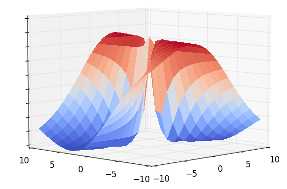
(a) Optimization surface

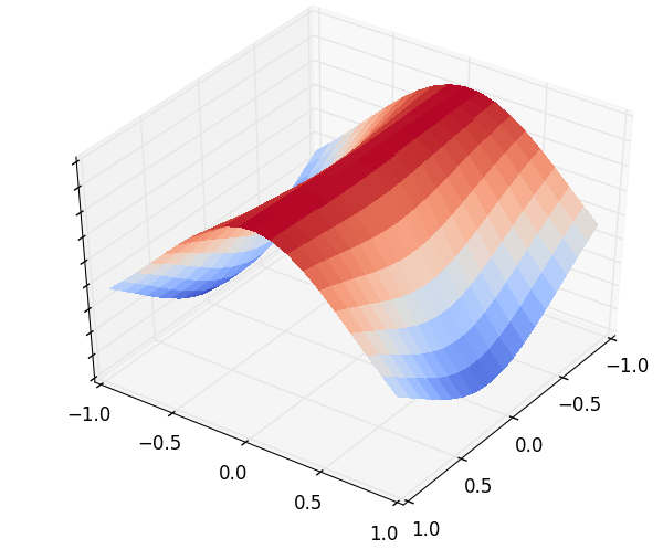
(b) Saddlepoint

Figure 4: Optimization surface for $\text{loss}(\mathbf{D})=\min_{\mathbf{H}}\sum_{t=1}^{T}\|\mathbf{X}_{:t}-\mathbf{D}\mathbf{H}_{:t}\|_{2}^{2}+\alpha\|\mathbf{H}\|_{F}^{2}+\alpha\|\mathbf{D}\|_{F}^{2}$ where $\mathbf{D}\in\mathbb{R}^{2\times 1}$, $T=20$ and $\alpha=0.5$. The first figure illustrates the symmetry of the problem, where there are two equivalent optimal $\mathbf{D}$ in terms of the objective. The second figure is zoomed into the top of the optimization surface, indicating the saddle-point between these two optimal points.

6 Empirical evidence for optimality of alternating minimization for induced DLMs

We now empirically investigate the central hypothesis to this work, to complement the theoretical insights in the previous two sections. We show that for several induced DLMs—including those not directly covered by the theoretical results—that alternating minimization seems to find global solutions. Further, we show that a couple of deviations oustide of this class do not appear to maintain this property. This suggests that the class of induced DLMs identifies a subclass of DLMs that have well-behaved optimization surfaces. We first provide these empirical results and then conclude the section with details about the alternating minimization variants and implementation.

6.1 Optimality of alternating minimization for a variety of DLMs

To test for global optimality, the alternating minimization is started from different initial values and differences in the solution reported. We report both differences in the objective value (Table 2) and in the matrices themselves (Table 3). The normed differences between the solutions $\mathbf{Z}=\mathbf{D}\mathbf{H}$ are reported to clarify that similarities in objectives are due to similar solutions, rather than because the objective itself does not change much. The initializations are random but of highly differing magnitudes to better search for different local minima and saddlepoints in which the optimization could get stuck. Small relative differences between objective values suggest that the stationary points are in fact the same global minimum.

As baselines and to further elucidate if this global optimality property is characteristic of induced DLMs, we also test two modifications that take the objective outside the class of induced DLMs. The first modification is to use $\sum_{i=1}^{d}\|\mathbf{D}_{i:}\|_{2}$ as the regularizer on $\mathbf{D}$, which couples the columns of $\mathbf{D}$ and so is not a valid regularizer for induced DLMs. The second modification is to use the non-norm elastic net regularizer $f_{c}^{2}(\mathbf{d})=\nu\|\mathbf{d}\|_{2}^{2}+(1-\nu)\|\bm{\Lambda}\mathbf{d}\|_{1}$ (Zou and Hastie, 2005), which does not satisfy the requirements of Proposition 1 for generalized induced DLMs. The non-norm elastic net almost satisfies the requirements of Proposition 1, because $f_{c}(\mathbf{d})=\sqrt{\nu\|\mathbf{d}\|_{2}^{2}+(1-\nu)\|\bm{\Lambda}\mathbf{d}\|_{1}}$ is centered and non-negative; however, it is non-convex. For $\bm{\Lambda}=\mathbf{I}$, however, $f_{c}(\mathbf{d})$ is almost a convex function, with only a slight concave bow. We find, in fact, that with $\bm{\Lambda}=\mathbf{I}$, alternating minimization does seem to provide global solutions. However, with different choices of $\bm{\Lambda}$, the $f_{c}$ becomes more non-convex and alternating minimization is no longer global. In the following experiments, we choose $\bm{\Lambda}=\mathop{\mathrm{diag}}(1,2,\ldots,d)$.

The results for the differences in objective values and in solution matrices are summarized in Table 2 and Table 3 respectively. The induced DLMs are in columns 1, 2 and 3 and the modified settings, which no longer correspond to induced DLMs, are in columns 4, 5 and 6. The results are reported across many settings, including $d\in\{5,10,50\}$, $k\in\{3,5,10\}$ and $\alpha\in\{0.005,0.05,0.5\}$, with a fixed sample size of $T=100$ and least-squares $\ell_{2}$ loss. The initial entries in the factors were randomly selected from unit-variance Gaussian distributions with increasing mean values $\mu\in\{0,5,10,15,\ldots,45\}$. For objective values the induced DLMs have relative differences within 0.1%, suggesting they are equivalent global optima, whereas the modified objectives have significantly larger relative differences, between 10% to 150%, demonstrating clearly different local minima. The relative differences between two solutions $\mathbf{Z}_{1}=\mathbf{D}_{1}\mathbf{H}_{1}$ and $\mathbf{Z}_{2}=\mathbf{D}_{2}\mathbf{H}_{2}$ are similarly small, though unsurprisingly larger than the objective values. Particularly for the elastic net, the larger the variable, the more opportunity to select which entries in $\mathbf{Z}$ will be zeroed with similar objective values. The trend, however, remains consistent, with smaller relative differences for the induced DLMs.

	Subspace	Sparse	Elastic Net	Elastic net	Coupled cols	Coupled cols
	$f_{c}^{2}=\|\cdot\|_{2}^{2}$	$f_{c}^{2}=\|\cdot\|_{1}^{2}$	$\nu\|\cdot\|_{2}^{2}+(1-\nu)\|\cdot\|_{1}^{2}$	(non-norm)	$\sum_{i=1}^{d}\|\mathbf{D}_{i:}\|_{1}^{2}$	$\sum_{i=1}^{d}\|\mathbf{D}_{i:}\|_{2}$
	$f_{r}^{2}=\|\cdot\|_{2}^{2}$	$f_{r}^{2}=\|\cdot\|^{2}_{1}$	$\nu_{\textrm{D}}=0.5=\nu_{\textrm{H}}$	$\nu_{\textrm{D}}=0.5=\nu_{\textrm{H}}$	$f_{r}^{2}=\|\cdot\|_{2}^{2}$	$f_{r}^{2}=\|\cdot\|_{2}^{2}$
30cm Min Difference	30cm30cm 0.000000 $(0.5,5,10)$	30cm 0.000000 $(0.05,5,3)$	30cm 0.000000 $(0.5,5,3)$	30cm 0.000007 $(0.05,50,3)$	30cm 0.004586 $(0.5,10,3)$	30cm 0.466634 $(0.005,5,3)$
30cm Max Difference	30cm 0.000785 $(0.005,5,5)$	30cm 0.000136 $(0.5,50,10)$	30cm 0.001269 $(0.05,10,10)$	30cm 1.535013 $(0.005,50,3)$	30cm 0.096123 $(0.005,5,3)$	30cm 0.566597 $(0.05,10,3)$

Table 2: The minimum and maximum relative differences between objective values for the solutions found by alternating minimization, with a least-squares loss and the given regularizers. The relative difference between a pair of solutions is computed by taking the absolute difference between their objective values divided by the expected value of the objective across the solutions (to normalize the magnitude for changing $d,k$). The parameter settings that resulted in the minimum and maximum relative difference are reported in brackets below the values with the order $(\alpha,d,k)$.

	Subspace	Sparse	Elastic Net	Elastic net	Coupled cols	Coupled cols
	$f_{c}^{2}=\|\cdot\|_{2}^{2}$	$f_{c}^{2}=\|\cdot\|_{1}^{2}$	$\nu\|\cdot\|_{2}^{2}+(1-\nu)\|\cdot\|_{1}^{2}$	(non-norm)	$\sum_{i=1}^{d}\|\mathbf{D}_{i:}\|_{1}^{2}$	$\sum_{i=1}^{d}\|\mathbf{D}_{i:}\|_{2}$
	$f_{r}^{2}=\|\cdot\|_{2}^{2}$	$f_{r}^{2}=\|\cdot\|^{2}_{1}$	$\nu_{\textrm{D}}=0.5=\nu_{\textrm{H}}$	$\nu_{\textrm{D}}=0.5=\nu_{\textrm{H}}$	$f_{r}^{2}=\|\cdot\|_{2}^{2}$	$f_{r}^{2}=\|\cdot\|_{2}^{2}$
30cm Min Difference	30cm30cm 0.000000 $(0.005,5,3)$	30cm 0.000000 $(0.05,5,3)$	30cm 0.000000 $(0.5,5,3)$	30cm 0.000000 $(0.5,5,3)$	30cm 0.007800 $(0.005,50,3)$	30cm 0.004000 $(0.05,5,10)$
30cm Max Difference	30cm 0.005000 $(0.05,10,10)$	30cm 0.023400 $(0.05,50,3)$	30cm 0.124800 $(0.5,50,10)$	30cm 0.994400 $(0.5,50,3)$	30cm 0.631000 $(0.5,10,10)$	30cm 0.592000 $(0.005,50,3)$

Table 3: The minimum and maximum relative norm differences between solutions found by alternating minimization, with a least-squares loss and the given regularizers. The relative difference is a thresholded relative difference, illustrating the percentage of significantly different values. The relative difference between two solutions is the number of entries above the threshold 0.05, in terms of the absolute value of the difference between the two solutions $\mathbf{Z}_{1}=\mathbf{D}_{1}\mathbf{H}_{1}$ and $\mathbf{Z}_{2}=\mathbf{D}_{2}\mathbf{H}_{2}$, divided by the total number of elements. The parameter settings that resulted in the minimum and maximum are reported in brackets below the values with the order $(\alpha,d,k)$.

6.2 Selecting the inner dimension

The optimality of induced DLMs has been predicated on selecting a sufficiently large inner dimension $k$. Because $k$ can be critical, it is important to understand how to set this parameter. For certain models, the selection of $k$ is intuitive. For example, for subspace dictionary learning, $k$ is the size of the desired latent rank, where $k$ can be chosen smaller for larger values of $\alpha$. For sparse coding, the increase in the $\alpha$ does not naturally lead to a decrease in $k$, but rather to an increase in the level of sparsity. For the elastic net regularizer, however, we have less intuition; there is likely a preference for $d<k<T$, but this remains unknown.

There are several strategies that can be pursued to facilitate choice of $k$. A simple approach is to allow the optimization to select $k$ by setting $k=T$. The optimal solution will have an implicit $k$ that is smaller than $T$. This approach, however, is typically not computationally feasible. To avoid setting $k$ too large, a number of algorithms have been developed that iteratively generate columns and rows to add to $\mathbf{D}$ and $\mathbf{H}$ respectively d’Aspremont et al. (2004); Bach et al. (2008); Journée et al. (2010); Zhang et al. (2012); Hsieh and Olsen (2014); Mirzazadeh et al. (2015). In practice, however, it is common to simply choose a fixed $k$; such a strategy, however, compromises some of the simplicity and efficiency of a standard alternating minimization algorithm, initialized from a random solution. Despite the introduction of such algorithms, it remains common in practice to simply choose a fixed $k$ and using alternating minimization. Further, it is less clear how to extend such algorithms, that iteratively increase $k$, to the incremental setting.

To facilitate the use of the simple alternating minimization approach used in practice, for a fixed user-specified $k$, we show the optimality properties of subspace, sparse and elastic-net DLMs, for increasing $k$. The goal of these exploratory results is to better elucidate practical choices of $k$ for these induced DLMs. The results are reported on the Extended Yale Face Database B Georghiades et al. (2001). We provide two experiments. The first parallels the experiments in the previous section, but now we test optimality for a variety of $k$, including small $k$. The second experiment is to determine how much the objective can be improved by increasing $k$. The goal of the first experiment is to examine for which user-specified $k$, alternating minimization can find global solutions. The goal of the second experiment is to examine the inherent preference in the objective for a larger $k$.

For the first comparison, we determine the optimality of alternating minimization for smaller $k$, shown in Figure 5. This contrasts the results in the previous section, where we fixed $k$ to one, larger value. The theoretical results indicate that even if $k$ is less than the dimension $k^{*}$ that gives $\mathrm{R}_{k}={\mathrm{R}_{\mathrm{\scriptsize Z}}}$, alternating minimization can still give global solutions for $k$ that results in convex $\mathrm{R}_{k}$. We find that for even very small $k$, alternating minimization produces global solutions. This is a surprising result, considering for sparse coding ($\nu_{\textrm{H}}=0$), the conventional wisdom is that $k$ needs to be quite large (close to $T$) to get optimal solutions. Here, however, we are showing that alternating minimization, with a restricted $k$, can still obtain the global solution for that objective. When comparing to an objective where $k$ is allowed to be larger, there is a bigger difference (see Figure 6). Therefore, if a specific $k$ is desired for sparse coding, alternating minimization is likely going to reach the global minimum, despite the fact that further increasing $k$ could further decrease the objective. This behavior suggests that either $\mathrm{R}_{k}$ is convex for these $k$, or potentially that $\mathrm{R}_{k}$ has other nice properties not currently characterized by our theory. We discuss this outcome further in the conclusion.

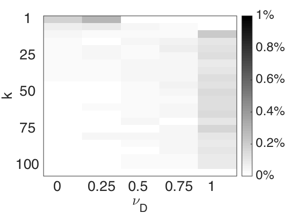
(a) $\nu_{\textrm{H}}$ = 0

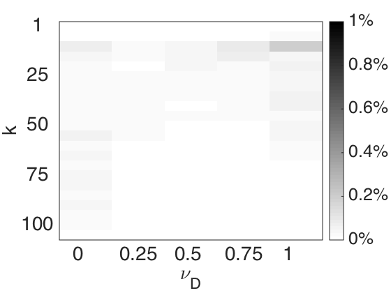
(b) $\nu_{\textrm{H}}$ = 0.5

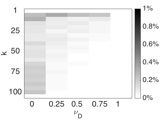
(c) $\nu_{\textrm{H}}$ = 1.0

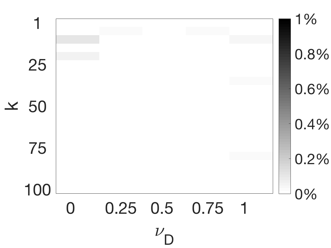
(d) $\nu_{\textrm{H}}$ = 0

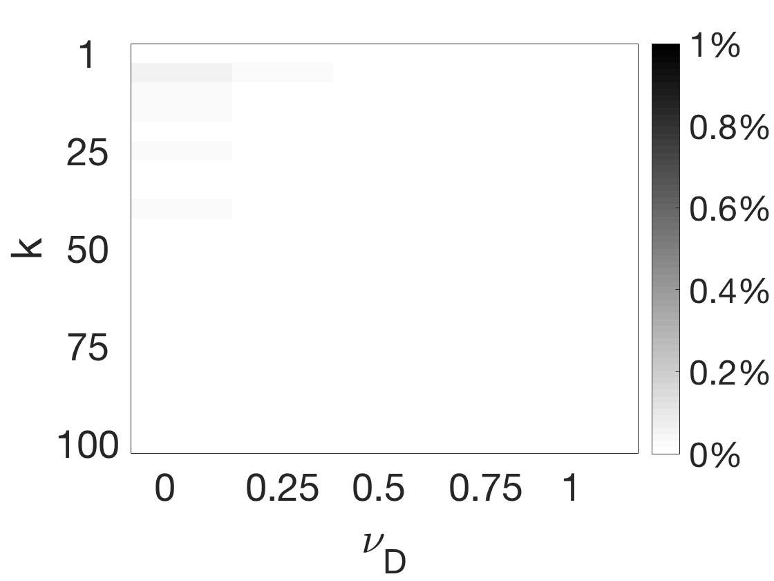
(e) $\nu_{\textrm{H}}$ = 0.5

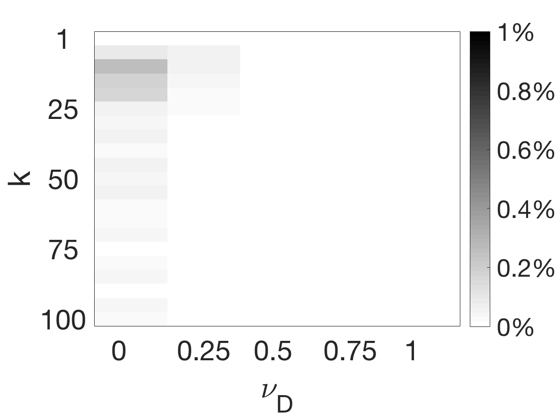
(f) $\nu_{\textrm{H}}$ = 1.0

Figure 5: Standard deviations of the objective value for $k\leq T$ for elastic net DLMs, over 10 runs of different random initializations with the same regularization parameters. The lighter the color, the smaller the difference. The loss is the least-squares loss for (a) - (c), and the logistic loss for (d) - (f), with $T=100$ and $d=50$ on data randomly drawn from the Extended Yale Face Database B. The relative differences are averaged over 10 runs, with the maximal distance reported within each run from 10 different random initializations. The goal is to identify if the solutions returned for highly different initial points result in different local minima. The standard deviation is very small for all choices of $k$, suggesting that the AM-DLM  algorithm (see Algorithm 1) obtains a globally optimum solution even for small $k$.

For the second experiment, we compare the objective values for increasing sizes of $k$, compared to the least constrained setting of $k=T$. The results are summarized in Figure 6. We expect that if the objective has a strong preference for larger $k$, then there will be a large discrepancy between the objective value for small $k$ and the objective value for $k=T$. The result indicates that $k$ can be much smaller than $T$ and obtain good solutions, within $1\%$. Recall that $\nu_{\textrm{D}}=0$ results in a sparse $\ell_{1}$ regularizer on $\mathbf{D}$, and $\nu_{\textrm{D}}=1$ results in the subspace $\ell_{2}$ regularizer on $\mathbf{D}$. The cases where $k$ needs to be larger to match performance of $k=T$ are when $\nu_{\textrm{D}}=0,\nu_{\textrm{H}}=1$ or $\nu_{\textrm{D}}=1,\nu_{\textrm{H}}=0$. This is consistent with previous results, where the global solution for sparse coding requires $k=T$. We can see that even with a small decrease from this extreme setting, with $\nu_{\textrm{D}}<1,\nu_{\textrm{H}}=0$, $k$ can be significantly smaller without incurring much difference to the optimal solution at $k=T$. Therefore, for sparse coding ($\nu_{\textrm{H}}=0$ and $\nu_{\textrm{D}}=1$), the choice of $k$ does need to be noticeably larger than for the elastic net (i.e., all other settings). This validates the initial motivation for using the elastic-net for dictionary learning, for learning more compact sparse representations.

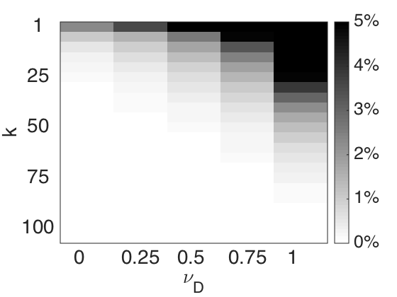
(a) $\nu_{\textrm{H}}$ = 0

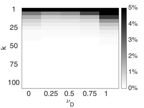
(b) $\nu_{\textrm{H}}$ = 0.5

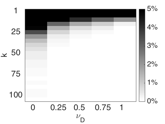
(c) $\nu_{\textrm{H}}$ = 1.0

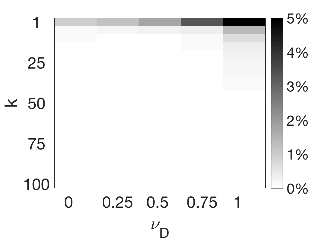
(d) $\nu_{\textrm{H}}$ = 0

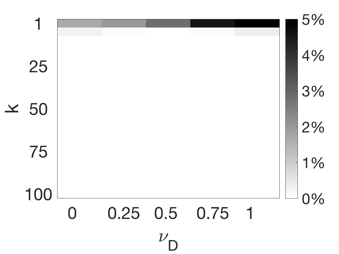
(e) $\nu_{\textrm{H}}$ = 0.5

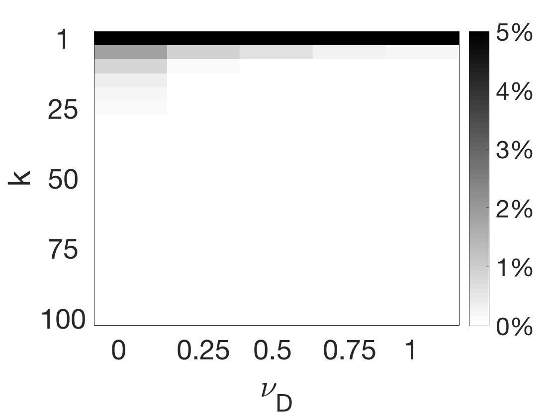
(f) $\nu_{\textrm{H}}$ = 1.0

Figure 6: Comparison between the objective value for $k<T$ and $k=T$ for the elastic net DLMs. The reported relative differences are computed between the objective value for $k$ and the objective values at $k=T$, normalized by the objective value at $k=T$ to give a percentage difference. The lighter the color, the smaller the difference. The loss is the least-squares loss for (a) - (c), and the logistic loss for (d) - (f), with $T=100$ and $d=50$ on data randomly drawn from the Extended Yale Face Database B. The relative differences are averaged over 10 runs, with the maximal distance reported within each run from 10 different random initializations.

6.3 Batch optimization algorithm for induced DLMs

In this section, we include algorithmic details on the alternating minimization. We opt for a basic alternating minimization strategy, without specific initialization or explicit strategies to escape saddle points. In particular, we focus only on making the alternating minimization more effective by improving the convergence rate in two ways: (a) using an incomplete alternating minimization and (b) deriving a proximal operator for the squared $\ell_{2}$ norm, required for both the sparse coding and elastic net DLMs.

The alternating minimization algorithm for DLMs—summarized in Algorithm 1— is a standard block coordinate descent algorithm, with a few specific choices that we found effective. The standard approach involves descending in one variable with the other fixed, and then alternating. The main algorithmic choices are to use inexact updates for the alternating minimization, with proximal gradient updates for non-smooth regularizers. Empirically, we found both these modifications significantly speed convergence. We opt for proximal gradient approaches rather than other approaches, such as the alternating direction method of multipliers, because it maintains sparse variables which can be more efficiently stored and because the convergence results for proximal gradient approaches are well understood, even under approximate updates Machart et al. (2012).

Inexact alternating step.

To alternate between $\mathbf{D}$ and $\mathbf{H}$ in the optimization, one can completely solve for each variable with the other fixed (exact) or alternate between single gradient descent steps (inexact). Both approaches converge under general conditions, proven as part of more general results about the convergence of block coordinate descent for multi-convex problems using exact updates Xu and Yin (2013) and inexact updates Tappenden et al. (2014). In our own experiments, we found the exact updates significantly slower and only marginally less sensitive to parameter choices, such as the step-size. We therefore adopt the inexact method, which is significantly faster.

Algorithm 1 Alternating Minimization for Dictionary Learning Models (AM-DLM)

$\triangleright$ Input loss components $\mathrm{L}$, ${\mathrm{R}_{\mathrm{\scriptsize D}}}$, ${\mathrm{R}_{\mathrm{\scriptsize H}}}$, $k$

$\mathbf{D},\mathbf{H}\leftarrow$ random full-rank matrices with inner dimension $k$

prevobj $\leftarrow\infty$

repeat

     Update $\mathbf{D}$ using one step of gradient descent (such as in Algorithms 2, 3 or 4)

     Update $\mathbf{H}$ using one step of gradient descent (such as in Algorithms 2, 3 or 4)

     currentobj $\leftarrow\mathrm{L}(\mathbf{D}\mathbf{H})+{\mathrm{R}_{\mathrm{\scriptsize D}}}(\mathbf{D})+{\mathrm{R}_{\mathrm{\scriptsize H}}}(\mathbf{H})$

     if $|\text{currentobj}-\text{prevobj}|<$ tolerance then break      

     prevobj $\leftarrow$ currentobj

until convergence within tolerance or reach maximum number of iterations

return $\mathbf{D},\mathbf{H}$

Algorithm 2 Standard gradient descent step for smooth regularizers

$\mathbf{D}\leftarrow\mathbf{D}-\eta_{D}(\nabla_{Z}\mathrm{L}(\mathbf{D}\mathbf{H})\mathbf{H}^{\top}+\nabla_{D}{\mathrm{R}_{\mathrm{\scriptsize D}}}(\mathbf{D}))$ $\triangleright$ $\mathbf{H}$ update: $\mathbf{H}\leftarrow\mathbf{H}-\eta_{H}(\mathbf{D}^{\top}\nabla_{Z}\mathrm{L}(\mathbf{D}\mathbf{H})+\nabla_{H}{\mathrm{R}_{\mathrm{\scriptsize H}}}(\mathbf{H}))$

Algorithm 3 Proximal gradient descent step for $\ell_{1}$ regularizer

$\triangleright$ The steps are written for updating $\mathbf{D}$ with fixed $\mathbf{H}$. Differences in the updates to $\mathbf{H}$ are in comments.

$\Delta\leftarrow\nabla\mathrm{L}(\mathbf{D}\mathbf{H})\mathbf{H}^{\top}$ $\triangleright$ $\mathbf{H}$ update: $\Delta\leftarrow\mathbf{D}^{\top}\nabla\mathrm{L}(\mathbf{D}\mathbf{H})$

$l\leftarrow$ the Lipschitz constant of the gradient (or an upper bound to the constant)

for all $j$ do

     for all $i$ do $\triangleright$ $\mathbf{H}$ update: swap indices to update one row at a time

         $\mathbf{D}_{ij}=\mathrm{sign}(\mathbf{D}_{ij}-\Delta_{ij}/l)\max(|\mathbf{D}_{ij}-\Delta_{ij}/l|-\frac{\alpha}{l},0)$      

     $\Delta\leftarrow\nabla\mathrm{L}(\mathbf{D}\mathbf{H})\mathbf{H}^{\top}$ $\triangleright$ $\mathbf{H}$ update: $\Delta\leftarrow\mathbf{D}^{\top}\nabla\mathrm{L}(\mathbf{D}\mathbf{H})$

Algorithm 4 Proximal gradient descent step for elastic net regularizer with $\ell_{1}^{2}$

repeat

     for $i=1$ to $k$ do

         $\triangleright$ Calculate Lipschitz constant. For example, if $\mathrm{L}$ is the least-squares loss, then

         $\triangleright$ for the $\mathbf{D}$ update: $l\leftarrow 2(\|\mathbf{H}_{i:}\|_{1}^{2}+\nu_{\textrm{D}}\alpha)$ or for the $\mathbf{H}$ update: $l\leftarrow 2(\|\mathbf{D}_{:i}\|_{1}^{2}+\nu_{\textrm{H}}\alpha/s)$

         $l\leftarrow$ the Lipschitz constant of the gradient (or an upper bound to the constant)

         Update $\mathbf{D}_{:i}$ (or $\mathbf{H}_{i:}$) using Algorithm 5 with current $\mathbf{D}$ (or $\mathbf{H}$)      

until difference between $\mathbf{D}$ (or $\mathbf{H}$) on successive steps within tolerance or maximum number of iterations

Algorithm 5 Soft thresholding algorithm for updating column vectors of $\mathbf{D}$

$\lambda\leftarrow\tfrac{(1-\nu_{\textrm{D}})\alpha}{l}$ $\triangleright$ To update $\mathbf{H}$: $\lambda\leftarrow\tfrac{(1-\nu_{\textrm{H}})\alpha}{sl}$

repeat

     $\mathbf{u}\leftarrow\mathbf{D}_{:i}-\tfrac{1}{l}[\nabla\mathrm{L}(\mathbf{D}\mathbf{H})\mathbf{H}_{i:}^{\top}+2\nu_{\textrm{D}}\alpha\mathbf{D}_{:i}]$ $\triangleright$ $\mathbf{H}$ update: $\mathbf{u}\leftarrow\mathbf{H}_{i:}-\tfrac{1}{l}[\mathbf{D}_{:i}^{\top}\nabla\mathrm{L}(\mathbf{D}\mathbf{H})+2\nu_{\textrm{H}}\alpha/s\mathbf{H}_{i:}]$

     Sort $\mathbf{u}=[u_{1},\ldots,u_{k}]$ according to $\left|u_{i}\right|$ in descending order such that $\left|u_{m_{1}}\right|\geq\left|u_{m_{2}}\right|\geq...\geq\left|u_{m_{k}}\right|$

     $C\leftarrow 0,r\leftarrow 0$,

     while $r<k$ and $\left|u_{m_{r+1}}\right|>\tfrac{2\lambda C}{1+2\lambda r}$ do

         $C\leftarrow C+\left|u_{m_{r+1}}\right|$

         $r\leftarrow r+1$      

     for $j=1$ to $k$ do

         $\mathbf{D}_{ij}\leftarrow\mathrm{sign}(u_{j})\max\left(\left|u_{j}\right|-\tfrac{2\lambda C}{1+2\lambda r},0\right)$ $\triangleright$ $\mathbf{H}$ update: flip indices to update $\mathbf{H}_{ji}$      

until difference between $\mathbf{D}$ on successive steps within tolerance or reach maximum number of iterations

Proximal gradient updates.

A standard gradient descent step is problematic when the regularizer, or a component of the regularizer, is non-differentiable. For example, $\ell_{1}$ has a non-differentiable point at $0$. Though one could simply choose a subgradient at $0$ and apply subgradient descent, in practice for batch optimization, the convergence properties are poor. For alternating minimization on induced DLMs, we found that the descent would converge to a point and then very slowly decrease over a large number of iterations.

Proximal gradient methods, on the other hand, use a proximal operator that avoids computation of the subgradient of the non-differentiable component. For example, for the $\ell_{1}$ regularizer, with Lipschitz constant $l$ for the gradient of the loss, the proximal operator is the soft-thresholding operator

$$\text{prox}(\mathbf{u})=\mathop{\mathrm{argmin}}_{\mathbf{u}\in\mathbb{R}^{T}}\frac{1}{2}\|\mathbf{u}-\mathbf{h}\|_{2}^{2}+\frac{\alpha}{l}\|\mathbf{h}\|_{1}=\mathrm{sign}(\mathbf{u})\circ\max(|\mathbf{u}|-\frac{\alpha}{l},\mathbf{\bm{0}})$$

where the multiplication $\circ$ is element-wise. Proximal operators are well-known for common non-smooth regularizers such as $\|\cdot\|_{1}$ and $\|\cdot\|_{2}$ Bach et al. (2011). Some regularizers for induced DLMs, however, involve squares of convex functions, which is atypical. For example, $\|\cdot\|_{1}^{2}$ is used in the elastic net DLM. To the best of our knowledge, proximal operators have not been derived for $\|\cdot\|_{1}^{2}$. We provide the proximal updates for the elastic net DLM  in Algorithm 4 and 5, with proof of the validity of the operator in Proposition 18 in Appendix F.

7 Incremental estimation

In this section, we explore how to effectively learn $\mathbf{D}$ incrementally. We discuss an incremental algorithm for least-squares losses that summarizes past data (online AM-DLM) and discuss how to use stochastic gradient descent updates. We provide experiments demonstrating the different properties of the online versus stochastic incremental algorithms, particularly providing insights into step-size selection.

7.1 Online AM-DLM  algorithm

For a least-squares loss, a more sample efficient incremental algorithm can be used to optimize induced DLMs. This algorithm is summarized in Algorithm 6. It is a straightforward modification of Mairal et al. (2010, Algorithm 1), which was introduced for sparse coding and for which they proved convergence to stationary points (Mairal et al., 2010, Proposition 1). The main modification is to use a regularizer on $\mathbf{D}$ instead of a projection onto a constraint set. Note that Mairal et al. (2010, Section 3.4) discuss several algorithmic improvements, including down-weighting past samples and using mini-batches; these ideas extend directly to this algorithm and so we do not repeat them here.

Algorithm 6 Online AM-DLM

$\triangleright$ Input full rank initial dictionary $\mathbf{D}_{0}\in\mathbb{R}^{d\times k}$, $T$ as number of iterations

$\mathbf{A}_{0}\leftarrow\mathbf{\bm{0}}\in\mathbb{R}^{k\times k}$, $\mathbf{B}_{0}\leftarrow\mathbf{\bm{0}}\in\mathbb{R}^{d\times k}$

for $t=1$ to $T$ do

     $\triangleright$ If multiple passes over a dataset, reshuffle the data for each pass

     $\triangleright$ As before, if there is a non-smooth regularizer on $\mathbf{D}$ or $\mathbf{H}$, then use proximal updates

     $\mathbf{h}_{t}\leftarrow\mathop{\mathrm{argmin}}_{\mathbf{h}\in\mathbb{R}^{k}}\frac{1}{2}\left\|\mathbf{D}_{t-1}\mathbf{h}-\mathbf{x}_{t}\right\|_{2}^{2}+{\mathrm{R}_{\mathrm{\scriptsize H}}}(\mathbf{h})$

     $\beta_{t}\leftarrow\max(\tfrac{1}{t},0.01)$

     $\mathbf{A}_{t}\leftarrow(1-\beta_{t})\mathbf{A}_{t-1}+\beta_{t}\mathbf{h}_{t}\mathbf{h}_{t}^{\top}$

     $\mathbf{B}_{t}\leftarrow(1-\beta_{t})\mathbf{B}_{t-1}+\beta_{t}\mathbf{x}_{t}\mathbf{h}_{t}^{\top}$

     Compute $\mathbf{D}_{t}$ using $\mathbf{D}_{t-1}$ as initial point (warm restart)

$$\mathbf{D}_{t} =\mathop{\mathrm{argmin}}_{\mathbf{D}\in\mathbb{R}^{d\times k}}\frac{1}{t}\sum_{i=1}^{t}\left(\frac{1}{2}\left\|\mathbf{D}\mathbf{h}_{i}-\mathbf{x}_{i}\right\|_{2}^{2}+{\mathrm{R}_{\mathrm{\scriptsize H}}}(\mathbf{h}_{i})\right)+{\mathrm{R}_{\mathrm{\scriptsize D}}}(\mathbf{D})$$

$$=\mathop{\mathrm{argmin}}_{\mathbf{D}\in\mathbb{R}^{d\times k}}\frac{1}{2}\mathop{\mathrm{tr}}\left(\mathbf{D}^{\top}\mathbf{D}\mathbf{A}_{t}\right)-\mathop{\mathrm{tr}}\left(\mathbf{D}^{\top}\mathbf{B}_{t}\right)+{\mathrm{R}_{\mathrm{\scriptsize D}}}(\mathbf{D})$$

return $\mathbf{D}_{T}$

$\triangleright$ If it takes at most $S$ descent iterations to get $\mathbf{h}_{t}$ or $\mathbf{D}_{t}$, then the time complexity for each $t$ is $O(Sdk^{2})$

Algorithm 7 SGD AM-DLM

$\triangleright$ Input full rank initial dictionary $\mathbf{D}_{0}\in\mathbb{R}^{d\times k}$, $T$ as number of iterations

for $t=1$ to $T$ do

     $\triangleright$ If multiple passes over a dataset, reshuffle the data for each pass

     $\triangleright$ If there is a non-smooth regularizer on $\mathbf{H}$, use sub-gradient descent to get $\mathbf{h}$

     $\mathbf{h}_{t}\leftarrow\mathop{\mathrm{argmin}}_{\mathbf{h}\in\mathbb{R}^{k}}L_{x}(\mathbf{D}_{t-1}\mathbf{h},\mathbf{x}_{t})+{\mathrm{R}_{\mathrm{\scriptsize H}}}(\mathbf{h})$

     $\triangleright$ Update $\mathbf{D}_{t}$ using one step of stochastic subgradient descent step

     Select step-size $\eta_{t}$ as described in Section 7.2

     $\mathbf{D}_{t}\leftarrow\mathbf{D}_{t-1}-\eta_{t}(\nabla l_{t}(\mathbf{D}_{t-1})+\nabla{\mathrm{R}_{\mathrm{\scriptsize D}}}(\mathbf{D}_{t-1}))$ $\triangleright$ $\nabla l_{t}(\mathbf{D}_{t-1})=\nabla L_{x}(\mathbf{D}_{t-1}\mathbf{h},\mathbf{x}_{t})\mathbf{h}^{\top}$

return $\mathbf{D}_{T}$

$\triangleright$ If it takes at most $S$ descent iterations to get $\mathbf{h}_{t}$ or $\mathbf{D}_{t}$, then the time complexity for each $t$ is $O(Sdk)$. The time complexity for the step-size selection strategies, is dominated by this; for accelerated SG, the time complexity is $O(d+k)$, and for the others is constant.

7.2 Stochastic gradient descent for DLMs

Stochastic gradient descent (SGD) is another approach to incremental estimation of DLMs. As discussed in Section 3.4, only $\mathbf{D}$ is updated incrementally, according to the loss

$$l_{t}(\mathbf{D})={\mathrm{R}_{\mathrm{\scriptsize D}}}(\mathbf{D})+\big{(}\min_{\mathbf{h}}L_{x}(\mathbf{D}\mathbf{h},\mathbf{x}_{t})+{\mathrm{R}_{\mathrm{\scriptsize H}}}(\mathbf{h})\big{)}.$$ (25)

Therefore, on each step, the optimal $\mathbf{h}$ is computed for the current $\mathbf{D}$ and data point $\mathbf{x}_{t}$, and then a gradient step is performed for $\mathbf{D}$ using $l_{t}(\mathbf{D})$. Unlike online AM-DLM, we used subgradient descent updates for both $\mathbf{h}$ and $\mathbf{D}$ for SGD AM-DLM. Using proximal gradient updates for either $\mathbf{h}$ or $\mathbf{D}$ resulted in $\mathbf{h}$ becoming progressively more sparse and the resulting solution was poor. This remains an important open question for future work in using stochastic gradient descent for induced DLMs. We summarize the SGD choices we found to be effective, in Algorithm 7.

We will empirically investigate which of these two incremental algorithms is generally more effective for optimizing induced DLMs incrementally. The SGD algorithm is significantly faster per-step, scaling as $O(dk)$, compared to online AM-DLM, which scales as $O(dk^{2})$. Additionally, the SGD algorithm allows for more general losses, whereas online AM-DLM is restricted to the least-squares loss. However, we expect that online AM-DLM should be more sample efficient. Further, it should be simpler to select step-sizes for online AM-DLM, because line search can be used for the two optimizations within the loop. For SGD, we will need to explore alternative heuristics for setting the step-size.

The key factor for making SGD effective for induced DLMs is to incorporate recent accelerations to SGD. Mairal et al. (2009a) found that for sparse coding, their online AM-DLM  algorithm converged more quickly in terms of samples than SGD. We find, however, that this is not always the case, particularly by taking advantage of the recent understanding of accelerations to stochastic gradient descent (Roux et al. (2012) provide a nice summary). Several of these accelerations rely on strategies for selecting the step-size, $\eta_{t}$. We explored several of these accelerations, and report results for the two that were the most effective with induced DLMs and that did not involve storing gradients.

Accelerated SG.

The first acceleration involves an aggressive step-size selection strategy that enables a constant step-size for several iterations. This strategy gives a more aggressive step-size, that can speed convergence, but that adaptively is decreased to ensure convergence Kesten (1958). On each step, the step-size is only decreased when the inner-product between two successive gradient estimates are negative. Specifically, a list of strictly decreasing step sizes is predefined, with $\eta_{0}$ initialized to the first step size in this list. If $\mathop{\mathrm{tr}}(\nabla l_{t}(\mathbf{D}_{t-1})^{\top}\nabla l_{t}(\mathbf{D}_{t-2}))\geq 0$, then $\eta_{t}=\eta_{t-1}$; otherwise, the step-size is chosen such that $\eta_{t}<\eta_{t-1}$, from the list of step-sizes.

Momentum.

The second acceleration uses a momentum term, which is the difference between two successive iterations (see for example the algorithm by Tseng (1998)). The update for $\mathbf{D}$ is instead

$$\mathbf{D}_{t}\leftarrow\mathbf{D}_{t-1}-\eta_{t}(\nabla l_{t}(\mathbf{D}_{t-1})+\nabla{\mathrm{R}_{\mathrm{\scriptsize D}}}(\mathbf{D}_{t-1}))+\beta_{t}(\mathbf{D}_{t-1}-\mathbf{D}_{t-2})$$

Without the momentum term, $\mathbf{D}_{t-1}-\mathbf{D}_{t-2}=-\eta_{t-1}\nabla l(\mathbf{D}_{t-2})$. The momentum term is stepping further along the direction of this previous gradient. Momentum’s acceleration effects are mainly supported by theories in batch optimization, and has not been theoretically characterized for stochastic settings Sutskever et al. (2013). In practice, however, momentum is typically combined with SGD. Our experiments in Section 7.3 show that adding momentum term can accelerate SGD AM-DLM, but not always.

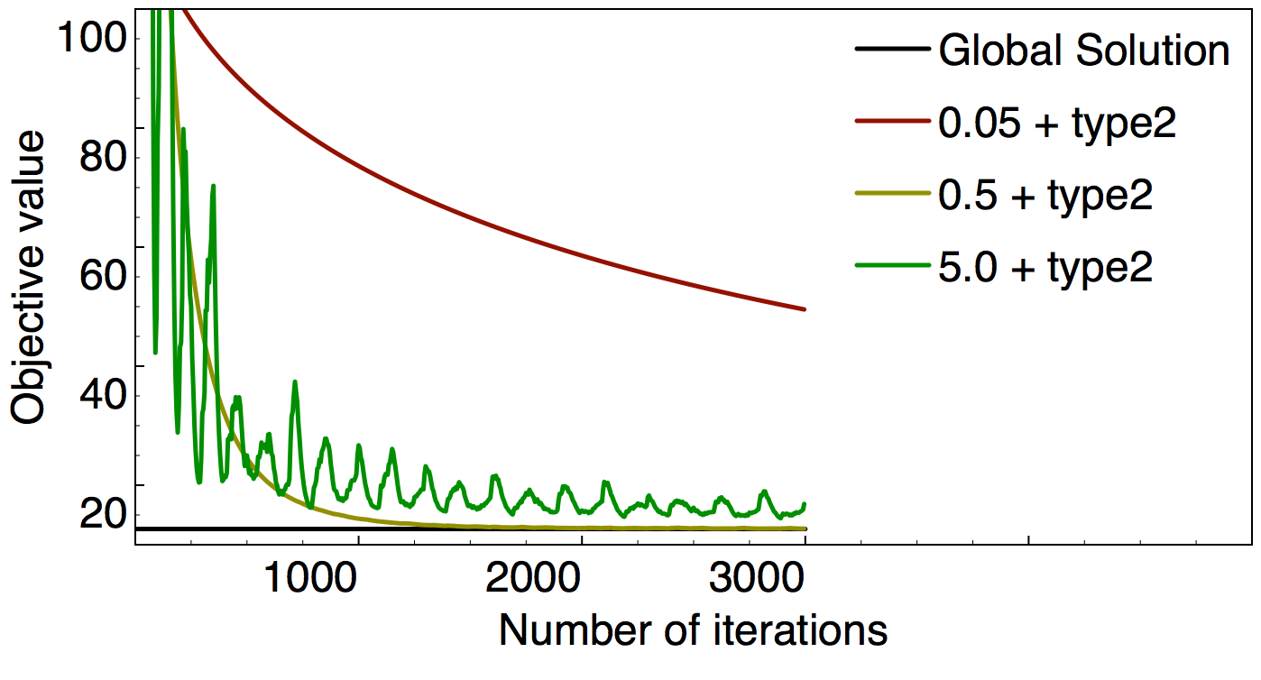
(a) Subspace

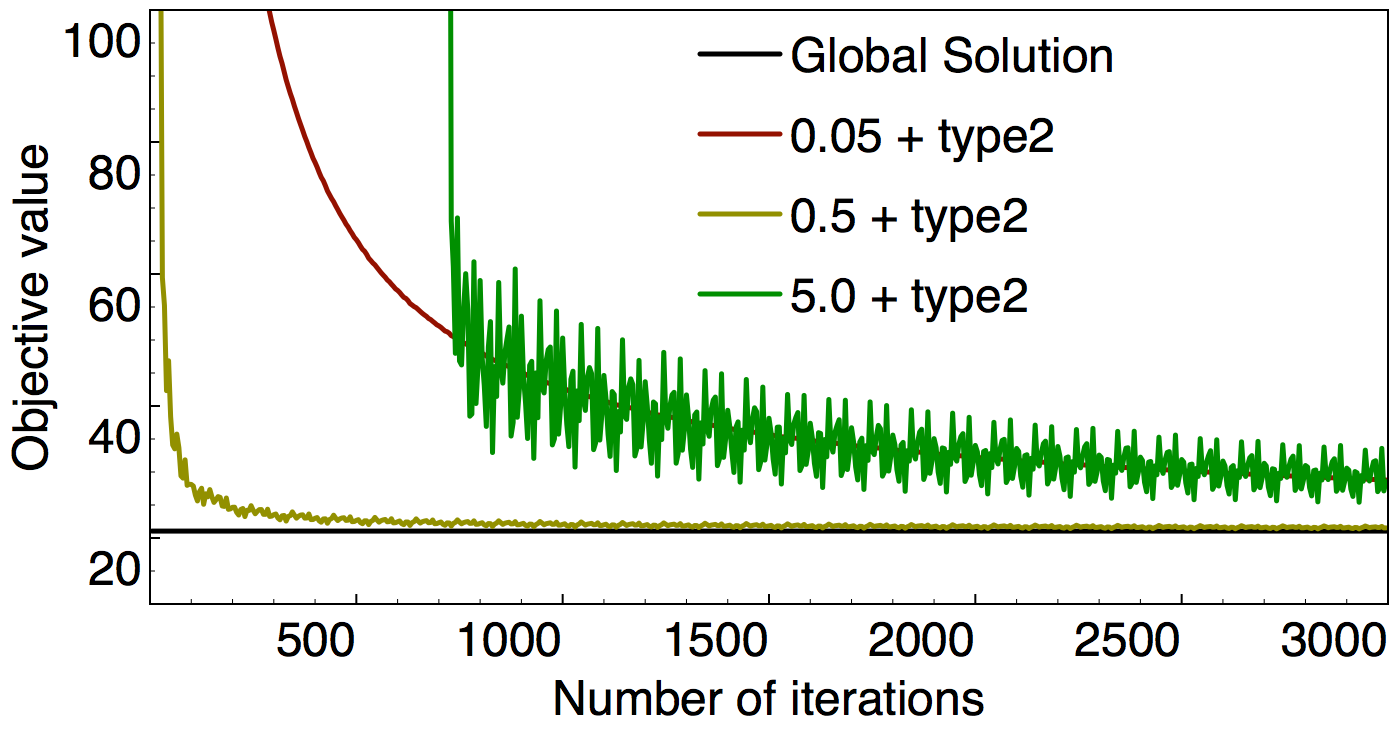
(b) Elastic Net ($\nu_{\textrm{H}}=1.0,\nu_{\textrm{D}}=0.5$)

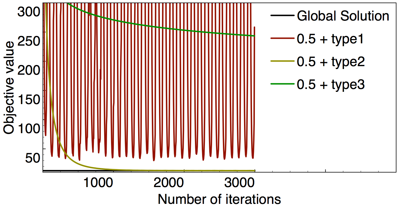
(c) Subspace

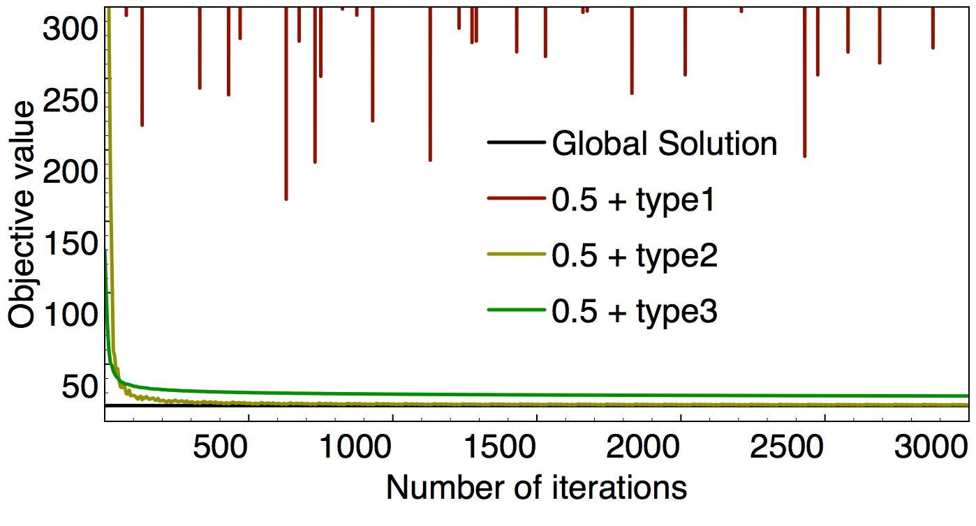
(d) Elastic net ($\nu_{\textrm{H}}=1.0,\nu_{\textrm{D}}=0.5$)

Figure 7: Comparison of SGD AM-DLM  to the global solution for varying $\alpha_{0}$ and step-size decays. The initial step-size is $\eta_{0}\in\{0.05,0.5,5.0\}$. There are three time-based decays to get $\eta_{t}$: $\eta_{0}$ (type 1), $\eta_{0}/\sqrt{t}$ (type 2) and $\eta_{0}/t$ (type 3). In general, we found type 2 to perform the best across $\eta_{0}$, and found $\eta_{0}=0.5$ to produce the fastest, most stable convergence. We therefore more specifically report results for these two settings, with (a), (b) for type 2 with varying $\eta_{0}$ and (c), (d) for $\eta_{0}=0.5$ and varying types. These results indicate that learning can be significantly different across these choices. As expected, an aggressive initial step-size of $5.0$ produces oscillations, though it does in fact converge with the type 2 decay schedule. A conservative step-size of $0.05$ converges too slowly, and an overly fast decay (type 3) may converge before reaching global optima. Setting $\eta_{0}=0.5$ and using type 2 decay converges to a global solution quickly and smoothly.

(a) Subspace

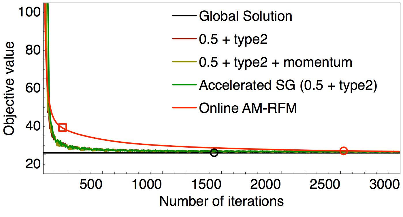
(b) Elastic net ($\nu_{\textrm{H}}=1.0,\nu_{\textrm{D}}=0.5$)

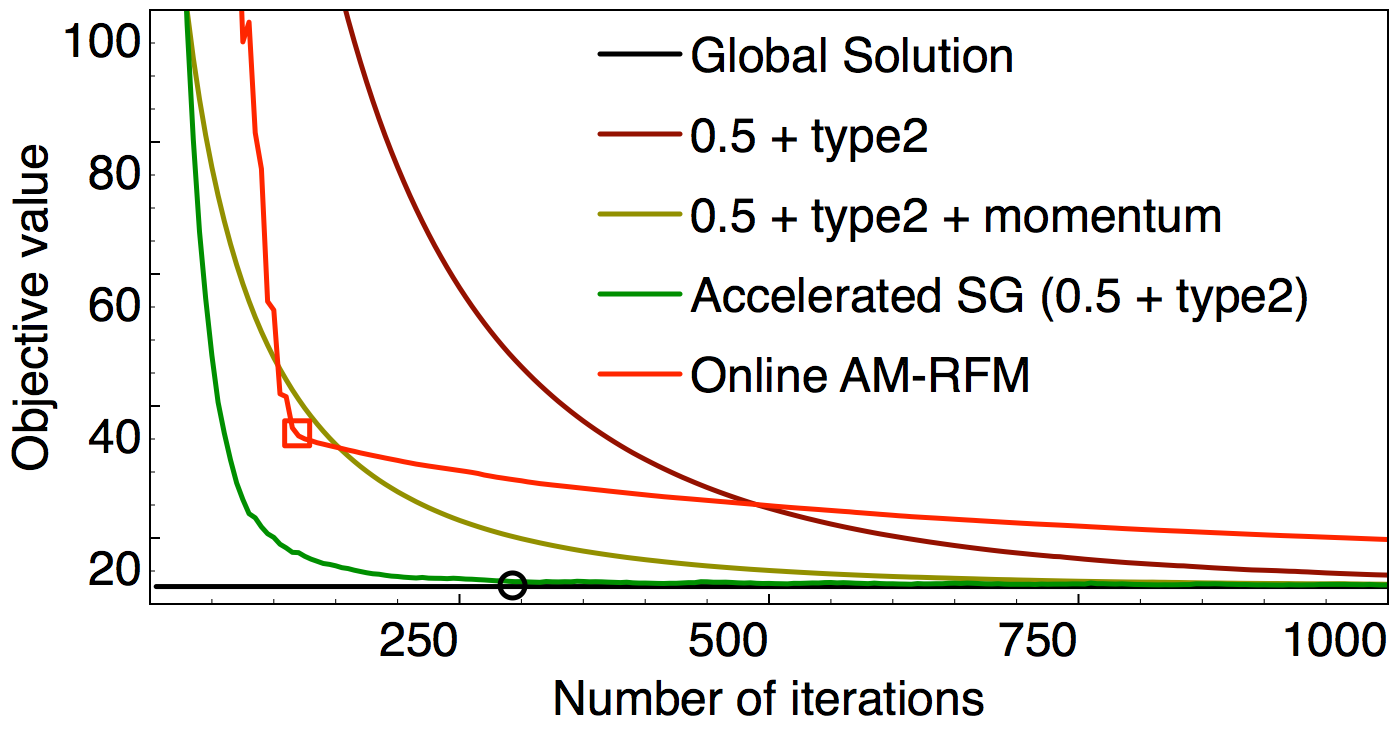
(c) Subspace

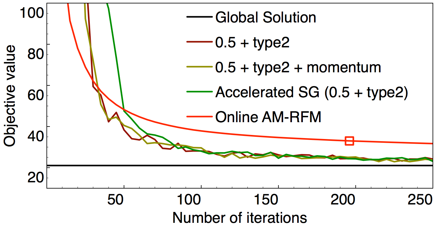
(d) Elastic net ($\nu_{\textrm{H}}=1.0,\nu_{\textrm{D}}=0.5$)

Figure 8: Comparison of different incremental algorithms for induced DLMs. The plots in (c) and (d) depict early learning for (a) and (b) respectively (i.e., they are zoomed into early learning in those plots). Accelerated SG is SGD AM-DLM  with $\eta_{t}=\eta_{t-1}$ if $\mathop{\mathrm{tr}}(\nabla l_{t}(\mathbf{D}_{t-1})^{\top}\nabla l_{t}(\mathbf{D}_{t-2}))\geq 0$ and otherwise selects $\eta_{t}=\eta_{0}/\sqrt{t}$ (type 2) or $\eta_{t}=\eta_{0}/t$ (type 3). For momentum, $\beta_{t}=0.01$. Both of these accelerations outperformed the best setting for standard SGD AM-DLM  (with $\eta_{0}=0.5$ and type 2 decay), for subspace dictionary learning. For elastic net, however, the accelerations appeared to have little impact, potentially due to the fact that convergence of the standard SGD AM-DLM  was already fast. A surprising observation is that online AM-DLM  decreases the function value very fast at the beginning, but then slows before converging to the global solution. Finally, we report the runtime of SGD AM-DLM. The two marks in each plots denote convergence and runtime information based on Accelerated SG. The black circle denotes the step where Accelerated SG is within 5% of the batch solution; the black square denotes the step where Accelerated SG spends as much cumulative time as the batch one. If a mark is missing in a plot, then the mark is beyond the maximum iterations. These black marks are similar for the other stochastic approaches. This convergence is within $30\%-40\%$ of the time needed for the global solution. This is a serious underestimate of the true gains of stochastic gradient descent, because $T=100$ was chosen to make the comparison to the global batch solution computationally feasible. In practice, this value is much larger and stochastic gradient descent becomes the obvious choice for estimating induced DLMs if efficiency is a concern. The red circle and square have the same meanings as the black ones except for that they are for online AM-DLM. In contrast to black marks, this convergence is more than 10 times of the time needed for the global solution, demonstrating that online AM-DLM  is computationally costly and slow convergence while it is sample efficient and with no need to select step-size explicitly.

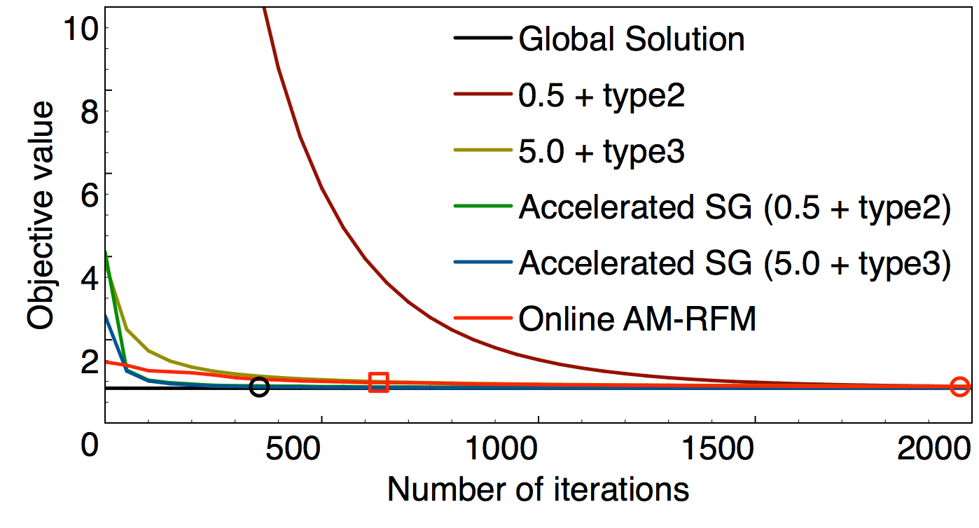
(a) Subspace

(b) Elastic net ($\nu_{\textrm{H}}=1.0,\nu_{\textrm{D}}=0.5$)

Figure 9: Comparison of different incremental algorithms for induced DLMs on data randomly drawn from the Extended Yale Face Database B, with $T=1000$ and $d=100$. All the settings are the same as in Figure 8 except for that the black marks are for Accelerated SG (5.0 + type3) rather than Accelerated SG (0.5 + type2). In this experiment, setting $\eta_{0}=5.0$ and using type 3 decay converges faster than setting $\eta_{0}=0.5$ and using type 2. Accelerated SG still accelerates SGD AM-DLM  in (a), and appears to have little impact in (b) where SGD AM-DLM  already converges fast. The methods with momentum term are not shown in the plots, because they are almost the same as or even a bit worse than the ones without momentum, denoting that adding momentum is not guaranteed to improve the convergence of the SGD algorithm. We also notice that online AM-DLM  always needs much more time to converge than all the stochastic methods, even though it converges within fewer steps. For example, in (b), the time needed for online AM-DLM  to reach the red circle is around 1400% of the time for Accelerated SG (5.0 + type3) to reach the black circle, where the solutions are within 5% of the batch solution, despite that the red circle is within much fewer steps than the black one.

7.3 Experimental results

In this section, we empirically investigate the properties of these incremental estimation strategies for induced DLMs. Previous sections indicated the global optimality of the alternating minimization for the batch setting; our goal in this section is to empirically demonstrate that this result holds for incremental estimation, and provide insight into which strategies are most effective for incremental estimation. In addition to online AM-DLM  and the accelerations to SGD AM-DLM, we explore more basic step-size selection strategies, including constant step-sizes and standard decay schedules. We include results for poorly selected step-sizes, and do not necessarily advocate for any one algorithm. Our goal is to provide preliminary insights into the incremental properties for induced DLMs, to make it simpler for others to practically select and use these algorithms.

The experiments compare the objective value of the incremental approaches to the global batch solution. At each iteration, the objective value for the current $\mathbf{D}$ is computed as

$$\alpha\sum_{i=1}^{k}\|\mathbf{D}_{:i}\|_{c}^{2}+\frac{1}{T}\min_{\mathbf{H}\in\mathbb{R}^{k\times T}}\sum_{t=1}^{T}\|\mathbf{D}\mathbf{H}_{:t}-\mathbf{X}_{:t}\|_{2}^{2}+\alpha\sum_{i=1}^{k}\|\mathbf{H}_{i:}\|_{r}^{2}.$$

The loss function is a least-squares loss, to enable comparison with online AM-DLM. The regularizer weight is $\alpha=0.05$, where the regularizer on $\mathbf{H}$ is appropriately scaled with the number of samples (as discussed in Section 3.3). The data is synthetically generated from a unit-variance Gaussian, with $d=50$ and $T=100$. A smaller $T$ was chosen to make it computationally feasible to run the batch algorithm, to give the global solution for comparison. The incremental algorithms iterate over the dataset multiple times, with a random reshuffling of data each time. The results are summarized in Figures 7, 8 and 9. Figure 7 investigates properties of fixed step-sizes and decay schedules for SGD AM-DLM. Figure 8 and 9 investigate the properties of all the algorithms, including SGD AM-DLM  with accelerations and online AM-DLM, on synthetic and real data.

The results are described more fully in the figure captions, but we provide the overall conclusions here. 1) SGD converges to a good solution much more efficiently than batch AM-DLM; 2) both accelerations to SGD AM-DLM  improve the convergence rate and 3) online AM-DLM converges in only a few epochs and is effective with line-search to select step-sizes, but is quite slow per step. The selection of step-sizes for SGD is not particularly sensitive, and even a relatively aggressive step size with decay converged after some oscillation. The step-size selection is even less sensitive with acceleration, because a more conservative list of step-sizes can be chosen. In this way, the algorithm can keep a larger step size for a number of steps until the sign changes and then pick a more conservative step-size from the list. However, if one wants to avoid picking a step-size and more memory and computation is available, online AM-DLM  is a reasonable alternative.

8 Related work

There has been a recent focus on understanding alternating minimization for problems in machine learning, and on effective strategies for escaping saddle points, particularly for neural networks. We summarize much of this work here, to better complete the emerging picture for strategies to optimize such biconvex objectives.

The most general and relevant related work is the treatise by Haeffele and Vidal (2015) on global optimality for a wide class of models, including dictionary learning models and neural networks with rectified linear activations. They show that when the solutions are rank-deficient, in their case specifically having a column of all zeros in their factors, that local minima are in fact global minima. This work complements the results in this paper, because we focused on the overcomplete setting, where the solution is not rank deficient. Other more specific global optimality results, that largely fit within the results by Haeffele and Vidal (2015), include a setting with a least-squares loss, unweighted trace norm and conditions on the value of the loss at the given stationary point (Mardani et al., 2013); an unregularized setting (Abernethy et al., 2009, Proposition 5); an online robust PCA setting where the true rank is assumed to be known (Feng et al., 2013); and a recent result on local minima for deep linear neural networks Kawaguchi (2016).

A common strategy in previous efforts to obtain global solutions for biconvex problems has been to provide careful initialization strategies and assume sparsity or coherence properties on the matrices. Jain et al. (2013) showed that alternating minimization for matrix completion provides global solutions, assuming that the given matrix and optimal factors are incoherent matrices (Jain et al., 2013, Definition 2.4), which enables them to define a suitable initial point using a singular value decomposition. Gunasekar et al. (2013) and Hardt (2014) further generalize these assumptions, particularly to the noisy setting and Netrapalli et al. (2015) to the setting for phase retrieval. For sparse coding, Spielman et al. (2012) showed how to recover the optimal dictionary exactly, assuming it has full column rank and assuming a maximum sparsity level on the basis. Since then, most work has focused on the overcomplete case, where the dictionary is not full column rank. Agarwal et al. (2017) showed that alternating minimization for sparse coding with thresholding gives global solutions, if the dictionary satisfies the restricted isometry property Candès and Tao (2005) and using a provable strategy to initialize the dictionary to be near optimal. Previously, both Agarwal et al. (2017) and Arora et al. (2014) had independently provided a similar algorithm, with incoherence requirements on the matrices, with slightly different requirements on the sparsity level. Arora et al. (2015) built on this work and expanded the level of possible sparsity.

A separate line of work has required fewer assumptions on the true matrices and pursued initialization strategies by generating candidate columns, typically using singular value decompositions d’Aspremont et al. (2004); Bach et al. (2008); Journée et al. (2010); Zhang et al. (2012); Mirzazadeh et al. (2015). The bulk of this work has been on the semi-definite case, including seminal work by Burer and Monteiro (2005), where the two factors are the same, $\mathbf{Z}=\mathbf{D}\mathbf{D}^{\top}$. The exception is the GCG algorithm Zhang et al. (2012); Yu et al. (2014), which generates columns and rows for $\mathbf{D}$ and $\mathbf{H}$ for some of the induced DLMs considered in this work. Though the boosting algorithm is quite general, it requires an oracle solution for a problem that is intractable except for in a small number of cases, which mostly correspond to those with known induced regularizers. Most of this work has not characterized the saddle-points of the non-convex optimization, with the exception of a recent work for the semi-definite setting which identified a smoothness condition on the gradient of the loss that ensured convergence to global solutions (Mirzazadeh et al., 2015, Proposition 2). The results in this work suggest that it is likely unnecessary to carefully generate candidate columns and rows, though for large $d$, progressively increasing $k$ could be computationally attractive.

Another strategy has been to use the convex reformulations obtained for induced DLMs. For example, instead of alternating on $\mathbf{D}$ and $\mathbf{H}$ in the subspace formulation, $\mathbf{Z}$ is solved for directly in trace norm regularized problem. From there, the factors $\mathbf{D}$ and $\mathbf{H}$ could typically be recovered, usually with iterative methods. The problems tackled with this approach include relaxed rank exponential family PCA Bach et al. (2008); Zhang et al. (2011), matrix completion Cai et al. (2010), (semi-)supervised dictionary learning Goldberg et al. (2010); Zhang et al. (2011), multi-view learning White et al. (2012), co-embedding Mirzazadeh et al. (2014) and autoregressive moving average models White et al. (2015). These approaches, however, are often not as scalable as learning the factors $\mathbf{D}$ and $\mathbf{H}$, which can be smaller. Further, because $\mathbf{Z}$ grows with the size of the data, and the induced regularizer often couples entries across $\mathbf{Z}$, the induced convex reformulation is typically not amenable to incremental estimation. As an additional problem, for the general class of induced DLMs, the induced convex formulation is only of theoretical value, since there is no known form for the induced norm and so the optimization over $\mathbf{Z}$ cannot be performed. There has been some effort to obtain approximations to the convex form for the elastic net, which does not have a known induced form (Bach et al., 2008); the proposed approach, however, uses a convex lower bound and the relation to the elastic net solution is unclear. The alternating minimization approach avoids the need to have an explicit form for the induced norm, and rather only uses the property that this class has induced forms to identify promising situations for global optimality.

For incremental estimation of induced DLMs, there are significantly fewer approaches. Outside of incremental principal components analysis Warmuth and Kuzmin (2008); Feng et al. (2013) and partial least-squares Arora et al. (2012), little is known about how to obtain optimal incremental DLM  estimation and several approaches have settled for local solutions Mairal et al. (2009a, b, 2010). De Sa et al. (2015) prove convergence to a global solution, with random initialization, using incremental, stochastic gradient descent algorithms for an interesting subset of induced DLMs, including for matrix completion, phase retrieval and subspace tracking. These problems, however, are formulated as semi-definite problems, again by learning $\mathbf{Z}=\mathbf{D}\mathbf{D}^{\top}$. The incremental estimation results in this work apply to a broader class of models—induced DLMs— and provide justification for a simple descent approach with stochastic gradient descent.

9 Conclusion and Discussion

In this work, we addressed tractable estimation of induced dictionary learning models (DLMs), which constitute a broad and widely used formalism for unsupervised, semi-supervised and supervised learning problems. We generalized the class of induced DLMs and provided several new objectives and characterizations of stationary points. We proved that local minima are global minima for a subclass of induced DLMs and showed that there are no degenerate saddlepoints for one setting. Further, we empirically demonstrated that alternating minimization results in global minima for an even broader class. Motivated by these insights, we then empirically investigated the practical estimation properties of simple alternating minimization algorithms, particularly for incremental estimation. The main theoretical novelty in this work is to characterize the stationary points where the learned factors are full rank, as opposed to the rank-deficient setting which has been more thoroughly characterized.

A key insight from this paper is that that we can identify tractable dictionary learning objectives using the class of induced DLMs. For those dictionary learning methods that can be specified as induced DLMs, we provide compelling evidence that local minima are global minima and, in some cases, that there are no degenerate saddlepoints. Consequently, a simple alternating minimization scheme is effective for obtaining global solutions. To be more precise, we show a general result for the optimality of stationary points for the induced form, and highlight a necessary condition—the induced regularization property—to prove a similar result for the factored form. We then show one setting that satisfies the induced regularization property, i.e., for the case of strictly convex regularizers and Holder continuous losses. These general results provide insights into specific settings of interest, showing that local minima are global minima for

1. matrix completion using squared regularizers on the factors, with any invertible weighting on the squared regularizer on $\mathbf{D}$, where the inner dimension $k$ can be set less than $d$ (Theorem 11)

2. sparse coding with a pseudo-Huber smooth approximation to the $\ell_{1}$ regularizer, for sufficiently large $k$ (Corollary 10)

3. dictionary learning with the elastic net on either $\mathbf{D}$ and $\mathbf{H}$, where again the $\ell_{1}$ regularizer is approximated with the pseudo-Huber function and $k$ is sufficiently large (Corollary 10).

The result is proved for the more general class of induced DLMs, as opposed to previous results which were proved for each specific setting. Therefore, though the results from this paper provide novel insights for each of these specific settings, the larger contribution is to provide a new proof strategy for characterizing stationary points of dictionary learning methods.

The generality of this result, however, is limited in two important ways. First, to characterize saddlepoints using directional derivatives, we have assumed that the losses and regularizers are differentiable. Consequently, the results do not directly apply to standard sparse regularizers, such as $\ell_{1}$. Nonetheless, they do apply to smooth approximations, such as the pseudo-Huber smooth approximation. The pseudo-Huber function has a parameter $\sigma$; when $\sigma\rightarrow 0$, the pseudo-Huber approaches $\ell_{1}$. The results in this paper apply to arbitrarily small $\sigma$; a limit argument should extend the results to these non-smooth regularizers. An important next step, therefore, is to formally characterize this intuition, so that these results directly apply to settings such as sparse coding.

A second limitation is that the results do not yet provide a precise specification for the inner dimension, $k$. The proof requires $k$ to be large enough, to ensure that $\mathrm{R}_{k}$ is convex. We know that for $k$ at least as large as the true induced dimension, then $\mathrm{R}_{k}$ is equal to the induced regularizer ${\mathrm{R}_{\mathrm{\scriptsize Z}}}$ which is guaranteed to be convex. For smaller $k$, however, $\mathrm{R}_{k}$ could still be convex, or potentially have nice properties such as pseudo-convexity. The increase of $k$ has a diminishing returns property, and we expect $\mathrm{R}_{k}$ to behave similarly to ${\mathrm{R}_{\mathrm{\scriptsize Z}}}$ before $k$ actually reaches the magnitude of the true induced dimension. In fact, we find that $k$ can be quite a bit smaller than the true induced dimension and alternating minimization still provides global solutions. We hypothesize that this is in fact because $\mathrm{R}_{k}$ even for small $k$ is already close to being a convex function (e.g., it could be pseudoconvex). To provide an even more general result, and to characterize what we see in practice, a useful direction would be to extend the proof to pseudo-convex induced regularizers and to investigate specific choices of regularizers and $k$ that produce pseudo-convex induced regularizers.

A Additional information about regularizers

Proposition 12

For any $m$ non-negative convex functions $g_{i}:\mathbb{R}^{d}\rightarrow\mathbb{R}^{+}$, $g(\mathbf{d})=\sqrt{g_{1}^{2}(\mathbf{d})+\ldots g_{m}^{2}(\mathbf{d})}$ is convex. Further, if the $g_{i}$ are all norms, then $g$ is a norm.

Proof:  Notice that $g$ can be seen as the composition of the $\ell_{2}$ norm on the vector of $m$ values of $g_{i}$ applied to $\mathbf{d}$. We can use the convexity properties of both to obtain the result. Take any $\eta\in[0,1]$ and any $\mathbf{a},\mathbf{b}\in\mathbb{R}^{d}$.

$$g(\eta\mathbf{a}+(1-\eta)\mathbf{b}) =\ell_{2}([g_{1}(\eta\mathbf{a}+(1-\eta)\mathbf{b}),\ldots,g_{m}(\eta\mathbf{a}+(1-\eta)\mathbf{b})])$$

$$\leq\ell_{2}([\eta g_{1}(\mathbf{a})+(1-\eta)g_{1}(\mathbf{b}),\ldots,\eta g_{m}(\mathbf{a})+(1-\eta)g_{m}(\mathbf{b})])$$

$$=\ell_{2}(\eta[g_{1}(\mathbf{a}),\ldots,g_{m}(\mathbf{a})]+(1-\eta)[g_{1}(\mathbf{b}),\ldots,g_{m}(\mathbf{b})])$$

$$\leq\eta\ell_{2}([g_{1}(\mathbf{a}),\ldots,g_{m}(\mathbf{a})])+(1-\eta)\ell_{2}([g_{1}(\mathbf{b}),\ldots,g_{m}(\mathbf{b})])$$

$$=\eta g(\mathbf{a})+(1-\eta)g(\mathbf{b})$$

The first inequality follows from the fact that $\ell_{2}$ is monotonically increasing on the set of non-negative values and the $g_{i}$ are all non-negative, so for any $\mathbf{d}\in\mathbb{R}^{d}$, $b\in\mathbb{R}^{+}$ such that, $g_{i}(\mathbf{d})\leq b$ implies $g_{i}^{2}(\mathbf{d})\leq b^{2}$. Therefore, $g$ is convex.

If the $g_{i}$ are norms, then clearly $g$ satisfies absolute homogeneity $g(\eta\mathbf{d})=\eta g(\mathbf{d})$ and $g(\mathbf{d})=0$ implies $\mathbf{d}=\mathbf{\bm{0}}$. The triangle inequality follows similarly to above, obtained by setting $\eta=0.5$ and using the absolute homogeneity of $g$. $\hbox{}\hfill\blacksquare$

We can use this result to use separate norms on different parts of the columns or rows of $\mathbf{D}$ and $\mathbf{H}$. This is particularly useful for supervised learning, where $\mathbf{D}$ is partitioned into two components, one for the unsupervised recovery and the other for supervised learning.

Corollary 13

For some $m<d$ with two functions $g_{1}:\mathbb{R}^{m}\rightarrow\mathbb{R}^{+}$ and $g_{2}:\mathbb{R}^{d-m}\rightarrow\mathbb{R}^{+}$ which act on the two partitions of $\mathbf{d}\in\mathbb{R}^{d}$, the regularizer $g(\mathbf{d})=\sqrt{g_{1}^{2}(\mathbf{d}_{1:m})+g_{2}^{2}(\mathbf{d}_{(m+1):d})}$ is a convex, non-negative function in $\mathbb{R}^{d}$.

Proof:  We can extend both functions $g_{1}$ and $g_{2}$ to the domain $\mathbb{R}^{d}$, simply by having those parts not influence the function value. These extended functions are still non-negative, and so satisfy the conditions of Proposition 12. The function $g$ defined with the extended functions is exactly the same, and so we obtain the desired result. $\hbox{}\hfill\blacksquare$

B Proof of Global Optimality for Weighted Frobenius Norm

We prove the result for Theorem 11 in this section. We do so by proving the more general results in Theorem 14, where in the main text we presented a simpler statement that highlighted the properties of saddlepoints.

We consider a general optimization, with a row weighting ${\bm{\Lambda}}$ on $\mathbf{D}$.

$$\min_{\mathbf{D}\in\mathbb{R}^{d\times k},\mathbf{H}\in\mathbb{R}^{k\times T}}\mathrm{L}(\mathbf{D}\mathbf{H})+\tfrac{\alpha}{2}\left\|{\bm{\Lambda}}\mathbf{D}\right\|_{F}^{2}+\tfrac{\alpha}{2s^{2}}\left\|\mathbf{H}\right\|_{F}^{2}$$

Without loss of generality, we can adjust the diagonal weighting ${\bm{\Lambda}}$, and avoid the cluttered additional weighting using $s^{2}$. This can be done by setting $\alpha=\frac{\alpha_{\text{original}}}{s^{2}}$ and ${\bm{\Lambda}}=s^{2}{\bm{\Lambda}}_{\text{original}}$. We do not absorb $\alpha$ into ${\bm{\Lambda}}$, because for simplicity of the proof, we require an invertible ${\bm{\Lambda}}$, but allow $\alpha=0$ to cover the unregularized setting.

Theorem 14

For invertible ${\bm{\Lambda}}\in\mathbb{R}^{d\times d}$ and $\alpha\geq 0$, let $(\bar{\mathbf{D}},\bar{\mathbf{H}})$ be a stationary point of

$$\min_{\mathbf{D}\in\mathbb{R}^{d\times k},\mathbf{H}\in\mathbb{R}^{k\times T}}\mathrm{L}(\mathbf{D}\mathbf{H})+\tfrac{\alpha}{2}\left\|{\bm{\Lambda}}\mathbf{D}\right\|_{F}^{2}+\tfrac{\alpha}{2}\left\|\mathbf{H}\right\|_{F}^{2}$$ (24)

If either

1. $\|{\bm{\Lambda}}^{-\top}\nabla\mathrm{L}(\bar{\mathbf{D}}\bar{\mathbf{H}})\|_{2}\leq\alpha$ (i.e., the maximum singular value is $\alpha$); or

2. the Hessian is positive semi-definite with $(\bar{\mathbf{D}},\bar{\mathbf{H}})$ rank-deficient

then $\mathbf{Z}=\bar{\mathbf{D}}\bar{\mathbf{H}}$ is a globally optimal solution to

$$\mathop{\mathrm{argmin}}_{\mathbf{Z}\in\mathbb{R}^{d\times T}}\mathrm{L}(\mathbf{Z})+\alpha\left\|{\bm{\Lambda}}\mathbf{Z}\right\|_{tr}.$$ (26)

Proof: 

Since $\bar{\mathbf{D}}$ and $\bar{\mathbf{H}}$ are stationary points of (24), we know

$$\nabla_{\mathbf{D}}=\nabla\mathrm{L}(\bar{\mathbf{D}}\bar{\mathbf{H}})\bar{\mathbf{H}}^{\top}+\alpha{\bm{\Lambda}}^{\top}{\bm{\Lambda}}\bar{\mathbf{D}}=\mathbf{\bm{0}}$$ (27)

$$\nabla_{\mathbf{H}}=\bar{\mathbf{D}}^{\top}\nabla\mathrm{L}(\bar{\mathbf{D}}\bar{\mathbf{H}})+\alpha\bar{\mathbf{H}}=\mathbf{\bm{0}}$$ (28)

By multiplying both sides by $\bar{\mathbf{D}}^{\top}$ or $\bar{\mathbf{H}}^{\top}$ respectively, and taking the trace, we get

$$\mathop{\mathrm{tr}}\left(\nabla\mathrm{L}(\bar{\mathbf{D}}\bar{\mathbf{H}})\bar{\mathbf{H}}^{\top}\bar{\mathbf{D}}^{\top}\right)+\alpha\mathop{\mathrm{tr}}\left({\bm{\Lambda}}^{\top}{\bm{\Lambda}}\bar{\mathbf{D}}\bar{\mathbf{D}}^{\top}\right)=\mathbf{\bm{0}}$$ (29)

$$\mathop{\mathrm{tr}}\left(\bar{\mathbf{H}}^{\top}\bar{\mathbf{D}}^{\top}\nabla\mathrm{L}(\bar{\mathbf{D}}\bar{\mathbf{H}})\right)+\alpha\mathop{\mathrm{tr}}\left(\bar{\mathbf{H}}^{\top}\bar{\mathbf{H}}\right)=\mathbf{\bm{0}}$$ (30)

Now, we know that the trace norm can be characterized as follows (Recht et al., 2010)

$$\left\|\mathbf{Z}\right\|_{tr} =\min_{\mathbf{W}_{1},\mathbf{W}_{2}}\tfrac{1}{2}\mathop{\mathrm{tr}}\left(\mathbf{W}_{1}\right)+\tfrac{1}{2}\mathop{\mathrm{tr}}\left(\mathbf{W}_{2}\right)\text{ s.t. }\mathbf{W}=\left(\begin{array}[]{cc}\mathbf{W}_{1}&\mathbf{Z}\\ \mathbf{Z}^{\top}&\mathbf{W}_{2}\end{array}\right)\succeq 0$$

giving weighted norm

$$\left\|{\bm{\Lambda}}\mathbf{Z}\right\|_{tr} =\min_{\mathbf{W}_{1},\mathbf{W}_{2}}\tfrac{1}{2}\mathop{\mathrm{tr}}\left(\mathbf{W}_{1}\right)+\tfrac{1}{2}\mathop{\mathrm{tr}}\left(\mathbf{W}_{2}\right)\text{ s.t. }\mathbf{W}=\left(\begin{array}[]{cc}\mathbf{W}_{1}&{\bm{\Lambda}}\mathbf{Z}\\ \mathbf{Z}^{\top}{\bm{\Lambda}}^{\top}&\mathbf{W}_{2}\end{array}\right)\succeq 0$$

A Lagrange multiplier $\mathbf{M}\in\mathbb{R}^{(d+T)\times(d+T)}$ can be used to bring the constraint $\mathbf{W}\succeq 0$ into the objective and consider the Lagrangian with $\mathbf{M}\succeq 0$:

$$\mathcal{L}(\mathbf{Z},\mathbf{W}_{1},\mathbf{W}_{2},\mathbf{M}) =\mathrm{L}(\mathbf{Z})+\tfrac{\alpha}{2}\mathop{\mathrm{tr}}\left(\mathbf{W}_{1}\right)+\tfrac{\alpha}{2}\mathop{\mathrm{tr}}\left(\mathbf{W}_{2}\right)-\mathop{\mathrm{tr}}\left(\mathbf{M}^{\top}\mathbf{W}\right)$$ (31)

Notice first that, writing $\mathbf{M}$ in a block structure,

$$\mathbf{W}^{\top}\mathbf{M}=\left(\begin{array}[]{cc}\mathbf{W}_{1}^{\top}&{\bm{\Lambda}}\mathbf{Z}\\ \mathbf{Z}^{\top}{\bm{\Lambda}}^{\top}&\mathbf{W}_{2}^{\top}\end{array}\right)\left(\begin{array}[]{cc}\mathbf{M}_{1}&\mathbf{M}_{2}\\ \mathbf{M}_{3}&\mathbf{M}_{4}\end{array}\right)=\left(\begin{array}[]{cc}\mathbf{W}_{1}^{\top}\mathbf{M}_{1}+{\bm{\Lambda}}\mathbf{Z}\mathbf{M}_{3}&\mathbf{W}_{1}^{\top}\mathbf{M}_{2}+{\bm{\Lambda}}\mathbf{Z}\mathbf{M}_{4}\\ \mathbf{Z}^{\top}{\bm{\Lambda}}^{\top}\mathbf{M}_{1}+\mathbf{W}_{2}^{\top}\mathbf{M}_{3}&\mathbf{Z}^{\top}{\bm{\Lambda}}^{\top}\mathbf{M}_{2}+\mathbf{W}_{2}^{\top}\mathbf{M}_{4}\\ \end{array}\right)$$

we get $\mathop{\mathrm{tr}}\left(\mathbf{M}^{\top}\mathbf{W}\right)=\mathop{\mathrm{tr}}\left(\mathbf{W}^{\top}\mathbf{M}\right)=\mathop{\mathrm{tr}}\left(\mathbf{W}_{1}^{\top}\mathbf{M}_{1}\right)+\mathop{\mathrm{tr}}\left({\bm{\Lambda}}\mathbf{Z}\mathbf{M}_{3}\right)+\mathop{\mathrm{tr}}\left(\mathbf{Z}^{\top}{\bm{\Lambda}}^{\top}\mathbf{M}_{2}\right)+\mathop{\mathrm{tr}}\left(\mathbf{W}_{2}^{\top}\mathbf{M}_{4}\right)$.

The KKT conditions for this optimization require

Gradient conditions:

$$\nabla\mathcal{L}(\mathbf{Z},\mathbf{W}_{1},\mathbf{W}_{2},\mathbf{M})=\nabla\mathrm{L}(\mathbf{Z})-{\bm{\Lambda}}^{\top}\mathbf{M}_{3}^{\top}-{\bm{\Lambda}}^{\top}\mathbf{M}_{2}=\mathbf{\bm{0}}$$ (32)

$$\nabla_{\mathbf{W}_{1}}\mathcal{L}(\mathbf{Z},\mathbf{W}_{1},\mathbf{W}_{2},\mathbf{M})=\tfrac{\alpha}{2}\mathbf{I}_{d}-\mathbf{M}_{1}=\mathbf{\bm{0}}$$ (33)

$$\nabla_{\mathbf{W}_{2}}\mathcal{L}(\mathbf{Z},\mathbf{W}_{1},\mathbf{W}_{2},\mathbf{M})=\tfrac{\alpha}{2}\mathbf{I}_{T}-\mathbf{M}_{4}=\mathbf{\bm{0}}$$ (34)

Complementary slackness:

$$\mathop{\mathrm{tr}}\left(\mathbf{M}^{\top}\mathbf{W}\right)=0$$ (35)

Primal feasibility:

$$\mathbf{W}\succeq 0$$ (36)

Dual feasibility:

$$\mathbf{M}\succeq 0$$ (37)

We introduce candidate variables using the stationary points $\bar{\mathbf{D}}$ and $\bar{\mathbf{H}}$ of the nonconvex objective (24): $\mathbf{Z}=\bar{\mathbf{D}}\bar{\mathbf{H}}$, $\mathbf{W}_{1}={\bm{\Lambda}}\bar{\mathbf{D}}\bar{\mathbf{D}}^{\top}{\bm{\Lambda}}^{\top}$, $\mathbf{W}_{2}=\bar{\mathbf{H}}^{\top}\bar{\mathbf{H}}$, $\mathbf{M}_{1}=\tfrac{\alpha}{2}\mathbf{I}_{d}$, $\mathbf{M}_{4}=\tfrac{\alpha}{2}\mathbf{I}_{T}$, $\mathbf{M}_{2}=\tfrac{1}{2}{\bm{\Lambda}}^{-\top}\nabla\mathrm{L}(\mathbf{Z})$ and $\mathbf{M}_{3}=\mathbf{M}_{2}^{\top}$.

These variables clearly satisfy all the gradient conditions. Complementary slackness holds since

$$\mathop{\mathrm{tr}}\left(\mathbf{M}^{\top}\mathbf{W}\right)=\mathop{\mathrm{tr}}\left({\bm{\Lambda}}\bar{\mathbf{D}}\bar{\mathbf{D}}^{\top}{\bm{\Lambda}}^{\top}\tfrac{\alpha}{2}\mathbf{I}_{d}\right)+\mathop{\mathrm{tr}}\left({\bm{\Lambda}}\bar{\mathbf{D}}\bar{\mathbf{H}}\tfrac{1}{2}\nabla\mathrm{L}(\mathbf{Z})^{\top}{\bm{\Lambda}}^{-1}\right)+$$

$$\hskip 85.35826pt\mathop{\mathrm{tr}}\left(\bar{\mathbf{H}}^{\top}\bar{\mathbf{D}}^{\top}{\bm{\Lambda}}^{\top}\tfrac{1}{2}{\bm{\Lambda}}^{-\top}\nabla\mathrm{L}(\mathbf{Z})\right)+\mathop{\mathrm{tr}}\left(\bar{\mathbf{H}}^{\top}\bar{\mathbf{H}}\tfrac{\alpha}{2}\mathbf{I}_{T}\right)$$

$$=\tfrac{\alpha}{2}\mathop{\mathrm{tr}}\left({\bm{\Lambda}}\bar{\mathbf{D}}\bar{\mathbf{D}}^{\top}{\bm{\Lambda}}^{\top}\right)+\tfrac{1}{2}\mathop{\mathrm{tr}}\left(\bar{\mathbf{D}}\bar{\mathbf{H}}\nabla\mathrm{L}(\mathbf{Z})^{\top}\right)+\tfrac{1}{2}\mathop{\mathrm{tr}}\left(\bar{\mathbf{H}}^{\top}\bar{\mathbf{D}}^{\top}\nabla\mathrm{L}(\mathbf{Z})\right)+\tfrac{\alpha}{2}\mathop{\mathrm{tr}}\left(\bar{\mathbf{H}}^{\top}\bar{\mathbf{H}}\right)$$

$$=0$$

because of (29) and (30) and because the trace satisfies a circular property, $\mathop{\mathrm{tr}}\left(\mathbf{A}\mathbf{B}\mathbf{C}\right)=\mathop{\mathrm{tr}}\left(\mathbf{B}\mathbf{C}\mathbf{A}\right)=\mathop{\mathrm{tr}}\left(\mathbf{C}\mathbf{A}\mathbf{B}\right)$ and equality under transpose, $\mathop{\mathrm{tr}}\left(\mathbf{A}\right)=\mathop{\mathrm{tr}}\left(\mathbf{A}^{\top}\right)$.

To show primal feasibility, notice that

$$\mathbf{W}=\left(\begin{array}[]{cc}{\bm{\Lambda}}\bar{\mathbf{D}}\bar{\mathbf{D}}^{\top}{\bm{\Lambda}}^{\top}&{\bm{\Lambda}}\bar{\mathbf{D}}\bar{\mathbf{H}}\\ \bar{\mathbf{H}}^{\top}\bar{\mathbf{D}}^{\top}{\bm{\Lambda}}^{\top}&\bar{\mathbf{H}}^{\top}\bar{\mathbf{H}}\end{array}\right)=\left(\begin{array}[]{c}{\bm{\Lambda}}\bar{\mathbf{D}}\\ \bar{\mathbf{H}}^{\top}\end{array}\right)\left(\begin{array}[]{c}{\bm{\Lambda}}\bar{\mathbf{D}}\\ \bar{\mathbf{H}}^{\top}\end{array}\right)^{\top}\succeq 0$$

To show dual feasibility, we can use the Schur complement condition of block matrices: $\mathbf{M}\succeq 0$ iff $\mathbf{M}_{1}\succ 0$ and $\mathbf{M}_{4}-\mathbf{M}_{3}\mathbf{M}_{1}^{-1}\mathbf{M}_{2}\succeq 0$. Clearly, $\mathbf{M}_{1}=\tfrac{\alpha}{2}\mathbf{I}_{d}\succ 0$, since $\alpha>0$. Now,

$$\mathbf{M}_{4}-\mathbf{M}_{3}\mathbf{M}_{1}^{-1}\mathbf{M}_{2} =\tfrac{\alpha}{2}\mathbf{I}_{T}-\tfrac{1}{2}\nabla\mathrm{L}(\mathbf{Z})^{\top}{\bm{\Lambda}}^{-1}(\tfrac{\alpha}{2}\mathbf{I}_{d})^{-1}\tfrac{1}{2}{\bm{\Lambda}}^{-\top}\nabla\mathrm{L}(\mathbf{Z})$$

$$=\tfrac{\alpha}{2}\mathbf{I}_{T}-\tfrac{1}{2\alpha}\nabla\mathrm{L}(\mathbf{Z})^{\top}{\bm{\Lambda}}^{-1}{\bm{\Lambda}}^{-\top}\nabla\mathrm{L}(\mathbf{Z})$$

Case 1: general stationary point.

For $\alpha>0$, if $\|{\bm{\Lambda}}^{\raisebox{0.60275pt}{$\scriptscriptstyle-1$}}\nabla\mathrm{L}(\mathbf{Z})\|_{2}\leq\alpha$, then

$$\nabla\mathrm{L}(\mathbf{Z})^{\top}{\bm{\Lambda}}^{-1}{\bm{\Lambda}}^{-\top}\nabla\mathrm{L}(\mathbf{Z})\preceq\alpha^{2}\mathbf{I}$$

$$\implies\alpha^{2}\mathbf{I}_{T}-\nabla\mathrm{L}(\mathbf{Z})^{\top}{\bm{\Lambda}}^{-1}{\bm{\Lambda}}^{-\top}\nabla\mathrm{L}(\mathbf{Z})\succeq 0$$

$$\implies\tfrac{\alpha}{2}\mathbf{I}_{T}-\tfrac{1}{2\alpha}\nabla\mathrm{L}(\mathbf{Z})^{\top}{\bm{\Lambda}}^{-1}{\bm{\Lambda}}^{-\top}\nabla\mathrm{L}(\mathbf{Z})\succeq 0.$$

satisfying the dual feasibility requirement for this case.

If $\alpha=0$, then $\|{\bm{\Lambda}}^{\raisebox{0.60275pt}{$\scriptscriptstyle-1$}}\nabla\mathrm{L}(\mathbf{Z})\|_{2}\leq 0$, and so $\nabla\mathrm{L}(\mathbf{Z})=\mathbf{\bm{0}}$, again indicating $\mathbf{Z}=\bar{\mathbf{D}}\bar{\mathbf{H}}$ is a global optimum.

Case 2: rank-deficient stationary point has a positive semi-definite Hessian.

We will take advantage of the fact that the bottom $k-r$ singular values of $\bar{\mathbf{D}}$ and $\bar{\mathbf{H}}$ are zero. To conveniently write the Hessian for matrix-valued variables, we will use the directional derivative

$$D_{\mathbf{Y}}g(\mathbf{Y}_{0})[d\mathbf{Y}]=\lim_{t\rightarrow 0}\frac{g(\mathbf{Y}_{0}+td\mathbf{Y})-g(\mathbf{Y}_{0})}{t}=\langle\nabla_{\mathbf{Y}}g(\mathbf{Y}_{0}),d\mathbf{Y}\rangle$$

where $\langle\mathbf{A},\mathbf{B}\rangle=\mathop{\mathrm{tr}}(\mathbf{A}^{\top}\mathbf{B})$. For the Hessian, we get

$$D^{2}_{\mathbf{Y}}g(\mathbf{Y}_{0})[d\mathbf{Y},d\mathbf{Y}]=D_{\mathbf{Y}}\langle\nabla_{\mathbf{Y}}g(\mathbf{Y}_{0}),d\mathbf{Y}\rangle[d\mathbf{Y}]=\langle\nabla_{\mathbf{Y}}\langle\nabla_{\mathbf{Y}}g(\mathbf{Y}_{0}),d\mathbf{Y}\rangle,d\mathbf{Y}\rangle.$$

In our setting, $\mathbf{Y}_{0}=[\bar{\mathbf{D}};\bar{\mathbf{H}}^{\top}]\in\mathbb{R}^{(d+T)\times k}$ and $g([\bar{\mathbf{D}};\bar{\mathbf{H}}^{\top}])=\mathrm{L}(\bar{\mathbf{D}}\bar{\mathbf{H}})+\tfrac{\alpha}{2}\left\|{\bm{\Lambda}}\bar{\mathbf{D}}\right\|_{F}^{2}+\tfrac{\alpha}{2}\left\|\bar{\mathbf{H}}\right\|_{F}^{2}$. Let $\mathbf{G}=\nabla\mathrm{L}(\mathbf{Z})$ for $\mathbf{Z}=\bar{\mathbf{D}}\bar{\mathbf{H}}$, giving

$$D_{\mathbf{Y}}g(\mathbf{Y}_{0})[d\mathbf{Y}] =\left\langle\Bigl{[}\negthinspace\begin{smallmatrix}\mathbf{G}\bar{\mathbf{H}}^{\top}+\alpha{\bm{\Lambda}}^{\top}{\bm{\Lambda}}\bar{\mathbf{D}}\\ \mathbf{G}^{\top}\bar{\mathbf{D}}+\alpha\bar{\mathbf{H}}^{\top}\end{smallmatrix}\Bigr{]},\Bigl{[}\negthinspace\begin{smallmatrix}d\mathbf{D}\\ d\mathbf{H}^{\top}\end{smallmatrix}\Bigr{]}\right\rangle$$

$$=\mathop{\mathrm{tr}}(\bar{\mathbf{H}}\mathbf{G}^{\top}d\mathbf{D})+\alpha\mathop{\mathrm{tr}}(\bar{\mathbf{D}}^{\top}{\bm{\Lambda}}^{\top}{\bm{\Lambda}}d\mathbf{D})+\mathop{\mathrm{tr}}(\bar{\mathbf{D}}^{\top}\mathbf{G}d\mathbf{H}^{\top})+\alpha\mathop{\mathrm{tr}}(\bar{\mathbf{H}}d\mathbf{H}^{\top}).$$

Similarly, for the Hessian,

$$D^{2}_{\mathbf{Y}}g(\mathbf{Y}_{0})[d\mathbf{Y},d\mathbf{Y}] =\left\langle\nabla_{\mathbf{Y}}\left(\mathop{\mathrm{tr}}(\bar{\mathbf{H}}\mathbf{G}^{\top}d\mathbf{D})+\alpha\mathop{\mathrm{tr}}(\bar{\mathbf{D}}^{\top}{\bm{\Lambda}}^{\top}{\bm{\Lambda}}d\mathbf{D})+\mathop{\mathrm{tr}}(\bar{\mathbf{D}}^{\top}\mathbf{G}d\mathbf{H}^{\top})+\alpha\mathop{\mathrm{tr}}(\bar{\mathbf{H}}d\mathbf{H}^{\top})\right),d\mathbf{Y}\right\rangle$$

$$=\left\langle\Bigl{[}\negthinspace\begin{smallmatrix}\alpha{\bm{\Lambda}}^{\top}{\bm{\Lambda}}d\mathbf{D}+\mathbf{G}d\mathbf{H}^{\top}\\ \mathbf{G}^{\top}d\mathbf{D}+\alpha d\mathbf{H}^{\top}\end{smallmatrix}\Bigr{]},\Bigl{[}\negthinspace\begin{smallmatrix}d\mathbf{D}\\ d\mathbf{H}^{\top}\end{smallmatrix}\Bigr{]}\right\rangle+D^{2}_{\mathbf{Z}}\mathrm{L}(\mathbf{Z})[\bar{\mathbf{D}}d\mathbf{H}+d\mathbf{D}\bar{\mathbf{H}},\bar{\mathbf{D}}d\mathbf{H}+d\mathbf{D}\bar{\mathbf{H}}]$$

$$=2\mathop{\mathrm{tr}}(d\mathbf{D}^{\top}\mathbf{G}d\mathbf{H}^{\top})+\alpha\mathop{\mathrm{tr}}(d\mathbf{D}^{\top}{\bm{\Lambda}}^{\top}{\bm{\Lambda}}d\mathbf{D})+\alpha\mathop{\mathrm{tr}}(d\mathbf{H}^{\top}d\mathbf{H})$$

$$\hskip 28.45274pt+D^{2}_{\mathbf{Z}}\mathrm{L}(\mathbf{Z})[\bar{\mathbf{D}}d\mathbf{H}+d\mathbf{D}\bar{\mathbf{H}},\bar{\mathbf{D}}d\mathbf{H}+d\mathbf{D}\bar{\mathbf{H}}].$$

Now we can make the last term, the Hessian w.r.t. $\mathrm{L}$, disappear by carefully choosing $d\mathbf{H}$ and $d\mathbf{D}$. Let $\mathbf{D}=\mathbf{U}_{1}\bm{\Sigma}_{1}\mathbf{V}_{1}^{\top}$ and $\mathbf{H}=\mathbf{U}_{2}\bm{\Sigma}_{2}\mathbf{V}_{2}^{\top}$. Take

$$d\mathbf{H} =\mathbf{V}_{1}[\mathbf{\bm{0}},\ldots,\mathbf{\bm{0}},\mathbf{h}_{1},\ldots,\mathbf{h}_{k-r}]^{\top}$$

$$d\mathbf{D} =[\mathbf{\bm{0}},\ldots,\mathbf{\bm{0}},\mathbf{d}_{1},\ldots,\mathbf{d}_{k-r}]\mathbf{U}_{2}^{\top}$$

for any vectors $\mathbf{h}_{i},\mathbf{d}_{i}$. The rotation in $d\mathbf{H}$ results in $\bar{\mathbf{D}}d\mathbf{H}=\mathbf{U}\bm{\Sigma}_{r}[\mathbf{\bm{0}},\ldots,\mathbf{\bm{0}},\mathbf{h}_{1},\ldots,\mathbf{h}_{d-k}]^{\top}=\mathbf{\bm{0}}$. Similarly, $d\mathbf{D}\bar{\mathbf{H}}=\mathbf{\bm{0}}$. Therefore, $D^{2}_{\mathbf{Z}}\mathrm{L}(\mathbf{Z})[\bar{\mathbf{D}}d\mathbf{H}^{\top}+d\mathbf{D}\bar{\mathbf{H}}^{\top},\bar{\mathbf{D}}d\mathbf{H}^{\top}+d\mathbf{D}\bar{\mathbf{H}}^{\top}]=D^{2}_{\mathbf{Z}}\mathrm{L}(\mathbf{Z})[\mathbf{\bm{0}},\mathbf{\bm{0}}]=\mathbf{\bm{0}}$.

Now, for the first term, because $\mathbf{h}_{i}$ and $\mathbf{d}_{i}$ are arbitrary vectors in the last $k-r$ columns , and because we have a positive semi-definite Hessian, we get the inequality for any $\mathbf{h}\in\mathbb{R}^{T}$, $\mathbf{d}\in\mathbb{R}^{d}$

$$2\mathbf{d}^{\top}\mathbf{G}\mathbf{h}+\alpha\mathbf{d}^{\top}{\bm{\Lambda}}^{\top}{\bm{\Lambda}}\mathbf{d}+\alpha\mathbf{h}^{\top}\mathbf{h}\geq 0.$$

Since this is true for any $\mathbf{h}$ and $\mathbf{d}$, we can choose $\mathbf{d}=-{\bm{\Lambda}}^{-1}{\bm{\Lambda}}^{-\top}\mathbf{G}\mathbf{v}$ and $\mathbf{h}=\alpha\mathbf{v}$ for any $\mathbf{v}\in\mathbb{R}^{T}$. This gives

$$0 \leq\mathbf{d}^{\top}\mathbf{G}\mathbf{h}+\tfrac{\alpha}{2}\mathbf{d}^{\top}{\bm{\Lambda}}^{\top}{\bm{\Lambda}}\mathbf{d}+\alpha\mathbf{h}^{\top}\mathbf{h}\hskip 56.9055pt\triangleright{\bm{\Lambda}}\mathbf{d}=-{\bm{\Lambda}}{\bm{\Lambda}}^{-1}{\bm{\Lambda}}^{-\top}\mathbf{G}\mathbf{v}=-{\bm{\Lambda}}^{-\top}\mathbf{G}\mathbf{v}$$

$$=-\alpha\mathbf{v}^{\top}\mathbf{G}^{\top}{\bm{\Lambda}}^{-1}{\bm{\Lambda}}^{-\top}\mathbf{G}\mathbf{v}+\tfrac{\alpha}{2}\mathbf{v}^{\top}\mathbf{G}^{\top}{\bm{\Lambda}}^{-1}{\bm{\Lambda}}^{-\top}\mathbf{G}\mathbf{v}+\tfrac{\alpha^{3}}{2}\mathbf{v}^{\top}\mathbf{v}$$

$$=-\tfrac{\alpha}{2}\mathbf{v}^{\top}\mathbf{G}^{\top}{\bm{\Lambda}}^{-1}{\bm{\Lambda}}^{-\top}\mathbf{G}\mathbf{v}+\tfrac{\alpha^{3}}{2}\mathbf{v}^{\top}\mathbf{v}$$

$$=\mathbf{v}^{\top}(\tfrac{\alpha^{3}}{2}\mathbf{I}-\tfrac{\alpha}{2}\mathbf{G}^{\top}{\bm{\Lambda}}^{-1}{\bm{\Lambda}}^{-\top}\mathbf{G})\mathbf{v}$$

for all $\mathbf{v}$, which implies $\tfrac{\alpha^{3}}{2}\mathbf{I}-\tfrac{\alpha}{2}\mathbf{G}^{\top}{\bm{\Lambda}}^{-1}{\bm{\Lambda}}^{-\top}\mathbf{G}\succeq 0$ (by the definition of positive definite matrices). If $\alpha>0$, then by dividing both sides by $\alpha^{2}$ and recalling that $\mathbf{G}=\nabla\mathrm{L}(\mathbf{Z})$,

$$\tfrac{\alpha}{2}\mathbf{I}_{T}-\tfrac{1}{2\alpha}\nabla\mathrm{L}(\mathbf{Z})^{\top}{\bm{\Lambda}}^{-1}{\bm{\Lambda}}^{-\top}\nabla\mathrm{L}(\mathbf{Z})\succeq 0$$

which completes the proof for dual feasibility for the second case.

If $\alpha=0$, then above we can simply choose $\mathbf{d}=-{\bm{\Lambda}}^{-1}{\bm{\Lambda}}^{-\top}\mathbf{G}\mathbf{v}$ and $\mathbf{h}=\mathbf{v}$ for any $\mathbf{v}\in\mathbb{R}^{T}$, to obtain $\nabla\mathrm{L}(\mathbf{Z})=\mathbf{\bm{0}}$, again indicating $\mathbf{Z}=\bar{\mathbf{D}}\bar{\mathbf{H}}$ is a global optimum for this second case. $\hbox{}\hfill\blacksquare$

C Proof of local strong convexity for regularizers with full rank variables

The below lemma is stated for ${\mathrm{R}_{\mathrm{\scriptsize D}}}$, but similarly applies to ${\mathrm{R}_{\mathrm{\scriptsize H}}}$ for full rank $\bar{\mathbf{H}}$.

Lemma 15

For ${\mathrm{R}_{\mathrm{\scriptsize D}}}(\bar{\mathbf{D}})=\sum_{i=1}^{k}f_{c}^{2}(\bar{\mathbf{D}}_{:i})$ for $f_{c}$ a strictly convex, non-negative centered function and $\bar{\mathbf{D}}\in\mathbb{R}^{d\times k}$ full rank with no columns of $\bar{\mathbf{D}}$ strictly zero, then there exists $m_{d}>0$ such that

$${\mathrm{R}_{\mathrm{\scriptsize D}}}((1-t)\bar{\mathbf{D}}+t\mathbf{D}) \leq(1-t){\mathrm{R}_{\mathrm{\scriptsize D}}}(\bar{\mathbf{D}})+t{\mathrm{R}_{\mathrm{\scriptsize D}}}(\mathbf{D})-\frac{m_{d}}{2}t(1-t)\|\bar{\mathbf{D}}-\mathbf{D}\|_{F}^{2}$$ (38)

for any $\mathbf{D}$ and for a sufficiently small $t$.

Proof:  Let $\epsilon>0$ be such that each column of $\bar{\mathbf{D}}$ is outside of an $\epsilon$-ball around zero. Such an $\epsilon$ exists because no column of $\bar{\mathbf{D}}$ is zero. We need to characterize the local strong convexity of ${\mathrm{R}_{\mathrm{\scriptsize D}}}$ around $\bar{\mathbf{D}}$.

For non-negative, centered, strictly convex functions $f_{c}$, squaring can only strictly increase the curvature once sufficiently far from zero. To see why, recall that for the standard definition of strong convexity for smooth functions, $m$ is a lower bound on the eigenvalues of the Hessian at every point, and so reflects a minimal curvature of the function. For non-negative, centered, strictly convex functions, squaring can decrease the curvature near zero; once outside a sufficiently large ball around zero, the function becomes larger than $1$ and so squaring can only strictly increase the curvature. For those values inside the ball, as long as they are constrained to be outside a small $\epsilon$-ball around $\mathbf{\bm{0}}$, we can still ensure that the curvature remains non-negligible.

We know there exists $m_{i}$ and a sufficiently small $t$ (to remain local to $\bar{\mathbf{D}}_{:i}$) such that the function satisfies

$$f_{c}^{2}((1-t)\bar{\mathbf{D}}_{:i}+t\mathbf{D}_{:i}) \leq(1-t)f_{c}^{2}(\bar{\mathbf{D}}_{:i})+tf_{c}^{2}(\mathbf{D}_{:i})-\frac{m_{i}}{2}t(1-t)\|\bar{\mathbf{D}}_{:i}-\mathbf{D}_{:i}\|_{2}^{2}$$

Taking $m_{d}=\min_{i}m_{i}$, we get

$${\mathrm{R}_{\mathrm{\scriptsize D}}}((1-t)\bar{\mathbf{D}}+t\mathbf{D})) =\sum_{i=1}^{k}f_{c}^{2}((1-t)\bar{\mathbf{D}}_{:i}+t\mathbf{D}_{:i})$$

$$\leq\sum_{i=1}^{k}\left[(1-t)f_{c}^{2}(\bar{\mathbf{D}}_{:i})+tf_{c}^{2}(\mathbf{D}_{:i})-\frac{m_{i}}{2}t(1-t)\|\bar{\mathbf{D}}_{:i}-\mathbf{D}_{:i}\|_{2}^{2}\right]$$

$$=(1-t){\mathrm{R}_{\mathrm{\scriptsize D}}}(\bar{\mathbf{D}})+t{\mathrm{R}_{\mathrm{\scriptsize D}}}(\mathbf{D})-t(1-t)\sum_{i=1}^{k}\frac{m_{i}}{2}\|\bar{\mathbf{D}}_{:i}-\mathbf{D}_{:i}\|_{2}^{2}$$

$$\leq(1-t){\mathrm{R}_{\mathrm{\scriptsize D}}}(\bar{\mathbf{D}})+t{\mathrm{R}_{\mathrm{\scriptsize D}}}(\mathbf{D})-\frac{m_{d}}{2}t(1-t)\sum_{i=1}^{k}\|\bar{\mathbf{D}}_{:i}-\mathbf{D}_{:i}\|_{2}^{2}$$

$$\leq(1-t){\mathrm{R}_{\mathrm{\scriptsize D}}}(\bar{\mathbf{D}})+t{\mathrm{R}_{\mathrm{\scriptsize D}}}(\mathbf{D})-\frac{m_{d}}{2}t(1-t)\|\bar{\mathbf{D}}-\mathbf{D}\|_{F}^{2}$$

$\hbox{}\hfill\blacksquare$

D Proof of induced regularization property for an additional setting

In the main text, we demonstrated that for induced DLMs with strictly convex regularizers and a Holder continuous loss, full-rank local minima satisfy the induced regularization property. We show an additional setting that satisfies the induced regularization property, in Proposition 17. We first provide a lemma needed for that proof, and then proof the proposition.

Lemma 16

For any convex function ${\mathrm{R}_{\mathrm{\scriptsize H}}}:\mathbb{R}^{k\times T}$ that is separable across rows ${\mathrm{R}_{\mathrm{\scriptsize H}}}(\mathbf{H})=\sum_{i=1}^{k}f_{r}(\mathbf{H}_{i:})$ with non-negative convex function $f_{r}:\mathbb{R}^{T}\rightarrow\mathbb{R}^{+}$, the following function is convex in $\mathbf{Q}\in\mathbb{R}^{k\times k}$.

$$\|\mathbf{D}\mathbf{Q}^{-1}\|_{F}^{2}+{\mathrm{R}_{\mathrm{\scriptsize H}}}(\mathbf{Q}\mathbf{H})$$

Proof:  We will use directional derivatives. Let $\mathbf{Q}(t)=\mathbf{Q}+t\mathbf{B}$, where we step some amount in the direction of $\mathbf{B}$, which need not be a full rank matrix. Then, using the Taylor series expansion, we get

$$\mathbf{Q}(t)^{\raisebox{0.60275pt}{$\scriptscriptstyle-1$}} =(\mathbf{Q}(\mathbf{I}+t\mathbf{Q}^{\raisebox{0.60275pt}{$\scriptscriptstyle-1$}}\mathbf{B}))^{\raisebox{0.60275pt}{$\scriptscriptstyle-1$}}$$

$$=\mathbf{Q}^{\raisebox{0.60275pt}{$\scriptscriptstyle-1$}}-t\mathbf{Q}^{\raisebox{0.60275pt}{$\scriptscriptstyle-1$}}\mathbf{B}\mathbf{Q}^{\raisebox{0.60275pt}{$\scriptscriptstyle-1$}}+t^{2}\mathbf{Q}^{\raisebox{0.60275pt}{$\scriptscriptstyle-1$}}\mathbf{B}\mathbf{Q}^{\raisebox{0.60275pt}{$\scriptscriptstyle-1$}}\mathbf{B}\mathbf{Q}^{\raisebox{0.60275pt}{$\scriptscriptstyle-1$}}-\ldots$$

giving

$$\mathbf{Q}(t)^{\raisebox{0.60275pt}{$\scriptscriptstyle-1$}}\mathbf{Q}^{\raisebox{0.60275pt}{$\scriptscriptstyle-\top$}} =\mathbf{Q}^{\raisebox{0.60275pt}{$\scriptscriptstyle-1$}}\mathbf{Q}^{\raisebox{0.60275pt}{$\scriptscriptstyle-\top$}}-t\mathbf{Q}^{\raisebox{0.60275pt}{$\scriptscriptstyle-1$}}\mathbf{B}\mathbf{Q}^{\raisebox{0.60275pt}{$\scriptscriptstyle-1$}}\mathbf{Q}^{\raisebox{0.60275pt}{$\scriptscriptstyle-\top$}}+t^{2}\mathbf{Q}^{\raisebox{0.60275pt}{$\scriptscriptstyle-1$}}\mathbf{B}\mathbf{Q}^{\raisebox{0.60275pt}{$\scriptscriptstyle-1$}}\mathbf{B}\mathbf{Q}^{\raisebox{0.60275pt}{$\scriptscriptstyle-1$}}\mathbf{Q}^{\raisebox{0.60275pt}{$\scriptscriptstyle-\top$}}+\ldots$$

$$+(-t)\mathbf{Q}^{\raisebox{0.60275pt}{$\scriptscriptstyle-1$}}\mathbf{Q}^{\raisebox{0.60275pt}{$\scriptscriptstyle-\top$}}\mathbf{B}^{\top}\mathbf{Q}^{\raisebox{0.60275pt}{$\scriptscriptstyle-\top$}}+t^{2}\mathbf{Q}^{\raisebox{0.60275pt}{$\scriptscriptstyle-1$}}\mathbf{B}\mathbf{Q}^{\raisebox{0.60275pt}{$\scriptscriptstyle-1$}}\mathbf{Q}^{\raisebox{0.60275pt}{$\scriptscriptstyle-\top$}}\mathbf{B}^{\top}\mathbf{Q}^{\raisebox{0.60275pt}{$\scriptscriptstyle-\top$}}-\ldots$$

$$+t^{2}\mathbf{Q}^{\raisebox{0.60275pt}{$\scriptscriptstyle-1$}}\mathbf{Q}^{\raisebox{0.60275pt}{$\scriptscriptstyle-\top$}}\mathbf{B}^{\top}\mathbf{Q}^{\raisebox{0.60275pt}{$\scriptscriptstyle-\top$}}\mathbf{B}^{\top}\mathbf{Q}^{\raisebox{0.60275pt}{$\scriptscriptstyle-\top$}}+\ldots$$

Now using the fact that

$$\left\|\mathbf{D}\mathbf{Q}(t)^{{\raisebox{0.60275pt}{$\scriptscriptstyle-1$}}}\right\|_{F}^{2} =\mathop{\mathrm{tr}}\left(\mathbf{Q}(t)^{\raisebox{0.60275pt}{$\scriptscriptstyle-\top$}}\mathbf{D}^{\top}\mathbf{D}\mathbf{Q}(t)^{\raisebox{0.60275pt}{$\scriptscriptstyle-1$}}\right)$$

$$=\mathop{\mathrm{tr}}\left(\mathbf{Q}(t)^{\raisebox{0.60275pt}{$\scriptscriptstyle-1$}}\mathbf{Q}(t)^{\raisebox{0.60275pt}{$\scriptscriptstyle-\top$}}\mathbf{D}^{\top}\mathbf{D}\right)$$

we can take the second derivative with respect to $t$, and letting $t\rightarrow 0$, to obtain

$$\frac{d^{2}}{dt^{2}}\left\|\mathbf{D}\mathbf{Q}(t)^{{\raisebox{0.60275pt}{$\scriptscriptstyle-1$}}}\right\|_{F}^{2}|_{t=0} =\frac{d^{2}}{dt^{2}}\mathop{\mathrm{tr}}\left(\mathbf{Q}(t)^{\raisebox{0.60275pt}{$\scriptscriptstyle-1$}}\mathbf{Q}(t)^{\raisebox{0.60275pt}{$\scriptscriptstyle-\top$}}\mathbf{D}^{\top}\mathbf{D}\right)|_{t=0}$$

$$=2\mathop{\mathrm{tr}}\left(\mathbf{Q}^{\raisebox{0.60275pt}{$\scriptscriptstyle-1$}}\mathbf{B}\mathbf{Q}^{\raisebox{0.60275pt}{$\scriptscriptstyle-1$}}\mathbf{B}\mathbf{Q}^{\raisebox{0.60275pt}{$\scriptscriptstyle-1$}}\mathbf{Q}^{\raisebox{0.60275pt}{$\scriptscriptstyle-\top$}}\mathbf{D}^{\top}\mathbf{D}\right)$$

$$+2\mathop{\mathrm{tr}}\left(\mathbf{Q}^{\raisebox{0.60275pt}{$\scriptscriptstyle-1$}}\mathbf{B}\mathbf{Q}^{\raisebox{0.60275pt}{$\scriptscriptstyle-1$}}\mathbf{Q}^{\raisebox{0.60275pt}{$\scriptscriptstyle-\top$}}\mathbf{B}^{\top}\mathbf{Q}^{\raisebox{0.60275pt}{$\scriptscriptstyle-\top$}}\mathbf{D}^{\top}\mathbf{D}\right)$$

$$+2\mathop{\mathrm{tr}}\left(\mathbf{Q}^{\raisebox{0.60275pt}{$\scriptscriptstyle-1$}}\mathbf{Q}^{\raisebox{0.60275pt}{$\scriptscriptstyle-\top$}}\mathbf{B}^{\top}\mathbf{Q}^{\raisebox{0.60275pt}{$\scriptscriptstyle-\top$}}\mathbf{B}^{\top}\mathbf{Q}^{\raisebox{0.60275pt}{$\scriptscriptstyle-\top$}}\mathbf{D}^{\top}\mathbf{D}\right)$$

Now if this sum is greater than or equal to zero, because this was for any full rank $\mathbf{Q}$, then we know that $\left\|\mathbf{D}\mathbf{Q}(t)^{{\raisebox{0.60275pt}{$\scriptscriptstyle-1$}}}\right\|_{F}^{2}$ is convex over the set $\mathbf{Q}\in\mathbb{R}^{k\times k}:\mathbf{Q}\text{ full rank}$.

First, the above traces are all on products of positive semi-definite matrices. The product of symmetric positive semi-definite matrices is again positive semi-definite if and only if that product is symmetric Meenakshi and Rajian (1999). Therefore, if the above products are symmetric, then the trace is on positive semi-definite matrices and so must be non-negative. Using the circular property of trace and re-ordering the last two traces, we can rewrite the above as

$$\mathop{\mathrm{tr}}\left(\mathbf{D}\mathbf{Q}^{\raisebox{0.60275pt}{$\scriptscriptstyle-1$}}\mathbf{B}\mathbf{Q}^{\raisebox{0.60275pt}{$\scriptscriptstyle-1$}}\mathbf{B}\mathbf{Q}^{\raisebox{0.60275pt}{$\scriptscriptstyle-1$}}\mathbf{Q}^{\raisebox{0.60275pt}{$\scriptscriptstyle-\top$}}\mathbf{D}^{\top}\right)+\mathop{\mathrm{tr}}\left(\mathbf{D}\mathbf{Q}^{\raisebox{0.60275pt}{$\scriptscriptstyle-1$}}\mathbf{Q}^{\raisebox{0.60275pt}{$\scriptscriptstyle-\top$}}\mathbf{B}^{\top}\mathbf{Q}^{\raisebox{0.60275pt}{$\scriptscriptstyle-\top$}}\mathbf{B}^{\top}\mathbf{Q}^{\raisebox{0.60275pt}{$\scriptscriptstyle-\top$}}\mathbf{D}^{\top}\right)$$

$$\hskip 28.45274pt+\mathop{\mathrm{tr}}\left(\mathbf{D}\mathbf{Q}^{\raisebox{0.60275pt}{$\scriptscriptstyle-1$}}\mathbf{B}\mathbf{Q}^{\raisebox{0.60275pt}{$\scriptscriptstyle-1$}}\mathbf{Q}^{\raisebox{0.60275pt}{$\scriptscriptstyle-\top$}}\mathbf{B}^{\top}\mathbf{Q}^{\raisebox{0.60275pt}{$\scriptscriptstyle-\top$}}\mathbf{D}^{\top}\right)$$

$$=\mathop{\mathrm{tr}}\left(\mathbf{D}\mathbf{Q}^{\raisebox{0.60275pt}{$\scriptscriptstyle-1$}}(\mathbf{B}\mathbf{Q}^{\raisebox{0.60275pt}{$\scriptscriptstyle-1$}}\mathbf{B}\mathbf{Q}^{\raisebox{0.60275pt}{$\scriptscriptstyle-1$}}+\mathbf{Q}^{\raisebox{0.60275pt}{$\scriptscriptstyle-\top$}}\mathbf{B}^{\top}\mathbf{Q}^{\raisebox{0.60275pt}{$\scriptscriptstyle-\top$}}\mathbf{B}^{\top})\mathbf{Q}^{\raisebox{0.60275pt}{$\scriptscriptstyle-\top$}}\mathbf{D}^{\top}\right)$$ (39)

$$\hskip 28.45274pt+\mathop{\mathrm{tr}}\left(\mathbf{D}\mathbf{Q}^{\raisebox{0.60275pt}{$\scriptscriptstyle-1$}}\mathbf{B}\mathbf{Q}^{\raisebox{0.60275pt}{$\scriptscriptstyle-1$}}\mathbf{Q}^{\raisebox{0.60275pt}{$\scriptscriptstyle-\top$}}\mathbf{B}^{\top}\mathbf{Q}^{\raisebox{0.60275pt}{$\scriptscriptstyle-\top$}}\mathbf{D}^{\top}\right).$$ (40)

Recall that for any matrix $\mathbf{A}$, the inner product $\mathbf{A}^{\top}\mathbf{A}$ and outer product $\mathbf{A}\mathbf{A}^{\top}$ are both symmetric. The matrix in (39) is symmetric, because the addition $\mathbf{B}\mathbf{Q}^{\raisebox{0.60275pt}{$\scriptscriptstyle-1$}}\mathbf{B}\mathbf{Q}^{\raisebox{0.60275pt}{$\scriptscriptstyle-1$}}+\mathbf{Q}^{\raisebox{0.60275pt}{$\scriptscriptstyle-\top$}}\mathbf{B}^{\top}\mathbf{Q}^{\raisebox{0.60275pt}{$\scriptscriptstyle-\top$}}\mathbf{B}^{\top}$ is symmetric and diagonalizable. The matrix in (40) also clearly has this property. Therefore, these two traces are non-negative, and so the result follows. $\hbox{}\hfill\blacksquare$

Proposition 17 (Induced regularization property for ${\mathrm{R}_{\mathrm{\scriptsize D}}}=\|\cdot\|_{F}^{2}$)

Assume that

1. the column regularizer $f_{c}=\ell_{2}$, i.e., ${\mathrm{R}_{\mathrm{\scriptsize D}}}(\mathbf{D})=\sum_{i=1}^{k}\|\mathbf{D}_{:i}\|_{2}^{2}$;

2. ${\mathrm{R}_{\mathrm{\scriptsize H}}}(\mathbf{H})=\sum_{i=1}^{k}f_{r}^{2}(\mathbf{H}_{i:})$ is strictly convex;

3. $\bar{\mathbf{B}}_{1}=\mathbf{\bm{0}}$, from Equation (19).

If

1. $(\bar{\mathbf{D}},\bar{\mathbf{H}})$ is a local minimum of (16)

2. $\bar{\mathbf{D}}$ and $\bar{\mathbf{H}}$ are full rank

then $(\bar{\mathbf{D}},\bar{\mathbf{H}})$ satisfies the induced regularization property.

Proof:  The same argument applies as in Proposition 9 and we can rewrite the optimization in terms of $\mathbf{Q},\mathbf{B}$. If $\bar{\mathbf{Q}},\bar{\mathbf{B}}_{1}$ strictly decreases the regularization component, we know ${\mathrm{R}_{\mathrm{\scriptsize D}}}(\bar{\mathbf{D}}\bar{\mathbf{Q}}^{\raisebox{0.60275pt}{$\scriptscriptstyle-1$}})+{\mathrm{R}_{\mathrm{\scriptsize H}}}(\bar{\mathbf{Q}}\bar{\mathbf{H}}+\bar{\mathbf{Q}}\bar{\mathbf{B}}_{1}\mathbf{H})<{\mathrm{R}_{\mathrm{\scriptsize D}}}(\bar{\mathbf{D}})+{\mathrm{R}_{\mathrm{\scriptsize H}}}(\bar{\mathbf{H}})$. We will show that this leads to a contradiction, and so $\bar{\mathbf{Q}}=\mathbf{I},\bar{\mathbf{B}}_{1}=\mathbf{\bm{0}}$ must be a solution.

For a sufficiently small $t>0$, $(1-t)\mathbf{I}+t\bar{\mathbf{Q}}$ is invertible. Because ${\mathrm{R}_{\mathrm{\scriptsize D}}}(\bar{\mathbf{D}}\mathbf{Q}^{\raisebox{0.60275pt}{$\scriptscriptstyle-1$}})$ is locally convex in $\mathbf{Q}$, around $\mathbf{Q}=\mathbf{I}$ by Lemma 16, we have that ${\mathrm{R}_{\mathrm{\scriptsize D}}}(\bar{\mathbf{D}}((1-t)\mathbf{I}+t\bar{\mathbf{Q}})^{\raisebox{0.60275pt}{$\scriptscriptstyle-1$}})\leq(1-t){\mathrm{R}_{\mathrm{\scriptsize D}}}(\bar{\mathbf{D}})+t{\mathrm{R}_{\mathrm{\scriptsize D}}}(\bar{\mathbf{D}}\bar{\mathbf{Q}}^{\raisebox{0.60275pt}{$\scriptscriptstyle-1$}})$.

We can define a small step $t$ in a direction from $\bar{\mathbf{D}},\bar{\mathbf{H}}$ to get new points

$$((1-t)\mathbf{I}+t\bar{\mathbf{Q}}+t\bar{\mathbf{Q}}\bar{\mathbf{B}}_{1})\bar{\mathbf{H}}$$

$$\bar{\mathbf{D}}((1-t)\mathbf{I}+t\bar{\mathbf{Q}})^{\raisebox{0.60275pt}{$\scriptscriptstyle-1$}}$$

where the product of these new points equals

$$\bar{\mathbf{D}}((1-t)\mathbf{I}+t\bar{\mathbf{Q}})^{\raisebox{0.60275pt}{$\scriptscriptstyle-1$}}((1-t)\mathbf{I}+t\bar{\mathbf{Q}}+t\bar{\mathbf{Q}}\bar{\mathbf{B}}_{1})\bar{\mathbf{H}} =\bar{\mathbf{D}}\bar{\mathbf{H}}+t\bar{\mathbf{D}}((1-t)\mathbf{I}+t\bar{\mathbf{Q}})^{\raisebox{0.60275pt}{$\scriptscriptstyle-1$}}\bar{\mathbf{Q}}\bar{\mathbf{B}}_{1}\bar{\mathbf{H}}.$$

We can explicitly write these new points as small steps from $\bar{\mathbf{D}},\bar{\mathbf{H}}$, for $\bar{\mathbf{H}}$ with some rearrangement

$$((1-t)\mathbf{I}+t\bar{\mathbf{Q}}+t\bar{\mathbf{B}}_{1})\bar{\mathbf{H}} =(1-t)\bar{\mathbf{H}}+t\bar{\mathbf{Q}}\bar{\mathbf{H}}+t\bar{\mathbf{Q}}\bar{\mathbf{B}}_{1}\bar{\mathbf{H}}$$

$$=\bar{\mathbf{H}}+t(\bar{\mathbf{Q}}+\bar{\mathbf{Q}}\bar{\mathbf{B}}_{1}-\mathbf{I})\bar{\mathbf{H}}$$ (41)

and for $\bar{\mathbf{D}}$, using the Woodbury identity,

$$\bar{\mathbf{D}}((1-t)\mathbf{I}+t\bar{\mathbf{Q}})^{\raisebox{0.60275pt}{$\scriptscriptstyle-1$}}=\bar{\mathbf{D}}+t\bar{\mathbf{D}}\left(\frac{1}{1-t}\mathbf{I}-\frac{1}{(1-t)^{2}}\left(\bar{\mathbf{Q}}^{\raisebox{0.60275pt}{$\scriptscriptstyle-1$}}+t(1-t)^{\raisebox{0.60275pt}{$\scriptscriptstyle-1$}}\mathbf{I}\right)^{\raisebox{0.60275pt}{$\scriptscriptstyle-1$}}\right).$$ (42)

We first examine the impact of stepping in these directions on the regularizers

$${\mathrm{R}_{\mathrm{\scriptsize D}}}(\bar{\mathbf{D}}((1-t)\mathbf{I} +t\bar{\mathbf{Q}})^{\raisebox{0.60275pt}{$\scriptscriptstyle-1$}})+{\mathrm{R}_{\mathrm{\scriptsize H}}}(((1-t)\mathbf{I}+t(\bar{\mathbf{Q}}+\bar{\mathbf{Q}}\bar{\mathbf{B}}_{1}))\bar{\mathbf{H}})$$

$$\leq(1-t){\mathrm{R}_{\mathrm{\scriptsize D}}}(\bar{\mathbf{D}})+t{\mathrm{R}_{\mathrm{\scriptsize D}}}(\bar{\mathbf{D}}\bar{\mathbf{Q}}^{\raisebox{0.60275pt}{$\scriptscriptstyle-1$}})+(1-t){\mathrm{R}_{\mathrm{\scriptsize H}}}(\bar{\mathbf{H}})+t{\mathrm{R}_{\mathrm{\scriptsize H}}}((\bar{\mathbf{Q}}+\bar{\mathbf{Q}}\bar{\mathbf{B}}_{1})\bar{\mathbf{H}})$$

$$=(1-t)\left({\mathrm{R}_{\mathrm{\scriptsize D}}}(\bar{\mathbf{D}})+{\mathrm{R}_{\mathrm{\scriptsize H}}}(\bar{\mathbf{H}})\right)+t\left({\mathrm{R}_{\mathrm{\scriptsize D}}}(\bar{\mathbf{D}}\bar{\mathbf{Q}}^{\raisebox{0.60275pt}{$\scriptscriptstyle-1$}})+{\mathrm{R}_{\mathrm{\scriptsize H}}}(\bar{\mathbf{Q}}\bar{\mathbf{H}}+\bar{\mathbf{Q}}\bar{\mathbf{B}}_{1}\bar{\mathbf{H}})\right)$$

$$<{\mathrm{R}_{\mathrm{\scriptsize D}}}(\bar{\mathbf{D}})+{\mathrm{R}_{\mathrm{\scriptsize H}}}(\bar{\mathbf{H}})$$

where the first inequality also follows because ${\mathrm{R}_{\mathrm{\scriptsize H}}}(\mathbf{B}\bar{\mathbf{H}})$ is convex in $\mathbf{B}$ and the last inequality from the fact that ${\mathrm{R}_{\mathrm{\scriptsize D}}}(\bar{\mathbf{D}}\bar{\mathbf{Q}}^{\raisebox{0.60275pt}{$\scriptscriptstyle-1$}})+{\mathrm{R}_{\mathrm{\scriptsize H}}}(\bar{\mathbf{Q}}\bar{\mathbf{H}}+\bar{\mathbf{Q}}\bar{\mathbf{B}}_{1}\bar{\mathbf{H}})<{\mathrm{R}_{\mathrm{\scriptsize D}}}(\bar{\mathbf{D}})+{\mathrm{R}_{\mathrm{\scriptsize H}}}(\bar{\mathbf{H}})$.

Now, because $\bar{\mathbf{B}}_{1}=\mathbf{\bm{0}}$,

$$\bar{\mathbf{D}}((1-t)\mathbf{I}+t\bar{\mathbf{Q}})^{\raisebox{0.60275pt}{$\scriptscriptstyle-1$}}((1-t)\mathbf{I}+t\bar{\mathbf{Q}}+t\bar{\mathbf{Q}}\bar{\mathbf{B}}_{1})\bar{\mathbf{H}} =\bar{\mathbf{D}}\bar{\mathbf{H}}$$

and so the loss value is unchanged. Clearly, therefore, stepping in these directions in (41) and (42) strictly decreases the regularizers, but does not modify the loss, and so would contradict the fact that $\bar{\mathbf{D}},\bar{\mathbf{H}}$ is a local minimum.

Therefore, $\mathbf{Q}=\mathbf{I}$ and $\bar{\mathbf{B}}_{1}=\mathbf{\bm{0}}$ is one solution to (20). It is possible that there could be other $\bar{\mathbf{Q}}$ that do not decrease the regularizer. By the same argument as in Proposition 9, these $\mathbf{Q}$ would also give stationary points.

Therefore, $\bar{\mathbf{D}},\bar{\mathbf{H}}$ clearly satisfies the induced regularization property, because ${\mathrm{R}_{\mathrm{\scriptsize D}}}(\bar{\mathbf{D}})+{\mathrm{R}_{\mathrm{\scriptsize H}}}(\bar{\mathbf{H}})$ cannot be improved by selecting different $\mathbf{D}_{k},\mathbf{H}_{k}$ that satisfy $\mathbf{D}_{k}\mathbf{H}_{k}=\bar{\mathbf{D}}\bar{\mathbf{H}}$ and all possible solutions are stationary points. $\hbox{}\hfill\blacksquare$

E Proof of Proposition 3

Proposition 3 The stationary points are equivalent for the summed form

$$\mathrm{L}(\mathbf{D}\mathbf{H})+\frac{\alpha}{2}\sum_{i=1}^{k}\|\mathbf{D}_{:i}\|_{c}^{2}+\frac{\alpha}{2}\sum_{i=1}^{k}\|\mathbf{H}_{i:}\|_{r}^{2}$$

and the producted form

$$\mathrm{L}(\mathbf{D}\mathbf{H})+\alpha\sum_{i=1}^{k}\|\mathbf{D}_{:i}\|_{c}\|\mathbf{H}_{i:}\|_{c}$$

The stationary points of the summed and producted forms are also stationary points of the constrained form.

Proof:  To simplify notation, let

$$\text{ hstack}(\mathbf{d}_{i}) =[\mathbf{d}_{1},\ldots,\mathbf{d}_{k}]$$

$$\text{ vstack}(\mathbf{h}_{i}) =[\mathbf{h}_{1};\ldots;\mathbf{d}_{k}]$$

where this notation will always implicitly be from 1 to $k$. The stationary points ${\mathbf{D}^{s}},{\mathbf{H}^{s}}$ of the summed objective satisfy

$$\nabla\mathrm{L}({\mathbf{D}^{s}}{\mathbf{H}^{s}}){\mathbf{H}^{s}}^{\top}+\alpha\text{ hstack}(\|{\mathbf{D}^{s}}_{:i}\|_{c}\nabla\|{\mathbf{D}^{s}}_{:i}\|_{c})=\mathbf{\bm{0}}$$

$${\mathbf{D}^{s}}^{\top}\nabla\mathrm{L}({\mathbf{D}^{s}}{\mathbf{H}^{s}})+\alpha\text{ vstack}(\|{\mathbf{H}^{s}}_{i:}\|_{r}\nabla\|{\mathbf{H}^{s}}_{i:}\|_{r})=\mathbf{\bm{0}}$$

the stationary points ${\mathbf{D}^{p}},{\mathbf{H}^{p}}$ of the producted objective satisfy

$$\nabla\mathrm{L}({\mathbf{D}^{p}}{\mathbf{H}^{p}}){\mathbf{H}^{p}}^{\top}+\alpha\text{ hstack}(\|{\mathbf{H}^{p}}_{i:}\|_{r}\nabla\|{\mathbf{D}^{p}}_{:i}\|_{c})=\mathbf{\bm{0}}$$

$${\mathbf{D}^{p}}^{\top}\nabla\mathrm{L}({\mathbf{D}^{p}}{\mathbf{H}^{p}})+\alpha\text{ vstack}(\|{\mathbf{D}^{p}}_{:i}\|_{c}\nabla\|{\mathbf{H}^{p}}_{i:}\|_{r})=\mathbf{\bm{0}}$$

We can reweight ${\mathbf{D}^{s}},{\mathbf{H}^{s}}$ to get a stationary point to the producted form, and vice-versa. Let $\bm{\Gamma}=\mathop{\mathrm{diag}}(\|{\mathbf{D}^{s}}_{:1}\|_{c}^{-1}\|{\mathbf{H}^{s}}_{1:}\|_{r},\ldots,\|{\mathbf{D}^{s}}_{:k}\|_{c}^{-1}\|{\mathbf{H}^{s}}_{k:}\|_{r})$. We require $\bm{\Gamma}$ to be invertible. This will always be true unless a row or column are zero in $\mathbf{H}$ and $\mathbf{D}$; in this case, we can always simply remove these.

For any stationary point ${\mathbf{D}^{s}},{\mathbf{H}^{s}}$, let ${\mathbf{D}^{p}}={\mathbf{D}^{s}}\bm{\Gamma}^{-1},{\mathbf{H}^{p}}=\bm{\Gamma}{\mathbf{H}^{s}}$. Then ${\mathbf{D}^{p}}{\mathbf{H}^{p}}={\mathbf{D}^{s}}{\mathbf{H}^{s}}$ and

$$\nabla\mathrm{L}({\mathbf{D}^{p}}{\mathbf{H}^{p}}){\mathbf{H}^{p}}^{\top}+\alpha\text{ hstack}(\nabla\|{\mathbf{D}^{p}}_{:i}\|_{c}\|{\mathbf{H}^{p}}_{i:}\|_{r})$$

$$=\nabla\mathrm{L}({\mathbf{D}^{s}}{\mathbf{H}^{s}}){\mathbf{H}^{s}}^{\top}\bm{\Gamma}+\alpha\text{ hstack}(\nabla\|{\mathbf{D}^{s}}_{:i}\|_{c}\bm{\Gamma}_{i}^{-1}\bm{\Gamma}_{i}\|{\mathbf{H}^{s}}_{i:}\|_{r})$$

giving

$$\nabla\mathrm{L}({\mathbf{D}^{s}}{\mathbf{H}^{s}}){\mathbf{H}^{s}}^{\top}\bm{\Gamma}\bm{\Gamma}^{-1}+\alpha\text{ hstack}(\nabla\|{\mathbf{D}^{s}}_{:i}\|_{c}\|{\mathbf{H}^{s}}_{i:}\|_{r})\bm{\Gamma}^{-1}$$

$$=\nabla\mathrm{L}({\mathbf{D}^{s}}{\mathbf{H}^{s}}){\mathbf{H}^{s}}^{\top}+\alpha\text{ hstack}(\nabla\|{\mathbf{D}^{s}}_{:i}\|_{c}\|{\mathbf{H}^{s}}_{i:}\|_{r}\bm{\Gamma}_{i}^{-1})$$

$$=\nabla\mathrm{L}({\mathbf{D}^{s}}{\mathbf{H}^{s}}){\mathbf{H}^{s}}^{\top}+\alpha\text{ hstack}(\nabla\|{\mathbf{D}^{s}}_{:i}\|_{c}\|{\mathbf{D}^{s}}_{:i}\|_{c})$$

$$=\mathbf{\bm{0}}$$

because ${\mathbf{D}^{s}}$ is a stationary points of the summed form. Therefore, because $\bm{\Gamma}$ is invertible, this means that $\nabla\mathrm{L}({\mathbf{D}^{p}}{\mathbf{H}^{p}}){\mathbf{H}^{p}}^{\top}+\alpha\text{ hstack}(\nabla\|{\mathbf{D}^{p}}_{:i}\|_{c}\|{\mathbf{H}^{p}}_{i:}\|_{r})=0$, and so ${\mathbf{D}^{p}}$ is a stationary point of the producted form. For ${\mathbf{H}^{p}}$,

$${\mathbf{D}^{p}}^{\top}\nabla\mathrm{L}({\mathbf{D}^{p}}{\mathbf{H}^{p}})+\alpha\text{ vstack}(\|{\mathbf{D}^{p}}_{:i}\|_{c}\nabla\|{\mathbf{H}^{p}}_{i:}\|_{r})$$

$$=\bm{\Gamma}^{-1}{\mathbf{D}^{s}}^{\top}\nabla\mathrm{L}({\mathbf{D}^{s}}{\mathbf{H}^{s}})+\alpha\text{ vstack}(\|{\mathbf{D}^{s}}_{:i}\|_{c}\bm{\Gamma}_{i}^{-1}\bm{\Gamma}_{i}\nabla\|{\mathbf{H}^{s}}_{i:}\|_{r})$$

giving

$$\bm{\Gamma}\bm{\Gamma}^{-1}{\mathbf{D}^{s}}^{\top}\nabla\mathrm{L}({\mathbf{D}^{s}}{\mathbf{H}^{s}})+\alpha\bm{\Gamma}\text{ vstack}(\|{\mathbf{D}^{s}}_{:i}\|_{c}\nabla\|{\mathbf{H}^{s}}_{i:}\|_{r})$$

$$={\mathbf{D}^{s}}^{\top}\nabla\mathrm{L}({\mathbf{D}^{s}}{\mathbf{H}^{s}})+\alpha\text{ vstack}(\bm{\Gamma}_{i}\|{\mathbf{D}^{s}}_{:i}\|_{c}\nabla\|{\mathbf{H}^{s}}_{i:}\|_{r})$$

$$={\mathbf{D}^{s}}^{\top}\nabla\mathrm{L}({\mathbf{D}^{s}}{\mathbf{H}^{s}})+\alpha\text{ vstack}(\|{\mathbf{H}^{s}}_{i:}\|_{r}\nabla\|{\mathbf{H}^{s}}_{i:}\|_{r})$$

$$=\mathbf{\bm{0}}$$

In the other direction, for any stationary point ${\mathbf{D}^{p}},{\mathbf{H}^{p}}$, let

$$\bm{\Gamma}=\mathop{\mathrm{diag}}(\|{\mathbf{D}^{p}}_{:1}\|_{c}^{-1}\|{\mathbf{H}^{p}}_{1:}\|_{r},\ldots,\|{\mathbf{D}^{p}}_{:k}\|_{c}^{-1}\|{\mathbf{H}^{p}}_{k:}\|_{r})$$

and let ${\mathbf{D}^{s}}={\mathbf{D}^{p}}\bm{\Gamma}^{1/3},{\mathbf{H}^{s}}=\bm{\Gamma}^{-1/3}{\mathbf{H}^{p}}$. Then ${\mathbf{D}^{s}}{\mathbf{H}^{s}}={\mathbf{D}^{p}}{\mathbf{H}^{p}}$ and

$$\nabla\mathrm{L}({\mathbf{D}^{s}}{\mathbf{H}^{s}}){\mathbf{H}^{s}}^{\top}+\alpha\text{ hstack}(\|{\mathbf{D}^{s}}_{:i}\|_{c}\nabla\|{\mathbf{D}^{s}}_{:i}\|_{c})$$

$$=\nabla\mathrm{L}({\mathbf{D}^{p}}{\mathbf{H}^{p}}){\mathbf{H}^{p}}^{\top}\bm{\Gamma}^{-1/3}+\alpha\text{ hstack}(\|{\mathbf{D}^{p}}_{:i}\|_{c}\bm{\Gamma}_{i}^{1/3}\bm{\Gamma}_{i}^{1/3}\nabla\|{\mathbf{D}^{p}}_{:i}\|_{c})$$

$$=\nabla\mathrm{L}({\mathbf{D}^{p}}{\mathbf{H}^{p}}){\mathbf{H}^{p}}^{\top}\bm{\Gamma}^{-1/3}+\alpha\text{ hstack}(\|{\mathbf{D}^{p}}_{:i}\|_{c}\nabla\|{\mathbf{D}^{p}}_{:i}\|_{c})\bm{\Gamma}^{2/3}$$

giving

$$\nabla\mathrm{L}({\mathbf{D}^{p}}{\mathbf{H}^{p}}){\mathbf{H}^{p}}^{\top}\bm{\Gamma}^{-1/3}\bm{\Gamma}^{1/3}+\alpha\text{ hstack}(\|{\mathbf{D}^{p}}_{:i}\|_{c}\nabla\|{\mathbf{D}^{p}}_{:i}\|_{c})\bm{\Gamma}_{i}^{2/3}\bm{\Gamma}^{1/3}$$

$$=\nabla\mathrm{L}({\mathbf{D}^{p}}{\mathbf{H}^{p}}){\mathbf{H}^{p}}^{\top}+\alpha\text{ hstack}(\|{\mathbf{D}^{p}}_{:i}\|_{c}\nabla\|{\mathbf{D}^{p}}_{:i}\|_{c})\bm{\Gamma}$$

$$=\nabla\mathrm{L}({\mathbf{D}^{p}}{\mathbf{H}^{p}}){\mathbf{H}^{p}}^{\top}+\alpha\text{ hstack}(\|{\mathbf{D}^{p}}_{:i}\|_{c}\nabla\|{\mathbf{D}^{p}}_{:i}\|_{c}\|{\mathbf{D}^{p}}_{:i}\|_{c}^{-1}\|{\mathbf{H}^{p}}_{i:}\|_{r})$$

$$=\nabla\mathrm{L}({\mathbf{D}^{p}}{\mathbf{H}^{p}}){\mathbf{H}^{p}}^{\top}+\alpha\text{ hstack}(\nabla\|{\mathbf{D}^{p}}_{:i}\|_{c}\|{\mathbf{H}^{p}}_{i:}\|_{r})$$

$$=\mathbf{\bm{0}}$$

and so ${\mathbf{D}^{s}}$ is a stationary point of the summed form, again assuming $\bm{\Gamma}$ is full rank. This is similarly the case for ${\mathbf{H}^{s}}$.

For the constrained form, to satisfy the KKT conditions, the Lagrange multipliers can be specified to reweight the solution similarly. Because there is a separate Lagrange multiplier for each constraint $\|\mathbf{D}_{:i}\|_{c}\leq 1$, there are enough degrees of freedom to easily reweight a stationary from the producted form to produce a stationary point that satisfies the KKT conditions. $\hbox{}\hfill\blacksquare$

F Proximal operator for the elastic net

Proposition 18

For a given $\mathbf{u}=[u_{1},\ldots,u_{k}]\in\mathbb{R}^{k}$, let the indices $m_{1},\ldots,m_{k}$ indicate a sorted descending order such that $\left|u_{m_{1}}\right|\geq\left|u_{m_{2}}\right|\geq...\geq\left|u_{m_{k}}\right|$. Let $C(\mathbf{u},r)=\sum_{j=1}^{r}|u_{m_{j}}|$. Then the following $\mathbf{z}^{*}$ is an optimal solution of $\min\limits_{\mathbf{z}\in\mathbb{R}^{k}}\tfrac{1}{2}\|\mathbf{u}-\mathbf{z}\|_{2}^{2}+\lambda\|\mathbf{z}\|_{1}^{2}$

$$z^{*}_{i}=\mathrm{sign}(u_{i})\max\left(\left|u_{i}\right|-\tfrac{2\lambda C(\mathbf{u},r^{*})}{1+2\lambda r^{*}},0\right)$$

where

$$r^{*}=\left\{\begin{array}[]{ll}0&\mbox{if $u_{m_{1}}=0$}\\ k&\mbox{if $|u_{m_{k}}|>\tfrac{2\lambda C(\mathbf{u},k)}{1+2\lambda k}$}\\ r&\mbox{such that $|u_{m_{r}}|>\tfrac{2\lambda C(\mathbf{u},r)}{1+2\lambda r}$ and $|u_{m_{r+1}}|\leq\tfrac{2\lambda C(\mathbf{u},r)}{1+2\lambda r}$}.\end{array}\right.$$

Proof:  Let $\partial f(\cdot)$ denote the subdifferential of a function $f(\cdot)$. If $\dfrac{\mathbf{u}-\mathbf{z}^{*}}{\lambda}\in\partial\|\mathbf{z}^{*}\|_{1}^{2}$, then $\mathbf{z}^{*}$ is the optimum solution of $\min\limits_{\mathbf{z}\in\mathbb{R}^{k}}\tfrac{1}{2}\|\mathbf{u}-\mathbf{z}\|_{2}^{2}+\lambda\|\mathbf{z}\|_{1}^{2}$. Because $\partial\|\mathbf{z}\|_{1}^{2}=2\|\mathbf{z}\|_{1}\partial\|\mathbf{z}\|_{1}$, we need to show that

$$\dfrac{\mathbf{u}-\mathbf{z}^{*}}{2\lambda\|\mathbf{z}^{*}\|_{1}}\in\partial\|\mathbf{z}^{*}\|_{1}.$$

Let $\lambda^{*}=2\lambda\|\mathbf{z}^{*}\|_{1}$. Using the known form for the $\ell_{1}$ proximal operator, if $z^{*}_{i}=\mathrm{sign}(u_{i})\max(\left|u_{i}\right|-\lambda^{*},0)$, then $\dfrac{\mathbf{u}-\mathbf{z}^{*}}{\lambda^{*}}\in\partial\|\mathbf{z}^{*}\|_{1}$. The following cases verify that $\mathbf{z}^{*}$ satisfies $z^{*}_{i}=\mathrm{sign}(u_{i})\max(\left|u_{i}\right|-\lambda^{*},0)$.

Case 1. If $r^{*}=0$, then $\mathbf{u}=0$ and so $\mathbf{z}^{*}=0$.

Case 2. If $r^{*}=k$, then for all $i$, $|u_{i}|>\tfrac{2\lambda C(\mathbf{u},k)}{1+2\lambda k}$ and so

$$z^{*}_{i}=\mathrm{sign}(u_{i})\left(\left|u_{i}\right|-\tfrac{2\lambda C(\mathbf{u},k)}{1+2\lambda k}\right)=\mathrm{sign}(u_{i})\left(\left|u_{i}\right|-\tfrac{2\lambda\|\mathbf{u}\|_{1}}{1+2\lambda k}\right).$$

Hence,

$$\|\mathbf{z}^{*}\|_{1} =\sum_{i}\left|\left|u_{i}\right|-\tfrac{2\lambda\|\mathbf{u}\|_{1}}{1+2\lambda k}\right|$$

$$=\sum_{i}\left(\left|u_{i}\right|-\tfrac{2\lambda\|\mathbf{u}\|_{1}}{1+2\lambda k}\right) \triangleright|u_{i}|>\tfrac{2\lambda C(\mathbf{u},k)}{1+2\lambda k}$$

$$=\|\mathbf{u}\|_{1}-\tfrac{2\lambda k\|\mathbf{u}\|_{1}}{1+2\lambda k}$$

$$=\tfrac{\|\mathbf{u}\|_{1}}{1+2\lambda k}.$$

Therefore, $\lambda^{*}=2\lambda\|\mathbf{z}^{*}\|_{1}=\tfrac{2\lambda\|\mathbf{u}\|_{1}}{1+2\lambda k}$, and so $z^{*}_{i}=\mathrm{sign}(u_{i})\max(\left|u_{i}\right|-\lambda^{*},0)$.

Case 3. If $0<r^{*}<k$, then for $i>r^{*}$, $z^{*}_{m_{i}}=0$ and for $i\leq r^{*}$, $z^{*}_{m_{i}}=\mathrm{sign}(u_{m_{i}})\left(\left|u_{m_{i}}\right|-\tfrac{2\lambda C(\mathbf{u},r^{*})}{1+2\lambda r^{*}}\right)$. Similarly to above, $\|\mathbf{z}^{*}\|_{1}=C(\mathbf{u},r^{*})-\tfrac{2\lambda r^{*}C(\mathbf{u},r^{*})}{1+2\lambda r^{*}}=\tfrac{C(\mathbf{u},r^{*})}{1+2\lambda r^{*}}$. and so $\lambda^{*}=\tfrac{2\lambda C(\mathbf{u},r^{*})}{1+2\lambda r^{*}}$. $\hbox{}\hfill\blacksquare$

References

• Abernethy etย al. (2009) Jacob Abernethy, Francisย R Bach, Theodoros Evgeniou, and Jean-Philippe Vert. A new approach to collaborative filtering: Operator estimation with spectral regularization. Journal of Machine Learning Research, 2009.
• Agarwal etย al. (2014) Alekh Agarwal, Animashree Anandkumar, Prateek Jain, and Praneeth Netrapalli. Learning sparsely used overcomplete dictionaries via alternating minimization. In Annual Conference on Learning Theory, 2014.
• Agarwal etย al. (2017) Alekh Agarwal, Animashree Anandkumar, and Praneeth Netrapalli. A clustering approach to learn sparsely-used overcomplete dictionaries. IEEE Transactions on Information Theory, 2017.
• Argyriou etย al. (2008) Andreas Argyriou, Theodoros Evgeniou, and Massimiliano Pontil. Convex multi-task feature learning. Machine Learning, 2008.
• Arora etย al. (2012) Raman Arora, Andrew Cotter, Karen Livescu, and Nathan Srebro. Stochastic optimization for PCA and PLS. In Annual Allerton Conference on Communication, Control, and Computing, 2012.
• Arora etย al. (2014) Sanjeev Arora, Rong Ge, and Ankur Moitra. New algorithms for learning incoherent and overcomplete dictionaries. In Annual Conference on Learning Theory, 2014.
• Arora etย al. (2015) Sanjeev Arora, Rong Ge, Tengyu Ma, and Ankur Moitra. Simple, efficient, and neural algorithms for sparse coding. arXiv:1503.00778v1 [cs.LG], 2015.
• Bach etย al. (2008) Francis Bach, Julien Mairal, and Jean Ponce. Convex sparse matrix factorizations. arXiv:0812.1869v1 [cs.LG], 2008.
• Bach etย al. (2011) Francis Bach, Rodolphe Jenatton, Julien Mairal, and Guillaume Obozinski. Convex optimization with sparsity-inducing norms. In Optimization for Machine Learning. 2011.
• Bonnans and Shapiro (1998) Jย Frรฉdรฉric Bonnans and Alexander Shapiro. Optimization Problems with Perturbations: A Guided Tour. Siam Review, 1998.
• Bottou (1998) Lรฉon Bottou. Online learning and stochastic approximations. Online Learning and Neural Networks, 1998.
• Burer and Monteiro (2005) Samuel Burer and Renatoย D.C. Monteiro. Local minima and convergence in low-rank semidefinite programming. Mathematical Programming, 2005.
• Cai etย al. (2010) Jian-Feng Cai, Emmanuelย J Candรจs, and Zuowei Shen. A singular value thresholding algorithm for matrix completion. SIAM Journal on Optimization, 2010.
• Candes and Recht (2009) Emmanuelย J Candes and Benjamin Recht. Exact matrix completion via convex optimization. Foundations of Computational Mathematics, 2009.
• Candรจs and Tao (2005) Emmanuelย J Candรจs and Tย Tao. Decoding by linear programming. Information Theory, 2005.
• Candes etย al. (2011) Emmanuelย J Candes, Xiaodong Li, Yiย Ma, and John Wright. Robust principal component analysis? Journal of the ACM, 2011.
• dโ€™Aspremont etย al. (2004) Alexandre dโ€™Aspremont, Laurent Elย Ghaoui, Michaelย I Jordan, and Gert R.ย G. Lanckriet. A direct formulation for sparse PCA using semidefinite programming. Siam Review, 2004.
• Deย Sa etย al. (2015) Christopher Deย Sa, Christopher Re, and Kunle Olukotun. Global convergence of stochastic gradient descent for some non-convex matrix problems. In International Conference on Machine Learning, 2015.
• Elad and Aharon (2006) Michael Elad and Michal Aharon. Image denoising via sparse and redundant representations over learned dictionaries. IEEE Transactions on Image Processing, 2006.
• Feng etย al. (2013) Jiashi Feng, Huan Xu, and Shuicheng Yan. Online robust PCA via stochastic optimization. Advances in Neural Information Processing Systems, 2013.
• Fountoulakis and Gondzio (2013) Kimon Fountoulakis and Jacek Gondzio. A second-order method for strongly convex $\ell_{1}$-regularization problems. Mathematical Programming, 2013.
• Ge etย al. (2015) Rong Ge, Furong Huang, Chi Jin, and Yang Yuan. Escaping from saddle points - Online stochastic gradient for tensor decomposition. In Annual Conference on Learning Theory, 2015.
• Georghiades etย al. (2001) Athinodorosย S Georghiades, Peterย N Belhumeur, and Davidย J Kriegman. From few to many: Illumination cone models for face recognition under variable lighting and pose. IEEE Transactions on Pattern Analysis and Machine Intelligence, 2001.
• Goldberg etย al. (2010) Andrewย B Goldberg, Xiaojin Zhu, Benjamin Recht, Jun-Ming Xu, and Robert Nowak. Transduction with matrix completion: Three birds with one stone. In Advances in Neural Information Processing Systems, 2010.
• Guler (2010) Osman Guler. Foundations of Optimization. Springer, 2010.
• Gunasekar etย al. (2013) Suriya Gunasekar, Ayan Acharya, Neeraj Gaur, and Joydeep Ghosh. Noisy matrix completion using alternating minimization. In European Conference on Machine Learning and Principles and Practice of Knowledge Discovery in Databases, 2013.
• Haeffele and Vidal (2015) Benjaminย D Haeffele and Rene Vidal. Global Optimality in Tensor Factorization, Deep Learning, and Beyond. arXiv.org, 2015.
• Hardt (2014) Moritz Hardt. On the provable convergence of alternating minimization for matrix completion. arXiv:13120925v3 [cs.LG], 2014.
• Hazan and Kale (2012) Elad Hazan and Satyen Kale. Projection-free online learning. In International Conference on Machine Learning, 2012.
• Helmbold etย al. (1996) Davidย P Helmbold, Jyrki Kivinen, and Manfredย K Warmuth. Worst-case loss bounds for single neurons. In Advances in Neural Information Processing Systems, 1996.
• Hsieh and Olsen (2014) Cho-Jui Hsieh and Pederย A Olsen. Nuclear norm minimization via active subspace selection. In International Conference on Machine Learning, 2014.
• Ivanov (2015) Vsevolodย I Ivanov. Second-order optimality conditions with arbitrary nondifferentiable function in scalar and vector optimization. Nonlinear Analysis: Theory, Methods & Applications, 2015.
• Jain etย al. (2013) Prateek Jain, Praneeth Netrapalli, and Sujay Sanghavi. Low-rank matrix completion using alternating minimization. In Proceedings of the 45th Annual ACM Symposium on Theory of Computing, 2013.
• Jiang etย al. (2011) Zhuolin Jiang, Zhe Lin, and Larryย S Davis. Learning a discriminative dictionary for sparse coding via label consistent K-SVD. In IEEE Conference on Computer Vision and Pattern Recognition, 2011.
• Journรฉe etย al. (2010) Michel Journรฉe, Francis Bach, Pย A Absil, and Rodolphe Sepulchre. Low-rank optimization on the cone of positive semidefinite matrices. SIAM Journal on Optimzation, 2010.
• Kawaguchi (2016) Kenji Kawaguchi. Deep Learning without Poor Local Minima. In International Conference on Machine Learning, 2016.
• Kesten (1958) Harry Kesten. Accelerated Stochastic Approximation. The Annals of Mathematical Statistics, 1958.
• Lee etย al. (2016) Jasonย D Lee, Max Simchowitz, Michaelย I Jordan, and Benjamin Recht. Gradient descent converges to minimizers. arXiv:160204915v2 [stat.ML], 2016.
• Machart etย al. (2012) Pierre Machart, Sandrine Anthoine, and Luca Baldassarre. Optimal computational trade-off of inexact proximal methods. arXiv:1210.5034v2 [cs.LG], 2012.
• Mairal etย al. (2009a) Julien Mairal, Francis Bach, Jean Ponce, and Guillermo Sapiro. Online dictionary learning for sparse coding. In International Conference on Machine Learning, 2009a.
• Mairal etย al. (2009b) Julien Mairal, Francis Bach, Jean Ponce, Guillermo Sapiro, and Andrew Zisserman. Supervised dictionary learning. In Advances in Neural Information Processing Systems, 2009b.
• Mairal etย al. (2010) Julien Mairal, Francis Bach, Jean Ponce, and Guillermo Sapiro. Online learning for matrix factorization and sparse coding. Journal of Machine Learning Research, 2010.
• Mardani etย al. (2013) Morteza Mardani, Gonzalo Mateos, and Georgiosย B Giannakis. Decentralized sparsity-regularized rank minimization: Algorithms and applications. IEEE Transactions on Signal Processing, 2013.
• Meenakshi and Rajian (1999) Aย R Meenakshi and Cย Rajian. On a product of positive semidefinite matrices. Linear Algebra and its Applications, 1999.
• Mirzazadeh etย al. (2014) Farzaneh Mirzazadeh, Yย Guo, and Dale Schuurmans. Convex co-embedding. In AAAI Conference on Artificial Intelligence, 2014.
• Mirzazadeh etย al. (2015) Farzaneh Mirzazadeh, Martha White, Andras Gyorgy, and Dale Schuurmans. Scalable metric learning for co-embedding. In European Conference on Machine Learning and Principles and Practice of Knowledge Discovery in Databases, 2015.
• Mordukhovich (2006) Borisย S Mordukhovich. Variational Analysis and Generalized Differentiation I. Springer, 2006.
• Netrapalli etย al. (2015) Praneeth Netrapalli, Prateek Jain, and Sujay Sanghavi. Phase retrieval using alternating minimization. IEEE Transactions on Signal Processing, 2015.
• Olshausen and Field (1997) Brunoย A Olshausen and Davidย J Field. Sparse coding with an overcomplete basis set: a strategy employed by V1? Vision Research, 1997.
• Raina etย al. (2007) Rajat Raina, Alexis Battle, Honglak Lee, Benjamin Packer, and Andrewย Y Ng. Self-taught learning: Transfer learning from unlabeled data. In International Conference on Machine Learning, 2007.
• Recht etย al. (2010) Benjamin Recht, Maryam Fazel, and Pabloย A Parrilo. Guaranteed minimum-rank solutions of linear matrix equations via nuclear norm minimization. Siam Review, 2010.
• Roux etย al. (2012) Nicolasย L Roux, Mark Schmidt, and Francisย R Bach. A stochastic gradient method with an exponential convergence rate for finite training sets. In Advances in Neural Information Processing Systems, 2012.
• Salakhutdinov and Srebro (2010) Ruslan Salakhutdinov and Nathan Srebro. Collaborative filtering in a non-uniform world: Learning with the weighted trace norm. In Advances in Neural Information Processing Systems, 2010.
• Singh and Gordon (2008) Ajitย P Singh and Geoffreyย J Gordon. A unified view of matrix factorization models. In European Conference on Machine Learning and Principles and Practice of Knowledge Discovery in Databases, 2008.
• Spielman etย al. (2012) Danielย A Spielman, Huan Wang, and John Wright. Exact recovery of sparsely-used dictionaries. In Annual Conference on Learning Theory, 2012.
• Sun etย al. (2015a) Juย Sun, Qing Qu, and John Wright. Complete dictionary recovery over the sphere. In International Conference on Sampling Theory and Applications, 2015a.
• Sun etย al. (2015b) Juย Sun, Qing Qu, and John Wright. When are nonconvex problems not scary? arXiv:1510.06096v1 [math.OC], 2015b.
• Sutskever etย al. (2013) Ilya Sutskever, James Martens, George Dahl, and Geoffrey Hinton. On the importance of initialization and momentum in deep learning. In International Conference on Machine Learning, 2013.
• Tappenden etย al. (2014) Rachael Tappenden, Peter Richtarik, and Jacek Gondzio. Inexact coordinate descent: Complexity and preconditioning. arXiv:1304.5530v2 [math.OC], 2014.
• Tseng (1998) Paul Tseng. An Incremental Gradient(-Projection) Method with Momentum Term and Adaptive Stepsize Rule. SIAM Journal on Optimization, 1998.
• Warmuth and Kuzmin (2008) Manfredย K Warmuth and Dima Kuzmin. Randomized online PCA algorithms with regret bounds that are logarithmic in the dimension. Journal of Machine Learning Research, 2008.
• White (2014) Martha White. Regularized factor models. PhD thesis, University of Alberta, 2014.
• White etย al. (2012) Martha White, Yaoliang Yu, Xinhua Zhang, and Dale Schuurmans. Convex multi-view subspace learning. In Advances in Neural Information Processing Systems, 2012.
• White etย al. (2015) Martha White, Junfeng Wen, Michael Bowling, and Dale Schuurmans. Optimal estimation of multivariate ARMA models. In AAAI Conference on Artificial Intelligence, 2015.
• Xu etย al. (2010) Huan Xu, Constantine Caramanis, and Sujay Sanghavi. Robust PCA via outlier pursuit. In Advances in Neural Information Processing Systems, 2010.
• Xu etย al. (2009) Linli Xu, Martha White, and Dale Schuurmans. Optimal reverse prediction: a unified perspective on supervised, unsupervised and semi-supervised learning. In International Conference on Machine Learning, 2009.
• Xu and Yin (2013) Yangyang Xu and Wotao Yin. A block coordinate descent method for regularized multiconvex optimization with applications to nonnegative tensor factorization and completion. SIAM J. Imaging Sciences, 2013.
• Yu etย al. (2014) Yaoliang Yu, Xinhua Zhang, and Dale Schuurmans. Generalized Conditional Gradient for Sparse Estimation. arXivorg, 2014.
• Zhang etย al. (2011) Xinhua Zhang, Yaoliang Yu, Martha White, Ruitong Huang, and Dale Schuurmans. Convex sparse coding, subspace learning, and semi-supervised extensions. In AAAI Conference on Artificial Intelligence, 2011.
• Zhang etย al. (2012) Xinhua Zhang, Yaoliang Yu, and Dale Schuurmans. Accelerated training for matrix-norm regularization: A boosting approach. In Advances in Neural Information Processing Systems, 2012.
• Zou and Hastie (2005) Hui Zou and Trevor Hastie. Regularization and variable selection via the elastic net. Journal of the Royal Statistical Society: Series B (Statistical Methodology), 2005.