Angular anisotropy of time delay in XUV/IR photoionization of H${}_{2}^{+}$ 

Abstract

We develop a novel technique for modeling of atomic and molecular ionization in superposition of XUV and IR fields with characteristics typical for attosecond streaking and RABBITT experiments. The method is based on solving the time-dependent Schrödinger equation in the coordinate frame expanding along with the photoelectron wave packet. The efficiency of the method is demonstrated by calculating angular anisotropy of photoemission time delay of the H${}_{2}^{+}$ ion in a field configuration of recent RABBITT experiments.

I Introduction

Attosecond time delay in laser induced photoemission of atoms and molecules is a recently discovered phenomenon of ultrafast electron dynamics. Following the pioneering experiments on two-color XUV/IR photoionization Schultze et al (2010); Klünder et al K. (2011), various aspects of photoemission time delay have been thoroughly investigated Pazourek et al. (2015). One of such aspects is angular anisotropy of the time delay relative to the joint polarization axis of the XUV and IR light. Such an angular dependence is natural for single XUV photon ionization of an $np$ atomic shell due to interference of the $\epsilon s$ and $\epsilon d$ photoelectron continua Wätzel et al. (2015); Dahlström and Lindroth (2014). In two-color XUV/IR photoionization, such an angular anisotropy can manifest itself even in photoemission from a fully symmetric $ns$ atomic shell as it has been demonstrated recently for the helium atom Heuser et al. (2016). For more complex targets like molecules, the angular dependence of the time delay brings particularly useful information as it is sensitive to the orientation of the molecular axis Serov et al. (2013).

Because of low intensities of XUV and IR fields in a typical time delay measurement, its theoretical modeling can be based on the lowest order perturbation theory (LOPT) Dahlström et al. (2012). More punctilious approach requires an accurate solution of the time-dependent Schrödinger equation for an atom or a molecule driven by a combination of XUV and IR pulses as in an attosecond streaking experiment, or an attosecond pulse train (APT) and an IR pulse in RABBITT (Reconstruction of Attosecond Beating By Interference of Two-photon Transitions). This solution can now be reliably obtained for atomic targets with one or two active electrons Ivanov and Kheifets (2013); Jiménez-Galán et al. (2014). However, due to the lack of the spherical symmetry, the same solution becomes computationally challenging for molecular targets. To meet this challenge, we develop a more efficient approach and seek a solution of the TDSE in a coordinate frame which expands along with the photoelectron wave packet Serov et al. (2007). In addition, we employ a fast spherical Bessel transformation (SBT) for the radial variables Serov (2015), a discrete variable representation for the angular variables and a split-step technique for the time evolution. This numerical approach allows us to reach space sizes and propagation times hardly attainable by other techniques. Also, the use of SBT ensures the correct phase of the wave function for a long time evolution which is particularly important in time delay calculations. To calibrate our technique, we reproduce the time delay values known from the literature for the hydrogen Dahlström et al. (2012) and helium Heuser et al. (2016) atoms. To demonstrate efficacy of our numerical approach, we evaluate angular anisotropy of photoemission time delay of the H${}_{2}^{+}$ ion in a typical RABBITT experiment. Unlike in atomic spherically symmetric targets, the angular anisotropy of time delay in photoemission of H${}_{2}^{+}$ is very strong due to interplay of the two quantization axes: the polarization axis of light and the interatomic molecular axis. The two aligned hydrogen nuclei act as a double slit and cause a significant interference of the photoelectron wave packet Akoury et al (2007); Chelkowski and Bandrauk (2010). The interference minima in the photoelectron spectra make their strong imprint on the angular dependent part of the time delay. The depth of the minima increases close to the threshold where the normally dominant dipole component of the ionization amplitude goes through its Cooper minimum and give way to the octupole component.

II Method

II.1 The attosecond streaking

We restrict ourselves with a single active electron (SAE) approximation and write the TDSE as

$$i\frac{\partial\Psi(\mathbf{r},t)}{\partial t}=\hat{H}\Psi(\mathbf{r},t)$$ (1)

with the Hamiltonian

$$\hat{H}=\frac{\hat{p}^{\,2}}{2}-\mathbf{A}(t)\hat{\mathbf{p}}+U(\mathbf{r}).$$ (2)

Here $\hat{\mathbf{p}}=-i\nabla$ is the momentum operator, $U(\mathbf{r},t)$ is the electron-nucleus interaction, $\mathbf{A}(t)$ is the vector potential of the electromagnetic field. The latter is defined as

$$\mathbf{A}(t)=-\int_{0}^{t}q\mathbf{E}(t^{\prime})dt\ .$$ (3)

Here $\mathbf{E}(t)$ is the electric field vector. In a typical attosecond streaking or a RABBITT experiment, the target atom or molecule is exposed to a combination of the two fields:

$$\mathbf{A}(t)=\mathbf{A}_{\rm XUV}(t)+\mathbf{A}_{\rm IR}(t-\tau)\ ,$$ (4)

where $\tau$ is the relative displacement of the XUV and IR pulses. We model an ultrashort XUV pulse by a Gaussian envelope

$$\mathbf{A}_{\rm XUV}(t)=-\mathbf{n}_{\rm XUV}A_{\rm XUV}\exp\left(-2\ln 2\frac{t^{2}}{\tau_{\rm XUV}^{2}}\right)\cos\omega_{\rm XUV}t\ ,$$ (5)

with the FWHM $\tau_{\rm XUV}$. The IR pulse is described by the $\cos^{2}$ envelope

$$\mathbf{A}_{\rm IR}(t)=-\mathbf{n}_{\rm IR}A_{\rm IR}\cos^{2}(\pi t/\tau_{\rm IR})\cos\omega t,\,|t|<\tau_{\rm IR}/2\ ,$$ (6)

where $\tau_{\rm IR}$ is the IR pulse duration. The time evolution of the target under consideration starts from the initial state

$$\Psi(\mathbf{r},t_{0})=\varphi_{0}(\mathbf{r})\exp(-iE_{0}t_{0})\ ,$$ (7)

where $t_{0}=-\tau_{\rm IR}/2+\tau$ and $\varphi_{0}(\mathbf{r})$, $E_{0}$ are the wave function and the energy of the initial state.

After the end of the XUV pulse, the ionized electron is exposed to a slow varying IR field and the long range Coulomb field of the residual ion. The combination of these fields induces an additional correction to the atomic time delay

$$\tau_{a}=\tau_{\rm W}+\tau_{\rm CLC}\ ,$$ (8)

where $\tau_{\rm W}$ is the Wigner time delay Wigner (1955) and $\tau_{\rm CLC}$ is the Coulomb-laser coupling correction Nagele et al. (2011). During the propagation in the IR field, the photoelectron gains a considerable speed and travels large distances from the parent ion. To describe this process, solution of the TDSE should be sought in a very large coordinate box for a very long propagation time which places a significant strain on computational resources. To bypass this problem, we employ an expanding coordinate system Serov et al. (2007). In this method, which we term the time-dependent scaling (TDS), the following variable transformation is made:

$$\mathbf{r}=a(t)\bm{\xi}\ .$$ (9)

Here $a(t)$ is a scaling factor with an asymptotically linear time dependence $a(t\to\infty)=\dot{a}_{\infty}t$ and $\bm{\xi}$ is a coordinate vector. Such a transformation makes the coordinate frame to expand along with the wave packet. In addition, the following transformation is applied to the wave function

$$\Psi(a(t)\bm{\xi},t)=\frac{1}{[a(t)]^{3/2}}\exp\left(\frac{i}{2}a(t)\dot{a}(t)\xi^{2}\right)\psi(\bm{\xi},t).$$ (10)

Such a transformation removes a rapidly oscillating phase factor from the wave function in the asymptotic region Serov et al. (2007). Thus transformed wave function satisfies the equation

$$i\frac{\partial\psi(\bm{\xi},t)}{\partial t}=\left[\frac{\hat{p}_{\xi}^{\,2}}{2[a(t)]^{2}}-\frac{\mathbf{A}(t)\hat{\mathbf{p}}_{\xi}}{a(t)}+U[a(t)\bm{\xi}]\right]\psi(\bm{\xi},t)\ ,$$ (11)

where $\hat{\mathbf{p}}_{\xi}=-i\nabla_{\xi}=-i\left(\frac{\partial}{\partial\xi_{x}},\frac{\partial}{\partial\xi_{y}},\frac{\partial}{\partial\xi_{z}}\right)$. We note that if the spectrum of the operator $\hat{p}_{\xi}^{\,2}$ is upper limited, which is the case for any numerical approximation of a differential operator, then the first term in the RHS of Eq. (11) tends to zero as $[a(t)]^{-2}$ for $t\to\infty$ . In the meantime, the potential term with a long-range Coulomb asymptotic $U(\mathbf{r}\to\infty)\sim 1/r$ is transformed to $U[a(t)\bm{\xi}]\sim Z/a(t)\xi$. This means that both the Coulomb term and the vector potential term are decreasing in time as $1/a(t)$. Therefore, when solving Eq. (11), we can increase the time propagation step $\Delta t=a(t)\Delta t_{0}$ which accelerates the solution even further Serov et al. (2007).

Remarkable property of the expanding coordinate system is that the ionization amplitude $f(\mathbf{k})$ is related with the wave function $\psi(\bm{\xi},t)$ by a simple formula Serov et al. (2007)

$$|f(\mathbf{k})|^{2}=\dot{a}_{\infty}^{-3}\lim_{t\to\infty}|\psi(\mathbf{k}/\dot{a}_{\infty},t)|^{2}.$$ (12)

In practice, the evolution is traced for a very large time $t_{f}\gg\tau_{\rm IR}$ and then the ionization probability density is obtained from the expression

$$P^{(3)}\equiv\frac{dP}{dk_{x}dk_{y}dk_{z}}=|f(\mathbf{k})|^{2}\simeq\dot{a}_{\infty}^{-3}|\psi(\mathbf{k}/\dot{a}_{\infty},t_{f})|^{2}.$$ (13)

The coordinate frame (9) is well suited for approximating an expanding wave packet. However, its drawback is that the bound states are described progressively less accurately as the coordinate frame and its numerical grid expands. Therefore, during the XUV pulse, when an accurate approximation of the bound states is required, we use a stationary coordinate frame. The expansion of the frame starts at the moment $t_{1}\gg\tau_{\rm XUV}$. We use the piecewise linear scaling

$$a(t)=\left\{\begin{array}[]{ll}1,&t<t_{1};\\ \dot{a}_{\infty}t,&t>t_{1}.\end{array}\right.$$ (16)

At $t<t_{1}$ the wave function $\psi(\bm{\xi},t)=\Psi(\mathbf{r},t)$. Since the time derivative of $a(t)$ defined by Eq. (16) have discontinuity at the start of the expansion, the wave function at $t_{1}$ should be multiplied by the phase factor

$$\psi(\bm{\xi},t_{1}+0)=\exp\left(\frac{i}{2}\dot{a}_{\infty}\xi^{2}\right)\psi(\bm{\xi},t_{1}-0).$$ (17)

Here we choose $\dot{a}_{\infty}=1/t_{1}$. Such a choice ensures that the wave packet remains stationary in the expanding frame at $t>t_{1}$. To reduce the initial state error from expanding frame, this state is projected out from the wave packet by a simple orthogonalization

$$\Psi(\mathbf{r},t_{1})\to\Psi(\mathbf{r},t_{1})-\left\langle\varphi_{0}(\mathbf{r})|\Psi(\mathbf{r},t_{1})\right\rangle\varphi_{0}(\mathbf{r}).$$ (18)

Other bound states are suppressed by introducing an imaginary absorbing potential

$$U_{sa}(\xi,t)=i\frac{\ln(1-e^{-\xi^{2}})}{a(t)}$$ (19)

This is equivalent to multiplying the wave function on each step of the time propagation by the multiplier $\exp(-iU_{sa}\Delta t)\approx(1-e^{-\xi^{2}})^{\Delta t/a(t)}$, which tends to 0 at $\xi\to 0$. This way we introduce an absorbing mask with the radius $\xi\sim 1$. As the coordinate frame expands, this mask suppresses all the bound states but does not affect the expanding wave function with the momenta $k\gg\dot{a}_{\infty}$.

II.2 RABBITT

In a RABBITT measurement, unlike in attosecond streaking, a target atom or molecule is subjected to an attosecond pulse train (APT) rather than a single XUV pulse. The APT field can be represented as

$$\mathbf{A}_{\rm XUV}(t)=\sum_{\nu=-\left\lfloor N_{\rm APT}/2\right\rfloor}^{\left\lfloor N_{\rm APT}/2\right\rfloor}(-1)^{\nu}f_{\rm env}(t_{\nu})\mathbf{A}^{(1)}_{\rm XUV}(t-t_{\nu})\ ,$$ (20)

where $N_{\rm APT}$ is the number of pulses in the APT and the arrival time of each pulse

$$t_{\nu}=\frac{T_{\rm IR}}{2}\nu,$$ (21)

is a half integer of the period of the IR oscillation $T_{\rm IR}=2\pi/\omega$. The envelope of the APT is given by

$$f_{\rm env}(t)=\exp\left(-2\ln 2\frac{t^{2}}{\tau_{\rm APT}^{2}}\right)\ ,$$ (22)

where $\tau_{\rm APT}$ is the FWHM.

It is necessary to ensure an accurate representation of the bound states during each of the pulses in the APT. As the APT duration is large, direct application of the expanding frame is not practical. However, because the field intensity of the APT is usually small, we can add contributions of each pulse to the ionized electron wave packet by a simple summation.

Let us coincide a set of the wave functions $\psi_{\nu}(\bm{\xi},t)$ satisfying the equation

$$i\frac{\partial\psi_{\nu}(\bm{\xi},t)}{\partial t}=\left[\frac{\hat{p}_{\xi}^{\,2}}{2a(t)^{2}}-\frac{\mathbf{A}_{\nu}(t)\hat{\mathbf{p}}_{\xi}}{a(t)}+U[a(t)\bm{\xi}]\right]\psi_{\nu}(\bm{\xi},t).$$ (23)

where

$$\mathbf{A}_{\nu}(t)=\mathbf{A}_{\rm XUV}^{(1)}(t)+\mathbf{A}_{\rm IR}(t+t_{\nu}-\tau).$$ (24)

By taking into account the coordinate and momentum relation $\bm{\xi}\simeq\mathbf{k}/\dot{a}_{\infty}$ at large $t_{f}$, the APT perturbation of the wave function, orthogonalized to the ground state, can be expressed as

$$\psi(\bm{\xi},t_{f})=\sum_{\nu=-\left\lfloor N_{\rm APT}/2\right\rfloor}^{\left\lfloor N_{\rm APT}/2\right\rfloor}(-1)^{\nu}f_{\rm env}(t_{\nu})\exp\left(i\frac{\dot{a}\xi^{2}}{2}t_{\nu}\right)\psi_{\nu}(\bm{\xi},t_{f}).$$ (25)

The intensity of the IR pulse should be fairly large to ensure sufficient intensity of the two-photon transitions. If such an IR pulse is applied suddenly to the target before arrival of the APT, this may cause a considerable unphysical distortion of the initial state. To avoid this artifact, we applied the following initial condition

$$\psi_{\nu}(\mathbf{r},t_{0})=\Psi_{\rm IR}(\mathbf{r},t_{0}+t_{\nu}-\tau).$$ (26)

Here $t_{0}<0$, $|t_{0}|\gg\tau_{\rm XUV}$, and the wave function $\Psi_{\rm IR}(\mathbf{r},t)$ is a solution of the equation

$$i\frac{\partial\Psi_{\rm IR}(\mathbf{r},t)}{\partial t}=\left[\frac{\hat{p}^{\,2}}{2}-\mathbf{A}_{\rm IR}(t)\hat{\mathbf{p}}+U(\mathbf{r})\right]\Psi_{\rm IR}(\mathbf{r},t)$$ (27)

with the initial condition (7) that describes the evolution in the IR field alone. As the low frequency IR field does not cause a considerable ionization, such a solution does not expand to large distances and can be modeled with a modest size of the radial box.

In our approach, the resulting photoelectron spectrum is a simple sum of the spectra induced by each of the $N_{\rm APT}$ pulses. In the case when $\tau_{\rm IR}\gg\tau_{\rm APT}$, the amplitude of the IR field oscillation during ionization can be considered constant. Thus the photoelectron spectrum can be constructed from just the two XUV pulses of the opposite polarity overlapping with a single IR oscillation. The remaining pulses are translated by an integer number of IR periods. According to the Floquet theory, the initial state wave function satisfies the following periodic condition

$$\Psi_{\rm IR}(\mathbf{r},t+nT_{\rm IR})=\Psi_{\rm IR}(\mathbf{r},t)\exp(-iE_{Q}nT_{\rm IR})\ ,$$ (28)

where $E_{Q}$ is the quasienergy. Hence

$$\psi_{\nu+2n}(\bm{\xi},t_{f})=\psi_{\nu}(\bm{\xi},t_{f})\exp(-iE_{Q}nT_{\rm IR}).$$ (29)

Thus, by solving Eq. (23) and calculating $\psi_{\nu}(\bm{\xi},t_{f})$ for $\nu=0$ and $\nu=1$ with the initial condition (26), Eq. (29) allows to express all the other terms for evaluating the sum in Eq. (25).

A separate task is to evaluate the function $\Psi_{\rm IR}(\mathbf{r},t)$ satisfying the periodic condition (28) and find the quasienergy $E_{Q}$. This can be done by a direct solution of Eq. (27) with the condition (28), or by the Floquet series expansion. We, however, found a simpler way. We determined the time evolution of $\Psi_{\rm IR}(\mathbf{r},t)$ with the initial condition $\Psi(\mathbf{r},t_{0{\rm IR}})=\varphi_{0}(\mathbf{r})\exp(-iE_{0}t_{0{\rm IR}})$ after the IR field iss gradually switched on

$$\mathbf{A}^{\prime}_{\rm IR}(t)=-\mathbf{n}_{\rm IR}A_{\rm IR}\cos\omega t\times\left\{\begin{array}[]{ll}\exp\left(\displaystyle-\frac{(t-t_{\rm on})^{4}}{\tau_{\rm on}^{4}}\right),&t<t_{\rm on};\\ 1,&t>t_{\rm on}.\end{array}\right.$$ (32)

Adiabatic switching and a smooth transition to the constant IR field regime ensures that the wave function at $t>t_{\rm on}$ is close to the true periodic solution. We used the following switching parameters $t_{\rm on}=-0.75T_{\rm IR}$, $\tau_{\rm on}=T_{\rm IR}$ and started the time evolution from $t_{0{\rm IR}}=-3\tau_{\rm on}+t_{\rm on}$. The quasienergy was extracted by projecting thus obtained function at the end of the period onto the one determined at the beginning of the period:

$$E_{Q}=E_{0}-\rm{Im}\left\{\ln[\left\langle\Psi_{\rm IR}(\mathbf{r},-T_{\rm IR}/2)|\Psi_{\rm IR}(\mathbf{r},T_{\rm IR}/2)\right\rangle e^{iE_{0}T_{\rm IR}}]\right\}/T_{\rm IR}.$$ (33)

At the field intensity employed in our calculations, the quasienergy $E_{Q}$ differs from the ground state energy $E_{0}$ only in the fourth significant figure.

Because Eq. (25) was derived under assumption of vanishing external field at $t_{f}$, $\psi_{\nu}(\bm{\xi},t)$ was evaluated with a smooth switching of the IR vector potential

$$\mathbf{A}_{\rm IR}(t)=-\mathbf{n}_{\rm IR}A_{\rm IR}\cos\omega t\times\left\{\begin{array}[]{ll}1,&t<t_{\rm off};\\ \exp\left(\displaystyle-\frac{(t-t_{\rm off})^{4}}{\tau_{\rm off}^{4}}\right),&t>t_{\rm off}.\end{array}\right.$$ (36)

Here the switching time $t_{\rm off}$ and duration $\tau_{\rm off}$ were chosen very large, $t_{\rm off}=32T_{\rm IR}$, $\tau_{\rm off}=4T_{\rm IR}$. The end of propagation was set to $t_{f}=t_{\rm off}+5\tau_{\rm off}\approx 6000$.

III Results

We solve Eqs. (23) and (27) using a fast SBT Serov (2015) for the radial variables, a discrete variable representation for the angular variables and a split-step technique for the time evolution. In all the calculations, we set the box size to $\xi_{max}=51.2$ a.u. The radial grid step was set to $\Delta\xi=0.1$ a.u. unless specified differently. For atomic calculations on H and He, the angular basis was restricted to $N_{\theta}=4$ spherical harmonics whereas for H${}_{2}^{+}$ we used $N_{\theta}=16$.

The APT is modeled by a series of $N_{\rm APT}=11$ Gaussian pulses with the width $\tau_{\rm XUV}=5$ a.u. (120 as) and the APT width $\tau_{\rm APT}=2T_{\rm IR}$ (5.2 fs), whereas a long IR pulse is modeled by a continuous wave with the frequency $\omega=0.05841$ a.u. (photon energy 1.59 eV, $\lambda=780$ nm) and the vector potential amplitude $A_{\rm IR}=0.05$. The latter corresponds to the electric field strength $\mathcal{E}_{\rm IR}=1.5\times 10^{9}$ V/m and the field intensity $3\times 10^{11}$ W/cm². The amplitude of the XUV pulse was $A_{\rm XUV}=0.025$ a.u. (the field intensity $0.75\times 10^{11}(\omega_{\rm XUV}/\omega_{\rm IR})^{2}$ W/cm²) The relative APT/IR time delay $\tau$ was varied from 0 to 0.5$T_{\rm IR}$ with a step 0.03125$T_{\rm IR}$. By exposing an atom or a molecule to the APT (20) with the central frequency $\omega_{\rm XUV}=(2q_{0}+1)\omega$, the photoelectrons will be emitted with the energies $E_{2q+1}=(2q+1)\omega-E_{0}$ corresponding to the odd harmonics of the IR frequency $\omega$. The heights of the corresponding peaks will be Gaussian distributed with the center at $E_{2q_{0}+1}$ and the width inversely proportional to the width of the XUV pulse $\tau_{\rm XUV}$. The width of the individual photoelectron peaks will be inversely proportional to the APT width $\tau_{\rm APT}$. Superimposing a dressing IR field will add additional peaks in the photoelectron spectrum at $E_{2q}=2q\omega-E_{0}\ .$ These additional peaks, known as the sidebands (SB), correspond to the even harmonics. The sideband amplitudes will vary with the relative time delay $\tau$ of the APT and the IR pulses as Paul et al. (2001)

$$S_{2q}(\tau)=A+B\cos[2\omega(\tau-\tau_{a})],$$ (37)

where $\tau_{a}$ is the atomic time delay (8). Here we assume that there is no group delay (chirp) in the APT spectrum and all the harmonics have the same phase.

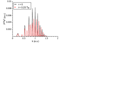
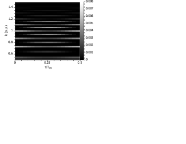
Figure 1: Photoelectron spectrum of the hydrogen atom in the polarization axis direction. Left: the probability density $P^{(3)}k^{2}$ as a function of the photoelectron momentum $k$ for two fixed values of $\tau$. Right: a gray scale map of $P^{(3)}(k,\tau)k^{2}$.

This characteristic behavior is clearly seen in Fig. 1 where we display the photoelectron spectrum of the hydrogen atom subjected to an APT with the central frequency $\omega_{\rm XUV}=17\omega$. Here and in examples below, we set $\omega_{\rm XUV}$ such that the ”central” peak in the photoelectron spectrum is positioned at $E_{2q_{0}+1}\approx 0.5$ a.u. We set the photoelectron detection angle to $\theta=0$ which corresponds to the polarization axis direction. By the least square fit to Eq. (37), we obtained the values of $\tau_{a}$ shown in Fig. 2. Here the atomic time delay is exhibited as a function of the photoelectron energy $E_{e}=k^{2}/2$. The corresponding sideband indices are marked in the figure. To test the numerical stability of our computational procedure, we performed three sets of calculations: a) the radial grid step $\Delta\xi=0.2$ and the number of spherical harmonics $N_{\theta}=4$; b) $\Delta\xi=0.1$ and $N_{\theta}=4$; c) $\Delta\xi=0.2$ and $N_{\theta}=8$. It is clearly seen from Fig. 3 that an increase of the angular basis size $N_{\theta}$ does not affect the result. For lower photoelectron energy, the time delay is not sensitive to the radial grid step. However, such a sensitivity becomes noticeable for higher photoelectron energy $E_{e}>25$ eV.

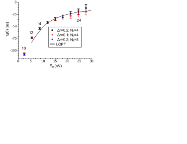
Figure 2: Atomic time delay $\tau_{a}$ of the hydrogen atom in the polarization axis direction as a function of the photoelectron energy $E_{e}$. Radial and angular numerical parameters are displayed in the legend. Error bars indicate the least squire fit uncertainty. The solid line visualizes the LOPT result of Dahlström et al. (2012). Sideband indices made on the figure correspond to the four panels of Fig. 3.

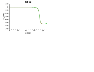
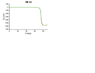
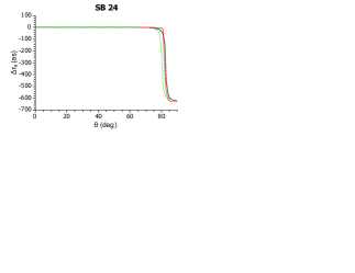
Figure 3: Angular-dependent part of the atomic time delay $\Delta\tau_{a}=\tau_{a}(E_{e},\theta)-\tau_{a}(E_{e},0)$ for the hydrogen atom as a function of the photoelectron emission angle $\theta$ relative to the polarization axis. The four panels correspond to different sideband indices. Different line styles visualize three sets of radial and angular grid parameters as indicated in the legend of Fig. 2.

Same sensitivity to the radial and angular grid parameters can be seen in Fig.3 where we display the angular dependent part of the atomic time delay $\Delta\tau_{a}=\tau_{a}(E_{e},\theta)-\tau_{a}(E_{e},0)$ for the hydrogen atom as a function of the photoelectron emission angle $\theta$ relative to the polarization axis. Based on this calibration, we restricted ourselves to $\Delta\xi=0.1$ and $N_{\theta}=4$ to all the atomic calculations shown below. For the H${}_{2}^{+}$ ion, we used a larger angular basis with $N_{\theta}=16$ to account the for the non-spherical ionic potential.

Further calibration of our technique is demonstrated in Fig. 4 where we compare the atomic time delay of the helium atom at $\omega_{\rm XUV}=25\omega$ with the results of direct numerical solution of the TDSE in the SAE Heuser et al. (2016). In both sets of the TDSE calculations, the non-local potential of the He atom was modeled by an analytical parametrization Sarsa et al. (2004). Close resemblance of the two sets of data can be seen.

We note in passing that the numerical TDSE SAE results reported in Heuser et al. (2016) required many hours of supercomputer time whereas the present calculations were carried on a notebook computer in less than an hour.

Angular dependent part of the time delay in He is exhibited in Fig. 5 where we make a comparison with other calculations reported in Heuser et al. (2016). Our modeling showed that the angular-dependent part of the time delay, unlike the energy-dependent part, is sensitive to the APT width $\tau_{\rm APT}$. This is illustrated in the figure where we present the two set of calculations with $\tau_{\rm APT}=2T_{\rm IR}$ and $\tau_{\rm APT}=1.32T_{\rm IR}$ as in Heuser et al. (2016). The latter results are particularly close to both the SAE and ab initio TDSE results from Heuser et al. (2016).

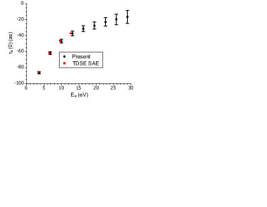
Figure 4: Atomic time delay $\tau_{a}$ of the helium atom as a function of $E_{e}$ for ejection angle $\theta=0^{\circ}$ and various sets of numerical parameters. Error bars display the uncertainty of the least square fit. The TDSE SAE results from Heuser et al. (2016) are also shown for comparison.

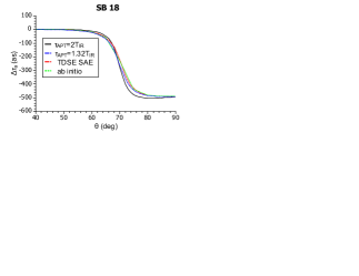
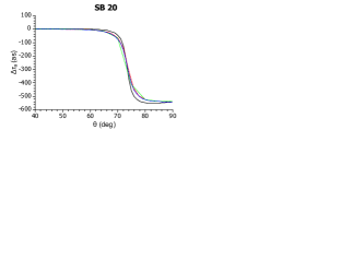
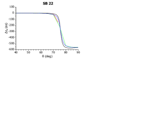
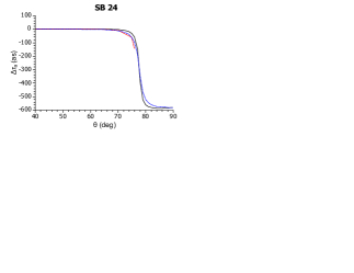
Figure 5: Angular-dependent part $\Delta\tau_{a}$ of the atomic time delay in He as function of electron ejection angle $\theta$ for four fixed SBs. The present results for $\tau_{\rm APT}=2T_{\rm IR}$ (black solid line) and for $\tau_{\rm APT}=1.32T_{\rm IR}$ (blue dash-dotted line) are shown . Also displayed are the TDSE SAE (red dashed line) and TDSE ab initio (green dotted line) results from Heuser et al. (2016).

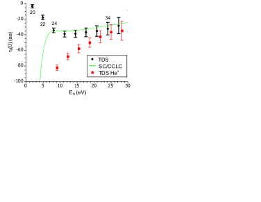
Figure 6: The time delay $\tau_{a}$ for H${}_{2}^{+}$ as a function of the photoelectron ejection energy $E_{e}$ at a fixed ejection angle $\theta=0$. The SC/CCLC results (green dotted line) and TDS results for He⁺ (red squares) are also shown for comparison. Sideband indices made on the figure correspond to the four panels of Fig. 7

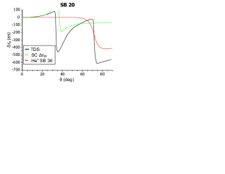
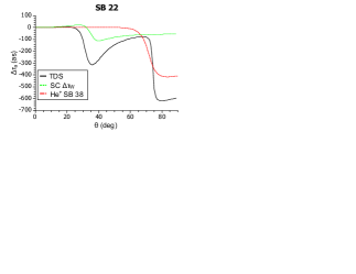
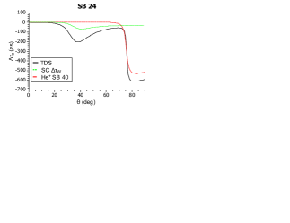
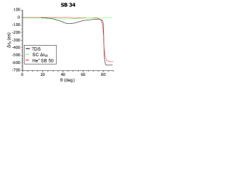
Figure 7: The angular variation of the time delay $\Delta\tau_{a}$ (black solid line) and Wigner’s time delay $\Delta\tau_{W}=\tau_{W}(E_{e},\theta)-\tau_{W}(E_{e},0)$ (green dotted line) of H${}_{2}^{+}$ for several fixed photoelectron energies $E_{e}$. The TDS results for He⁺ for SBs with close energies are also shown (red dashed line).

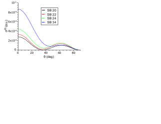
Figure 8: The triple-differential cross section $\sigma^{(3)}$ of ionization of H${}_{2}^{+}$ by monochromatic XUV as function of $\theta$ for several fixed photoelectron energies $E_{e}$ equal SB energies on Fig. 7.

Finally, we demonstrate the efficiency of our technique by original calculations of the atomic time delay in the H${}_{2}^{+}$ molecular ion. In these calculations, the central frequency of the APT was set to $\omega_{UV}=27\omega$. A polarization of the field is parallel to the molecular axis. The energy and angular variation of the time delay in H${}_{2}^{+}$ are displayed in Fig. 6 and Fig. 7, respectively. Both these dependencies are very different from that of atomic H and He. The energy variation of $\tau_{a}$ with $E_{e}$ for H${}_{2}^{+}$ is non-monotonous. The angular dependence of H${}_{2}^{+}$ displays an additional strong variation in the range of emission angles $\theta=30^{\circ}-50^{\circ}$. To visualize clearly this molecular effect, we make a comparison of the angular dependent time delay in H${}_{2}^{+}$ with the spherically symmetric He⁺ ion. To account for different ionization potentials, we carried out the He⁺ calculation at the central frequency $\omega_{\rm XUV}=43\omega$. It is clearly seen that the atomic and molecular ions display the angular dependent time delay which differs considerably not only by additional strong angular variation but also the magnitude of the sharp drop of the time delay near the $90^{\circ}$ emission angle. We note that the asymptotic field of the ion remainder is the same in both cases. Hence should be the same the CLC term of the atomic time delay (8). Therefore the difference of the atomic time delay in the H${}_{2}^{+}$ and He⁺ ions should be attributed largely to the Wigner component $\tau_{\rm W}$ of the time delay.

This component is related to the monochromatic XUV photoionization and can be expressed via the logarithmic derivative of the corresponding photoionization amplitude:

$$\tau_{\rm W}={\rm Im}\left[\frac{1}{f_{\rm XUV}(\mathbf{k})}\frac{\partial f_{\rm XUV}(\mathbf{k})}{\partial E_{e}}\right].$$ (38)

The angular differential XUV cross-section is expressed via the same amplitude as

$$\sigma^{(3)}=\frac{d^{3}\sigma}{dE_{e}d\Omega_{e}}=\frac{4\pi^{2}\omega_{\rm XUV}}{c}k|f_{\rm XUV}(\mathbf{k})|^{2}$$ (39)

By inspecting these two equations, we observe that the minimum of the angular differential XUV cross-section corresponds to the maximum of the Wigner time delay. This can be indeed confirmed by aligning Fig. 7 with Fig. 8 where we exhibited the angular differential XUV cross-section for the corresponding sidebands.

Ionization of H${}_{2}^{+}$ by a monochromatic XUV radiation was modeled separately by the method based on the spheroidal Coulomb (SC) functions Serov et al. (2002, 2005). With this method, we obtained the XUV ionization amplitude and fed it to the expression for the Wigner time delay Eq. (38) and differential cross-section (39). The Wigner time delay was also estimated by a classical approximation to CLC (CCLC) derived in Serov et al. (2015) for the case of $\theta=0$:

$$\tau_{a}\approx\frac{\tau_{\rm W}+[a\ln(k/Z)+I_{c}(a)]/\omega}{1-I_{s}(a)}$$ (40)

with the parameter $a=Z\omega/k^{3}$ and functions

$$I_{c}(a) = -a[\ln(2/a)-1-\gamma]-\frac{3\pi}{4}a^{2};$$

$$I_{s}(a) = -\frac{\pi}{2}a+\frac{3}{2}a^{2}[\ln(2/a)-1/6-\gamma]$$

Here $\gamma=0.577$ is the Euler constant. It is seen in Fig. 6 that for $E_{e}>8$ eV results of SC/CCLC are rather close to those obtained from our TDS RABBITT simulations. However, at lower energies, SC/CCLC fails. One can observe in Fig. 7 that the angular variation of the Wigner time delay is qualitatively similar to variation of $\tau_{a}$, but a quantitative difference is quite noticeable. This means that the CLC correction $\tau_{\rm CLC}$ is not a universal function that fits Eq. (8) both for the He⁺ and H${}_{2}^{+}$ ions.

The interference character of the minimum in the angular differential cross-section is revealed by its shift to the right when the photon and photoelectron energy increase. An additional minimum appears at small angles when the photoelectron energy exceeds 200 eV but this energy range is not visualized in the figure. The relative depth of the minimum of the angular differential cross-section increases closer to the threshold. Accordingly, the magnitude of the oscillation of the Wigner time delay and the atomic time delay grows bigger in lower side bands. As it was demonstrated in Serov et al. (2013), this the deepening of the minima is related to appearance of a near threshold Cooper minimum. This minimum has an angular character as the dipole component of the ionization amplitude vanishes giving way to a octupole component.

IV Conclusion

We have developed an efficient computational technique for solving the time-dependent Schrödinger equation. As an illustration, we applied this scheme to the process of two-color XUV/IR photoionization of the molecular H${}_{2}^{+}$ ion. Up to now, this process could only be described by a simplified 2D model Chelkowski and Bandrauk (2010). We derived the energy and angular dependent photoemission time delay and connected its peculiarities with the photoelectron group delay (Wigner time delay) and the Coulomb-laser coupling induced correction. The Wigner time delay carries a strong imprint of the interference structure in the angular resolved XUV photoionization cross-section. The Coulomb-laser coupling correction is similar in the atomic He⁺ and molecular H${}_{2}^{+}$ ions and is determined largely by the asymptotic part of the photoelectron wave packet propagating in the Coulomb field of the ion remainder and the dressing IR field.

As a further development, we will expand our technique to describe the photoemission time delay in H₂ and other diatomic molecules. Experimental observation of time delay in such systems has now become possible Vos et al. (2016).