Regularizing Solutions to the MEG Inverse Problem Using Space–Time Separable Covariance Functions
Abstract
In magnetoencephalography (MEG) the conventional approach to source reconstruction is to solve the underdetermined inverse problem independently over time and space. Here we present how the conventional approach can be extended by regularizing the solution in space and time by a Gaussian process (Gaussian random field) model. Assuming a separable covariance function in space and time, the computational complexity of the proposed model becomes (without any further assumptions or restrictions) , where is the number of time steps, is the number of sources, and is the number of sensors. We apply the method to both simulated and empirical data, and demonstrate the efficiency and generality of our Bayesian source reconstruction approach which subsumes various classical approaches in the literature.
1 Introduction
Magnetoencephalography (MEG) is a non-invasive electrophysiological recording technique that is widely used in the neuroscience community (Cohen, 1972). It provides data at high temporal resolution and the signal measured at each MEG sensor provides an instantaneous mixture of active neuronal sources.
Reconstruction of neuronal source time-series from sensor-level time-series requires the inversion of a generative model. This inverse problem is fundamentally ill-posed and additional assumptions with respect to the parameters of the neuronal sources are required. Two types of generative models have been proposed for neuromagnetic inverse problems: equivalent current dipole models and distributed source models (see, e.g., Baillet et al., 2001). Equivalent current dipole models can be estimated via Bayesian particle filtering methods (see, e.g., Sorrentino et al., 2009; Chen et al., 2015, and the references therein). In the following, we focus on the distributed source models, which assume an extensive set of predefined source locations associated with unknown current amplitudes.
Over the past decades, various distributed inverse modelling techniques have been proposed and applied to neuroscience data, all of which impose their own assumptions. Commonly used techniques include the minimum-norm estimate (MNE) (Hämäläinen & Ilmoniemi, 1994) and the minimum-current estimate (Uutela et al., 1999), which both penalize source currents with large amplitudes but where the latter produces more sparse estimates, the low resolution electromagnetic tomography (LORETA) (Pascual-Marqui et al., 1994), which promotes spatially smooth solutions, as well as different spatial scanning and beamforming techniques (van Veen et al., 1997; Mosher & Leahy, 1998). Various extensions and modifications of these methods have been published including depth-bias compensations and standardized estimates (Fuchs et al., 1999; Dale et al., 2000; Pascual-Marqui, 2002) and Bayesian frameworks for source and hyperparameter inference as well as model selection (Trujillo-Barreto et al., 2004; Serinaĝaoĝlu et al., 2005).
To improve localization accuracy, various different spatial priors have been proposed including spatially informed basis-functions whose parameters are learned from data in a Bayesian manner (Phillips et al., 2005; Mattout et al., 2006), and smoothness-promoting spherical harmonic and spline basis functions (Petrov, 2012) as well as various sparsity-promoting priors (Gorodnitsky et al., 1995; Sato et al., 2004; Auranen et al., 2005; Nummenmaa et al., 2007; Haufe et al., 2008; Wipf & Nagarajan, 2009; Wipf et al., 2010; Lucka et al., 2012; Babadi et al., 2014). Other approaches to improve the localization accuracy include combined models for simultaneous noise suppression (Zumer et al., 2007), and models for potential inaccuracies in the forward model (Stahlhut et al., 2011).
Most of the previously mentioned distributed source reconstruction techniques assume temporal independence between the source amplitudes, which does not make use of all the available prior information on the temporal characteristics of the neuronal currents. For this reason, many spatio-temporal techniques have been proposed including models based on different spatio-temporal basis functions and carefully designed or empirically learned Gaussian spatio-temporal priors (Baillet & Garnero, 1997; Darvas et al., 2001; Greensite, 2003; Daunizeau et al., 2006; Friston et al., 2008; Litvak & Friston, 2008; Trujillo-Barreto et al., 2008; Bolstad et al., 2009; Limpiti et al., 2009; Dannhauer et al., 2013). Many approaches are specifically targeted to obtain spatially sparse but temporally informed, smooth or oscillatory source estimates (Cotter et al., 2005; Valdés-Sosa et al., 2009; Ou et al., 2009; Haufe et al., 2011; Zhang & Rao, 2011; Tian et al., 2012; Gramfort et al., 2012, 2013; Lina et al., 2014; Castaño-Candamil et al., 2015). Dynamic extensions have been proposed also for spatially decoupled beamforming techniques (Bahramisharif et al., 2012; Woolrich et al., 2013).
Dynamical state-space models are a very intuitive way of defining spatio-temporal source priors. Many of the proposed approaches typically assume a parametric spatial structure derived from spatial proximity or anatomical connectivity, and a low-order multivariate autoregressive model for the temporal dynamics (Yamashita et al., 2004; Galka et al., 2004; Long et al., 2011; Lamus et al., 2012; Pirondini et al., 2012; Liu et al., 2015; Fukushima et al., 2015). FMRI-informed spatial priors have also been proposed in (Daunizeau et al., 2007; Ou et al., 2010; Henson et al., 2010). Another class of spatio-temporal priors assumes that the sparsity is encoded in the the source scales rather than amplitudes, which is the key assumption used by the multivariate Laplace prior (van Gerven et al., 2009) as well as the structured spatio-temporal spike-and-slab priors (Andersen et al., 2014, 2015).
In the present work, we show that high-quality Bayesian inverse solutions that employ various forms of spatio-temporal regularization can be obtained in an efficient manner by employing Gaussian processes (GPs) that use space–time separable covariance functions. These models are also referred to as Gaussian random fields. As infinite parametric models, GPs form a flexible class of priors for functions (see, e.g., Rasmussen & Williams, 2006) and they have been successfully applied in various inverse problems (see, e.g., Tarantola, 2004). They are particularly suitable for spatio-temporal regularization because stationary GPs can also be interpreted as linear stochastic dynamical systems with a Gaussian state-space representation, which is the typical way of modelling physical systems (Särkkä et al., 2013). The inference can be done either using batch solutions or Kalman filtering and smoothing, and different GP priors can be easily combined to form, for example, temporally smooth and/or oscillatory sources with spatially smooth structure.
Our approach is most closely related to previous approaches based on spatio-temporal basis functions or empirically informed prior covariance structures proposed by Darvas et al. (2001); Greensite (2003); Friston et al. (2008); Trujillo-Barreto et al. (2008); Bolstad et al. (2009); Limpiti et al. (2009); Dannhauer et al. (2013). A key difference is that a finite set of basis functions is replaced by an infinite-dimensional process, or a combination of additive processes. The spatio-temporal characteristics of the resulting prior can be tuned by adapting covariance function hyperparameters in a data-driven empirical Bayesian manner (Rasmussen & Williams, 2006).
Using both simulation studies and empirical data (Kauramäki et al., 2012), we show that our approach is able to recover source estimates at a high degree of accuracy. Moreover, we show that various existing source reconstruction approaches (e.g., Hämäläinen & Ilmoniemi, 1994; Petrov, 2012) are special cases of our framework that use particular spatial covariance functions. Various methodological developments ensure that our approach scales well with the number of sources and sensors. Furthermore, since the framework implements a Bayesian approach we also gain access to uncertainty estimates about the location of the recovered sources, and we can determine maximum posteriori estimates of the model hyperparameters in a principled manner.
Summarizing, as demonstrated on simulated as well as empirical data, the generality and efficiency of our framework open up new avenues in solving MEG inverse problems.
2 Methods and Materials
2.1 MEG forward problem
In magnetoencephalography (MEG) the biomagnetic fields produced by weak currents flowing in neurons are measured non-invasively with multichannel gradio- and magnetometer systems. For reviews on MEG methodology see, for example, Hämäläinen et al. (1993) and Baillet et al. (2001). For now, we disregard any further information on how the model is described and derived using physical constraints, and we only consider a general-form linear forward model. Standard references on the mathematical model for MEG are Sarvas (1987) and Geselowitz (1970).
Following the notation of Sarvas (1987), we consider a forward model with a number of sources (size of the brain mesh) and sensors. Let the forward model with a number of sources and sensors be
| (1) |
where indexes time, is the lead-field matrix, are the sensor readings, and the source values. The observations are corrupted by a noise term, that is assumed Gaussian, . We assume the noise covariance matrix to be known, that is, not part of the estimation procedure.
As usual, only the quasi-static forward problem is considered in this context, and if we assume the forward problem to be time-invariant, we can rewrite the forward model for the entire range of observations in time. Let , , and be the values at time instant . This model can still be formulated by stacking the values into columns, such that
| (2) |
where corresponds to the sensor reading columns, and to the column-wise source values. The noise term consists of columns, , for . Equivalently we can write the observation model (2) in a vectorized form as
| (3) |
where . Operator denotes the vectorization of matrix , which is obtained by stacking the columns of on top of one another and results in a column vector, and denotes the Kronecker product, which is obtained by stacking together submatrices vertically for and horizontally for (see, e.g., Horn & Johnson, 2012).
Without loss of generality, we consider a model that has been whitened by the eigenvalue decomposition of the noise covariance matrix: , where we retain only the positive eigenvalues. Multiplying (2) from the left by gives a whitened model such that , , and . For the remainder of the paper we will assume that the model is whitened and drop the tildes to simplify the notation.
It is possible to extend the proposed approach to include an estimate of the temporal structure of the noise in the form of a covariance matrix . In this case we write the noise covariance of the vectorized model (3) as a Kronecker product of a spatial and a temporal covariance matrix, that is, . Computing the eigendecomposition and multiplying the vectorized model (3) from the right by , results in a whitened model , where . All the subsequent results can be derived using this modified model with the main requirement being that the observation matrix is of spatio-temporal Kronecker form.
2.2 Gaussian process based regularization in space and time
Our interest is in the inverse problem of finding the state of the sources given the sensor readings. The number of sources (typically in thousands) is much larger than the number of sensors (typically some hundreds), making the inverse problem underdetermined. Thus, in general, its solution is non-unique. Therefore we will regularize the solution by injecting prior knowledge concerning properties of the unknown underlying state of the neuronal generators of the MEG signal in the cerebral cortex.
We employ Gaussian process (GP) priors in order to regularize the solution of the inverse problem in space and time. In this section we first give the general form of the method, and then we show how the problem can be reformulated under the assumption of separable covariance functions. Separability in this context means the covariance structure factors into a purely spatial and purely temporal component. This does not restrain the model from coupling spatial and temporal effects in source-space, but restrains the model from enforcing coupling between arbitrary spatial and temporal locations explicitly.
The prior assumptions of the latent neuronal behavior on the cortex are encoded by a Gaussian process prior (Gaussian random field), which has structure both in space and time. We define the Gaussian process (see, e.g., Rasmussen & Williams, 2006; Tarantola, 2004) as follows.
Definition 2.1 (Gaussian process).
The process , is a Gaussian process on with a mean function , and a covariance function (kernel) , if any finite collection of function values has a joint multivariate Gaussian distribution such that , where and , for .
Consider the inputs consisting of both the spatial and temporal points on the cerebral cortex, . We assign the following zero-mean Gaussian process prior (without loss of generality)
| (4) |
such that and assume that the observations are given by the forward model as defined in the previous section:
| (5) |
We can interpret the problem as a Gaussian linear model, with a marginal Gaussian distribution for and a conditional Gaussian distribution for given of the form
where the elements of the prior covariance matrix are given by .
Following the above model, we can analytically compute the posterior distribution of by conditioning on . Under the functional space view of the GP regression problem, we consider an infinite set of possible function values and predict for any by integrating over and conditioning on . The solution to the Gaussian process regression prediction problem can be given as follows. Consider an unknown latent source reading at . Conditioning on the observations gives predictions , where the mean and variance are given by
| (6) | ||||
| (7) |
where is an -dimensional vector with the :th entry being and is an matrix. This result is readily available. These equations are derived, for example, in (Bishop, 2006, p. 93).
2.3 Spatio-temporal regularization of space-time separable GPs
For implementing Equations (6) and (7), the dimensionality of the problem becomes an issue. For example, consider an MEG dataset of moderate size with and observations. This means that the matrix to invert would be of size , which renders its practical use largely impossible.
To circumvent this problem, in the following, we assume that the covariance structure of the underlying GP is separable in space and time. In the prewhitening step, we required also similar separability for the noise covariance. The following separable structure of is assumed:
| (8) |
meaning that the kernel is separable in space and time. The covariance matrix corresponding to this covariance function is thus
| (9) |
where the temporal and spatial covariance matrices are defined as , for , and , for . We write down the eigendecompositions of the following covariance matrices: and . We denote the eigenvalues of the matrices and . This brings us to the key theorem of this paper, a proof of which can be found in A.
Theorem 2.2 (Spatio-temporal regularization).
Consider an unknown latent source reading in a source mesh point at an arbitrary time-instance . Conditioning on all the observations and integrating over gives a predictive distribution
| (10) |
where the mean and variance are given by
| (11) | ||||
| (12) |
where is an -dimensional vector with the th entry being , is an -dimensional vector with the th entry being , and is the matrix of measurements. The matrix has elements , and by ‘’ we denote the Hadamard (element-wise) product.
Compared to traditional point-estimate based inverse solutions, Theorem 2.2 offers a flexible and computationally efficient Bayesian alternative, which enables principled probabilistic posterior summaries of the sources, efficient gradient-based estimation of regularization hyperparametes, and implementation of various existing regularizers as described in the following sections.
2.4 Quantifying uncertainty about source estimates
Probabilistic posterior summaries can be computed using the Gaussian marginal posterior (10) for any chosen time instant and source location. For example, instead of summarizing only the mean , where , we can compute the marginal posterior probability for the source activation to be positive as , where is the Gaussian cumulative distribution function. This probability equals one if all the marginal probability density is located strictly at the positive real axis and zero in the opposite case.
2.5 Encoding prior beliefs with covariance functions
Within the GP framework, prior beliefs on source activations in space and time are encoded via different choices of kernels (covariance functions). In this section, we explore a number of alternative separable kernels functions of the form . We first consider spatial kernels and assume temporal independence such that the temporal kernel is defined as , where if and zero otherwise. We will show that some of these spatial kernels correspond to (Bayesian variants of) source reconstruction algorithms that are used in the literature. After considering spatial kernels, we will consider an example of a spatio-temporal kernel in which we drop the temporal independence assumption.
2.5.1 Minimum norm estimation
If, next to temporal independence, we assume spatial independence, we obtain a covariance function that corresponds to a minimum norm estimate (MNE) solution (Hämäläinen & Ilmoniemi, 1994). This covariance function makes use of the kernel:
| (13) |
where is a magnitude parameter that controls the prior variance of the source current amplitudes. Coupled with the temporal independence assumption, this kernel results in diagonal covariance matrices and .
Remark 2.3.
This shows that the presented framework can be used to compute a Bayesian equivalent of the MNE estimate. In contrast to the traditional view, the Bayesian version offers also probabilistic uncertainty estimates of the source amplitudes via (12) as well as a convenient proxy for determining the regularization parameter from the observed data using the marginal likelihood as described in Section 2.6.
2.5.2 Exponential covariance function
As Gaussian processes are formulated as non-parametric models, covariance functions can be interpreted as spanning the solution with an infinite number of possible basis functions. A canonical example is the exponential covariance function which is given by the kernel
| (15) |
where is a magnitude hyperparameter and is the characteristic length scale. Exponential covariance functions encode an assumption of continuous but not necessarily differentiable sample trajectories. In one dimension such processes are also known as Ornstein–Uhlenbeck processes (see, e.g., Rasmussen & Williams, 2006).
2.5.3 Matérn covariance function
An alternative to the exponential covariance function is the Matérn covariance function (with smoothness parameter ), which is given by the kernel
| (16) |
This kernel produces estimates which are more smooth than those produced by an exponential prior. In the one-dimensional case, the Matérn covariance function encodes the assumption that the sample trajectories are continuous once-differentiable functions.
2.5.4 Gaussian covariance function
Another often used formulation is given by the Gaussian covariance function, which uses the radial basis function (RBF) kernel
| (17) |
This kernel encodes the assumption of infinitely smooth (infinitely differentiable) processes.
2.5.5 Harmony covariance function
The exponential, Matérn and Gaussian kernels are examples of nondegenerate kernels that have an infinite number of eigenfunctions (Rasmussen & Williams, 2006). We can alternatively make use of degenerate kernels that can be described in terms of a finite number of eigenfunctions.
We here consider a model which assumes that the inference is done on a spherical surface and which has been considered in the literature before. The Harmony (HRM) model by Petrov (2012) is based on a projection of the inference problem onto spherical harmonical functions. Higher frequencies are suppressed in this approach by down-weighting them (Petrov, 2012). Recalling that Cartesian coordinates on the spherical hull correspond to in spherical coordinates, the Harmony model can be re-written as a weighted set of standard spherical harmonic basis functions
| (18) |
where is the total number of spherical harmonic basis functions (terms in the sums), denotes the harmonic index, is the magnitude hyperparameter, and a spectral weight (length-scale) hyperparameter. The fraction term defines the spectrum of the model. The Laplace’s spherical harmonic functions are defined as (see, e.g., Arfken & Weber, 2001):
| (19) |
where denotes the associated Legendre polynomials. Spherical harmonics are smooth and defined over the entire sphere. They can thus induce spurious correlations if too few basis functions are included in the model, or the weighting of the higher-frequency components is inconsistent. However, they span a complete orthonormal basis for the solution. Petrov (2012) used harmonic basis functions and chose by minimizing a measure on the localization error in a set of simulated inverse problems.
2.5.6 Spline covariance function
To avoid spurious correlations in the Harmony model, one option is to make the basis functions local. The spline (SPL) model by Petrov (2012) considers evenly spaced splines on the spherical hull, whose weighted superposition gives the following kernel:
| (20) |
Here denotes the Abel–Poisson kernel centered at , which is given by Freeden & Schreiner (1995):
| (21) |
where is a length-scale hyperparameter. Following Petrov (2012), we use spherical splines uniformly positioned on both cortical surfaces with located at the nodes of the second subdivision of icosahedron meshing. The SPL model captures small-scale phenomena well, but is somewhat sensitive to where the splines are placed.
Increasing the number of splines diminishes the effect of the spline placement related artefacts. Using the connection between the Poisson kernel in multipole expansions and the Cauchy distribution, there is a relationship between this spline kernel and a more general class of covariance functions. If the number of splines , this degenerate kernel approaches the following nondegenerate kernel (up to a scaling factor):
| (22) |
where the decay parameter . This is known as the rational quadratic (RQ) covariance function (see Rasmussen & Williams, 2006, for a similar parametrization). By this connection, we may recover the characteristic length-scale relation between the spline kernel and the family of nondegenerate kernels we have presented. Petrov (2012) set the spline scale parameter to by minimizing a measure on the localization error in a set of simulated inverse problems. This corresponds to a characteristic length-scale of .
2.5.7 Spatio-temporal covariance function
So far, we assumed temporal independence. However, next to using different formulations for the spatial kernel, we can also use different formulations for the temporal kernel that drop the temporal independence assumption. Here, we only consider one such formulation of a spatio-temporal kernel that is written in terms of spatial and temporal exponential kernels:
| (23) |
Because the exponential kernel presumes continuity but not necessarily differentiability, we regard it as a good general purpose kernel for settings where there is no exact information about the smoothness properties of underlying source activations. However, it should be stressed that we use the exponential spatio-temporal kernel mainly for the purpose of illustration as the generality of our framework allows for arbitrary choices of spatial and temporal kernels.
2.6 Hyperparameter optimization
The hyperparameters of the covariance function were earlier suppressed in the notation for brevity. In a typical spatio-temporal GP prior setting following (23) the hyperparameter vector consists of the magnitude parameter and the spatial and temporal length-scales: . For finding the hyperparameters, we consider the marginal likelihood of the model. The negative log marginal likelihood for the spatio-temporal model is
| (24) |
The eigenvectors and the eigenvalues depend on the hyperparameters , and in general re-calculating the eigendecompositions are required if the parameters change. However, for the magnitude parameter this is not required, as it can be seen as a scaling factor of the prior covariance . This means that if the length-scales are fixed, the eigendecompositions need to be computed only once, and during the subsequent optimization can be added as a multiplier to either all s or all s. Similarly, if either of the length-scale variables is fixed, the corresponding eigendecomposition does not need to be recomputed.
2.6.1 Choosing the spatial and temporal length-scales
The strongly ill-posed inverse problem and the potentially multimodal marginal likelihood make a purely data-driven estimation of the hyperparameters challenging. In parametric models, the scale of the modeled phenomena is often tuned by choosing an appropriate number of basis functions. Under the non-parametric setting, however, the characteristic length-scale hyperparameter tunes scale-variability of the estimate.
One option to facilitate the hyperparameter estimation is to inject prior information into the model by using an informative prior and determine the maximum a posteriori estimate of . A prior to the temporal length-scale could be chosen so that the spectral bandwidth of the source amplitudes is at some reasonable region. For example, in the empirical experiments we chose a fixed value for the temporal length-scale, ms, which enables the model to explain well the most quickly-varying peaks of the averaged event-related potentials. The solution is not sensitive to the choice of the temporal length-scale, because optimizing the magnitude parameter compensates for small changes in . This can be verified by comparing the predictive distribution of the sensor reading with the observed data.
A prior for the spatial length-scale can be chosen by acknowledging the natural spatial cutoff frequency that arises from the finite number of MEG channels by the Nyquist limit. For and a distance measure defined on the unit sphere, this corresponds to a minimal spatial length-scale of in the case of an exponential kernel. Another viable approach to choose the spatial length-scale could be to simulate various kinds of source activation patterns and choose the spatial length-scale value that maximizes the localization accuracy in terms of some suitable measure as proposed by Petrov (2012). As presented in the previous sections, the chosen parameters in Petrov (2012) correspond to a characteristic length-scale of roughly , while the low-rank nature of Harmony favors large-scale smooth activations.
To avoid making too strong spatial smoothness assumptions, we fixed the spatial length-scale to in the empirical comparisons. This compensates for the non-ideal distance measures, which are not truly isotropic but given along the spherical cortex model. Optimizing the magnitude parameter with fixed temporal and spatial length-scales allows the model to explain the observed data well and compensates for small uncertainty regarding this choice of fixed length-scales.
2.7 Computational complexity
The most critical computations for evaluating the predictions (11) and (12), as well as the marginal likelihood (24), are the eigendecompositions and , which scale as and respectively. The savings are significant compared with the naive implementation of (6) and (7) which scales as . The eigendecompositions need to be recomputed only once after adjusting the covariance function hyperparameters that control and . For fixed prior covariances, the decompositions need to be computed only once.
In practice, the decomposition of is insignificant because typically . The decomposition of can become problematic if grows too large but for typical MEG studies with up to few thousand time points per trial the inverse analysis can be done in few seconds using a standard PC. With small to mediocre , the additional cost for spatio-temporal GP inverse analysis is negligible compared to the standard MNE estimate.
2.8 Simulated data
In order to compare the behaviour of the various introduced priors in the spatial dimension, we made use of simulated data. Data were simulated by simultaneously activating two distinctive source patches. The sources were located on opposite cerebral hemispheres, and together they measured roughly 9.2 cm2 in size (measured along the cortical surface). Dipole orientations were fixed to be orthogonal to the cortical surface. The strength of the source dipoles was chosen such that they replicated the sensor data from the experimental recordings ( Volts), and Gaussian noise with a covariance structure from a pre-measurement empty-room batch of data was added to the simulated data sets. Typical running times for our simulations using independent, spatial, temporal and (separable) spatio-temporal priors are summarized in Table 1.
| Method | Mean running time [s] | Max running time [s] |
|---|---|---|
| MNE (independent) | 13.26 | 17.44 |
| GP (spatial) | 25.37 | 32.26 |
| GP (temporal) | 30.97 | 35.87 |
| GP (spatio-temporal) | 42.11 | 51.67 |
2.9 Empirical data
In order to empirically validate our approach we made use of the data described in Kauramäki et al. (2012). The goal of this study was to further our understanding of selective attention to task-relevant sounds whilst ignoring background noise. In the present paper, we use a subset of the data in order to study source reconstruction results under different GP regularisation schemes. We briefly describe the main characteristics of these data.
A subset of 10 subjects (7 males) out of 14 subjects was used in our analyses as their cortical surface reconstructions from whole-head anatomical MRI images were readily available. All subjects signed a written informed consent before the study. The measurements conformed to the guidelines of the Declaration of Helsinki, and the research was approved by the ethical committee in the Hospital District of Helsinki and Uusimaa. The task of the subjects was to attend either to the auditory or visual stream, and to respond by lifting a finger whenever an attended target stimulus occurred. The task was alternated every two minutes with instructions on screen, with two auditory and two visual tasks in each 8-minute block. This was repeated eight times with short breaks in between.
In this study we consider the auditory condition only. Subjects were presented with 300 ms tones of 1000 Hz (‘standard’, 90% of sounds) and 1020 Hz (‘target’, 10% of sounds) frequencies. The mean interstimulus interval from onset to onset was 2 seconds (range 1800–2200 ms). The tones were played either on their own (‘no masker’ condition) or with a masker sound (7 different maskers). The continuous masker sounds (16-bit, 48-kHz) were created by filtering in the frequency domain 10-minute Gaussian white noise with symmetrical stopbands or notches around 1000 Hz. Seven different notch widths were used in order to manipulate the impact of masking (500 Hz, 300 Hz, 200 Hz, 150 Hz, 100 Hz, 50 Hz, 0 Hz). As the perceptual SNR was adjusted so that the sounds were played at individual hearing threshold, this notch width manipulation resulted in clearly poorer performance in the task with narrower notches. That is, both standard and deviant tones were harder to detect from the background noise masker. Each experimental block was run with the same continuous masker sound with the blocks jointly spanning all used notches and the no-masker background sound.
Magnetoencephalography (MEG) data was acquired using a 306-channel whole-head neuromagnetometer (Vectorview, Elekta Neuromag Oy, Helsinki, Finland). MEG data were recorded at 2000 Hz. To detect eye blinks and movements, one electro-oculogram (EOG) channel was recorded with the electrodes placed below and on the outer canthus of the left eye. Auditory-evoked responses to both standard and deviant tones were averaged. In the data analysis, whitened averaged 100–800 ms time-locked epochs were used. Epochs whose amplitudes exceeded predefined thresholds were excluded from further analysis. A prestimulus baseline of 200 ms was used to remove DC offset, and a 40 Hz lowpass filter was used during averaging. Three-dimensional locations of left and right preauricular points and nasion, four head-position indicator (HPI) coils, and a number of extra points from the scalp were used for estimating head position and alignment with cortical surface reconstruction obtained using FreeSurfer (v4.5.0, http://surfer.nmr.mgh.harvard.edu) software. A spherical head model was used to compute the lead-field matrix (Hämäläinen et al., 1993).
Kauramäki et al. (2012) showed that selective attention to sounds increased the M100 response amplitude and at the same time enhanced the sustained response. It also showed that M100 response peak amplitudes increased and latencies shortened with increasing notch width. The latter result will be used to compare source reconstruction approaches in the present study.
3 Results
In order to test our spatio-temporal GP framework for solving the MEG inverse problem, we compare how well the introduced kernels are able to recover sources of interest. To this end we make use of both simulations and empirical data.
3.1 Simulation study
We here test how the choice of spatial prior affects the spatial correlation structure of the reconstructed source configuration (assuming temporal independence). This prior information is controlled by the choice of spatial covariance function. As presented in the previous sections, the highly non-isotropic nature of the cerebral cortex can be warped through a non-linear coordinate transformation. We used a spherical inflation of the cerebral cortex for mapping the source distances.
We compared the following spatial covariance structures: MNE (spatially independent prior), the exponential covariance function, the Matérn covariance function, and the squared-exponential covariance function. For all methods, the regularization scale (magnitude) parameter was optimized by maximizing the marginal likelihood. The length-scales for HRM and SPL were chosen following the suggestions of Petrov (2012), and the length-scale of the GP covariances was chosen so that it approximately matches the decrease-rate of the spectral density of HRM covariance. Figure 1 shows the ground truth and reconstructions of the source estimates using various covariance structures in the GP reconstruction. The reconstructed sources were thresholded such that the strongest of all sources are shown for each method. This puts the different GP prior covariance functions on the same line.
Results show that all of the chosen spatial priors lead to reasonable results, in the sense that the ground truth sources are properly localised. At the same time results show that the spatially independent MNE solution yields a non-smooth result where the sign of the reconstructed source tends to fluctuate quite randomly. In contrast, the spatial GP-regularised solutions are spatially smooth showing just a few other sources with spurious activation.
Since we developed a Bayesian framework, we can also quantify the uncertainty concerning estimates of the source activations. Figure 2 shows the probability that source being positive, computed using the Gaussian marginal posterior (10). Simulations show that taking into account the predictive uncertainty by summarizing , can convey quite a different message compared to visualizing only the mean .
Given the strong correspondences between different spatially regularised priors, we restrict ourselves to the exponential covariance function in the following. In order to develop an intuition about the influence of the spatial and temporal length scale parameters for the spatio-temporal covariance function (23), Figure 3 quantifies the uncertainty when varying the length scales.
3.2 Empirical validation
In order to empirically validate our approach, as described before, we make use of the data from (Kauramäki et al., 2012). Our aim is to demonstrate the effect of GP regularization when solving the MEG inverse problem.
We consider a spatially and temporally independent baseline (MNE), a purely temporal model (spatially independent), a purely spatial model (temporally independent), and a spatio-temporal model. We used the exponential covariance function both for the temporal and spatial model. We fixed the spatial length-scale parameter to (recall that we use distances on a unit sphere) and the temporal length scale to ms. For each method, subject, and condition we optimized the magnitude hyperparameter independently by minimising the negative log marginal likelihood.
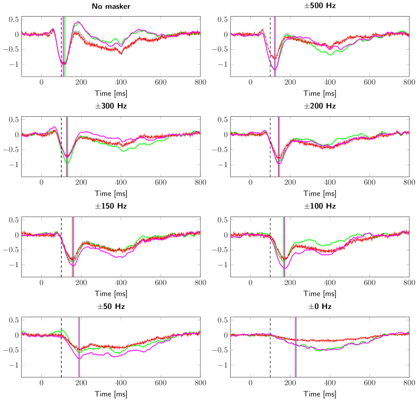
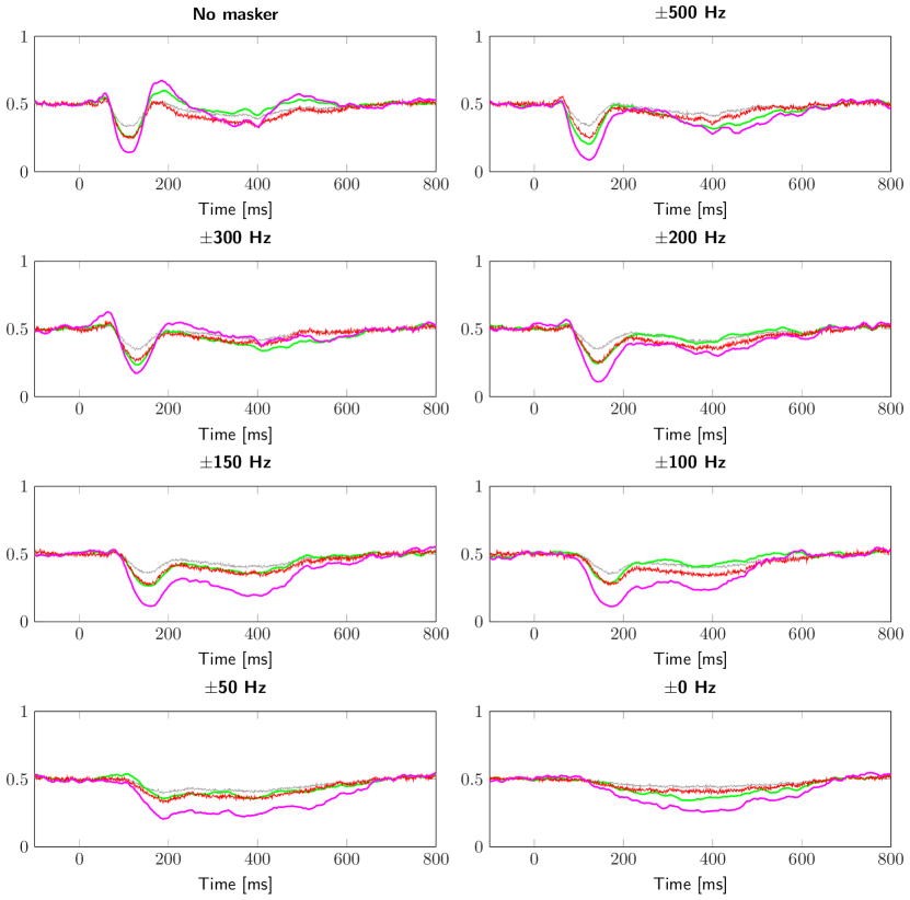
We study what the source-level ERPs look like when we attend normal vs. deviant stimuli in the auditory condition. Figure 4 shows the results for response suppression due to masking. Results for the four different methods have been scaled by their M100 peak strength under the ‘No masker’ condition. The time-series is shown for the source with the strongest contribution on the right hemisphere. We observe a gradual suppression of response amplitudes and increase in latency with narrower notches. Slightly different source waveforms are obtained for the different models. Importantly, the spatial and spatio-temporal models show more pronounced enhancement of the sustained response compared to the independent and temporal models. Figure 5 shows the corresponding posterior estimates of observing non-zero source amplitudes. The spatio-temporal model clearly shows the most marked deviations.
The probabilistic posterior summaries of the spatial structure of the activation at the estimated M100 peak corresponding to Figure 4 can be seen in Figure 6.
4 Discussion
Here, we compared traditional MNE and a number of spatial covariance selection methods from literature to our spatio-temporal GP framework; specifically how these affect the spread and reliability of the inverse solution. We show that our method is especially good in enhancing weak responses with low SNR, by comparing the results of MNE to regularized solutions with an empirical dataset where SNR was gradually reduced (Kauramäki et al., 2012). The regularized solutions retain the basic results of peak latency and amplitude modulations (Figures 4 and 7) compared to the solution obtained using traditional MNE. Further, these solutions reliably place the activity estimate at a neuroanatomically plausible location, even at low-SNR conditions (Fig. 6) where MNE estimates have much more uncertainty in auditory areas. The GP-regularized solutions yield spatially smooth estimates, as shown in Figure 1, and can reliably separate distinct sources with low uncertainty.
The spatio-temporally regularized inverse solution offers a wealth of applications for neuroscience studies employing MEG, where the interests are towards experiments using more complex, continuously changing natural stimuli, and mapping spatiotemporal specificity of brain areas with ever-higher resolution. One potential benefit of this method is in tracking fast dynamic changes of cortical activity in humans, where EEG and MEG still excel over alternative methods (Hari & Parkkonen, 2015). Increasing the robustness of inverse solutions can ultimately reduce the number of trials required to obtain a reasonable-SNR averaged evoked response, which allows tracking of small dynamic changes of cortical reactivity during for instance top-down modulation by employing subaveraging of responses throughout the course of an experiment. Further, the possibility to use weak stimulus intensities and low contrasts resulting in low-amplitude responses has a number of implications in mapping human sensory areas with good resolution. For instance, in the auditory domain, the tonotopic organization of human auditory cortex has recently been successfully explored in a high-resolution fMRI experiment with perceptually very weak stimuli (Langers & van Dijk, 2012), where the use of high-intensity stimuli was deemed as a worse option since then the neurons exhibit more non-specific response patterns. Similar response properties apply to macroscopic MEG signals as well, as the underlying neural tuning patterns are the same. Here, our spatio-temporally regularized solution resulted in auditory-cortex estimates with non-zero uncertainty estimates even with the lowest-SNR stimulus from the empirical data (Fig. 5 and 6, stimulus conditions 150 Hz down to 0 Hz, where the latter was set to 50% detection threshold and subjects were barely able to detect any target sound at all). Importantly, despite poor SNR, the peak estimates with lowest uncertainty were always in the same auditory areas when using the spatio-temporal GP framework (Fig. 6). This is as expected, as SNR reduction done by introducing a continuous masker sound does not change for the tone-evoked M100 response source location estimated by dipole modeling (Kauramäki et al., 2012). Still, this location invariance could not be verified for these data using simple dipole modeling at lowest SNR conditions without manually setting dipole location constraints. GP solutions, however, provide excellent results in a completely data-driven manner, even for these empirical data. The added robustness using our method can also be useful with special groups used for EEG and MEG studies, such as patients and children, where the evoked-response SNR often cannot be increased by extending the study length and the number of obtained trials.
While obtaining solutions from a few sources is often preferred, we have not considered here how well our GP framework performs with more complex neural response patterns. Here, for instance, the empirical data are collected for auditory stimuli only for a simple stimulus, so the likely contribution is from bilateral auditory areas (only right-hemisphere data shown here). However, when aiming for more complex and natural stimuli, the underlying neural responses can often overlap both spatially and temporally, that is, even for a simple stimulus the response can build up in adjacent areas and with unique temporal dynamics. In these cases, the spatio-temporal prior might hinder the multiple and spatially close source separation with real empirical data. How the regularized solutions fare for more dynamic and complex response patterns remains to be tested in future studies.
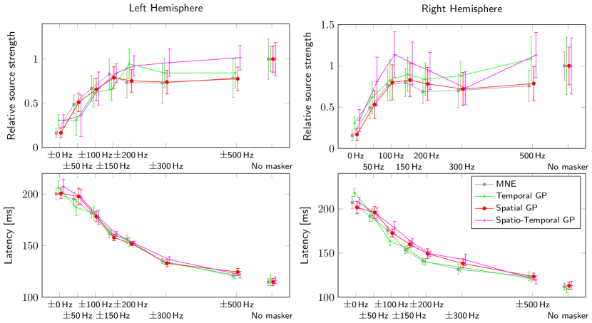
Figure 7 summarizes our empirical findings. It shows M100 sources strengths and peak times modulated by masker type. Note that as we successively consider the independent, temporal, spatial and spatio-temporal models, SEM reduces and curves appear to become more consistent. This further strengthens our belief that spatio-temporal regularization is important for obtaining reliable source estimates.
Acknowledgements
This work was supported by the Academy of Finland grant numbers 266940 and 273475, the Netherlands Organization for Scientific Research (NWO) grant numbers 612.001.211 and 639.072.513, and the Finnish Cultural Foundation. We acknowledge the computational resources provided by the Aalto Science-IT project.
Appendix A Proof of Theorem 2.2
Proof of the expression in Equation (11).
The following derivation is analogous to the GP formulation for grids presented by Saatçi (2012) except for the additional linear transformation via the lead field matrix in our setting. As stated in Equation (6), the expression for the mean is given by . Using the equivalence and space-time separability , the mean can be written as
| (25) |
The transpose is distributive over the Kronecker product,
| (26) |
Using the mixed-product property of the Kronecker product
| (27) |
and the eigendecompositions and ,
| (28) |
where . This is a diagonal (non-singular) matrix.
Vectorization combined with a multiplying Kronecker product has the convenient property that if and are nonsingular, (see, e.g., Horn & Johnson, 2012). Applying this property once gives us
| (29) |
The second parentheses contains just a product of a diagonal matrix times a long vector. In order to tidy up the notation, we define a matrix such that . Element-wise this is , where and .
| (30) |
where ‘’ denotes the element-wise Hadamard product , such that . We apply the product-vectorization property once more to obtain
| (31) |
If and are vectors, we can drop the vectorization, and we obtain the result in Theorem 2.2.∎
Proof of the expression in Equation (12).
From Equation (7), we focus on the latter part, denoted by and write
| (32) |
where we apply the distributivity of the transpose in the Kronecker product and the mixed-product property
| (33) |
Again, we consider the eigendecompositions and and get
| (34) |
This is an inner product, and regrouping the the terms gives us
| (35) |
That is, we get the result in Theorem 2.2.∎
References
- Andersen et al. (2015) Andersen, M. R., Vehtari, A., Winther, O., & Hansen, L. K. (2015). Bayesian inference for spatio-temporal spike and slab priors. arXiv preprint arXiv:1509.04752 [stat.ML], .
- Andersen et al. (2014) Andersen, M. R., Winther, O., & Hansen, L. K. (2014). Bayesian inference for structured spike and slab priors. In Advances in Neural Information Processing Systems (pp. 1745–1753).
- Arfken & Weber (2001) Arfken, G. B., & Weber, H. J. (2001). Mathematical Methods for Physicists. (5th ed.). New York: Academic press.
- Auranen et al. (2005) Auranen, T., Nummenmaa, A., Hämäläinen, M. S., Jääskeläinen, I. P., Lampinen, J., Vehtari, A., & Sams, M. (2005). Bayesian analysis of the neuromagnetic inverse problem with -norm priors. NeuroImage, 26, 870–884.
- Babadi et al. (2014) Babadi, B., Obregon-Henao, G., Lamus, C., Hämäläinen, M. S., Brown, E. N., & Purdon, P. L. (2014). A subspace pursuit-based iterative greedy hierarchical solution to the neuromagnetic inverse problem. NeuroImage, 87, 427–443.
- Bahramisharif et al. (2012) Bahramisharif, A., Van Gerven, M. A., Schoffelen, J.-M., Ghahramani, Z., & Heskes, T. (2012). The dynamic beamformer. In Machine Learning and Interpretation in Neuroimaging (pp. 148–155). Springer.
- Baillet & Garnero (1997) Baillet, S., & Garnero, L. (1997). A Bayesian approach to introducing anatomo-functional priors in the EEG/MEG inverse problem. IEEE Transactions on Biomedical Engineering, 44, 374–385.
- Baillet et al. (2001) Baillet, S., Mosher, J. C., & Leahy, R. M. (2001). Electromagnetic brain mapping. IEEE Signal Processing Magazine, 18, 14–30.
- Bishop (2006) Bishop, C. M. (2006). Pattern Recognition and Machine Learning. New York: Springer.
- Bolstad et al. (2009) Bolstad, A., Van Veen, B., & Nowak, R. (2009). Space–time event sparse penalization for magneto-/electroencephalography. NeuroImage, 46, 1066–1081.
- Castaño-Candamil et al. (2015) Castaño-Candamil, S., Höhne, J., Martínez-Vargas, J.-D., An, X.-W., Castellanos-Domínguez, G., & Haufe, S. (2015). Solving the EEG inverse problem based on space–time–frequency structured sparsity constraints. NeuroImage, 118, 598–612.
- Chen et al. (2015) Chen, X., Särkkä, S., & Godsill, S. (2015). A Bayesian particle filtering method for brain source localisation. Accepted for publication in Digital Signal Processing, .
- Cohen (1972) Cohen, D. (1972). Magnetoencephalography: Detection of the brain’s electrical activity with a superconducting magnetometer. Science, 175, 664–666.
- Cotter et al. (2005) Cotter, S., Rao, B., & Kreutz-Delgado, K. (2005). Sparse solutions to linear inverse problems with multiple measurement vectors. IEEE Transactions on Signal Processing, 53, 2477–2488.
- Dale et al. (2000) Dale, A. M., Liu, A. K., Fischl, B. R., Buckner, R. L., Belliveau, J. W., Lewine, J. D., & Halgren, E. (2000). Dynamic statistical parametric mapping: Combining fMRI and MEG for high-resolution imaging of cortical activity. Neuron, 26, 55–67.
- Dannhauer et al. (2013) Dannhauer, M., Lämmel, E., Wolters, C. H., & Knösche, T. R. (2013). Spatio-temporal regularization in linear distributed source reconstruction from EEG/MEG: a critical evaluation. Brain Topography, 26, 229–246.
- Darvas et al. (2001) Darvas, F., Schmitt, U., Louis, A. K., Fuchs, M., Knoll, G., & Buchner, H. (2001). Spatio-temporal current density reconstruction (stCDR) from EEG/MEG-data. Brain Topography, 13, 195–207.
- Daunizeau et al. (2007) Daunizeau, J., Grova, C., Marrelec, G., Mattout, J., Jbabdi, S., Pélégrini-Issac, M., Lina, J.-M., & Benali, H. (2007). Symmetrical event-related EEG/fMRI information fusion in a variational Bayesian framework. NeuroImage, 36, 69–87.
- Daunizeau et al. (2006) Daunizeau, J., Mattout, J., Clonda, D., Goulard, B., Benali, H., & Lina, J.-M. (2006). Bayesian spatio-temporal approach for EEG source reconstruction: conciliating ecd and distributed models. IEEE Transactions on Biomedical Engineering, 53, 503–516.
- Freeden & Schreiner (1995) Freeden, W., & Schreiner, M. (1995). Non-orthogonal expansions on the sphere. Mathematical Methods in the Applied Sciences, 18, 83–120.
- Friston et al. (2008) Friston, K., Harrison, L., Daunizeau, J., Kiebel, S., Phillips, C., Trujillo-Barreto, N., Henson, R., Flandin, G., & Mattout, J. (2008). Multiple sparse priors for the M/EEG inverse problem. NeuroImage, 39, 1104–1120.
- Fuchs et al. (1999) Fuchs, M., Wagner, M., Köhler, T., & Wischmann, H.-A. (1999). Linear and nonlinear current density reconstructions. Journal of clinical Neurophysiology, 16, 267–295.
- Fukushima et al. (2015) Fukushima, M., Yamashita, O., Knösche, T. R., & Sato, M.-a. (2015). Meg source reconstruction based on identification of directed source interactions on whole-brain anatomical networks. NeuroImage, 105, 408–427.
- Galka et al. (2004) Galka, A., Yamashita, O., Ozaki, T., Biscay, R., & Valdés-Sosa, P. (2004). A solution tot the dynamical inverse problem of EEG generation using spatiotemporal Kalman filtering. NeuroImage, 23, 435–453.
- van Gerven et al. (2009) van Gerven, M., Cseke, B., Oostenveld, R., & Heskes, T. (2009). Bayesian source localization with the multivariate Laplace prior. In Advances in Neural Information Processing Systems (pp. 1901–1909). volume 22.
- Geselowitz (1970) Geselowitz, D. B. (1970). On the magnetic field generated outside an inhomogeneous volume conductor by internal current sources. IEEE Transactions on Magnetics, 6, 346–347.
- Gorodnitsky et al. (1995) Gorodnitsky, I. F., George, J. S., & Rao, B. D. (1995). Neuromagnetic source imaging with focuss: a recursive weighted minimum norm algorithm. Electroencephalography and Clinical Neurophysiology, 95, 231–251.
- Gramfort et al. (2012) Gramfort, A., Kowalski, M., & Hämäläinen, M. (2012). Mixed-norm estimates for the M/EEG inverse problem using accelerated gradient methods. Physics in Medicine and Biology, 57, 1937.
- Gramfort et al. (2013) Gramfort, A., Strohmeier, D., Haueisen, J., Hämäläinen, M. S., & Kowalski, M. (2013). Time-frequency mixed-norm estimates: Sparse M/EEG imaging with non-stationary source activations. NeuroImage, 70, 410–422.
- Greensite (2003) Greensite, F. (2003). The temporal prior in bioelectromagnetic source imaging problems. IEEE Transactions on Biomedical Engineering, 50, 1152–1159.
- Hämäläinen et al. (1993) Hämäläinen, M. S., Hari, R., Ilmoniemi, R., Knuutila, J., & Lounasmaa, O. V. (1993). Magnetoencephalography—Theory, instrumentation, and applications to noninvasive studies of the working human brain. Reviews of Modern Physics, 65, 413–497.
- Hämäläinen & Ilmoniemi (1994) Hämäläinen, M. S., & Ilmoniemi, R. (1994). Interpreting magnetic fields of the brain: Minimum norm estimates. Medical & Biological Engineering & Computing, 32, 35–42.
- Hari & Parkkonen (2015) Hari, R., & Parkkonen, L. (2015). The brain timewise: How timing shapes and supports brain function. Philosophical Transactions of the Royal Society of London B: Biological Sciences, 370, 20140170.
- Haufe et al. (2008) Haufe, S., Nikulin, V. V., Ziehe, A., Müller, K.-R., & Nolte, G. (2008). Combining sparsity and rotational invariance in EEG/MEG source reconstruction. NeuroImage, 42, 726–738.
- Haufe et al. (2011) Haufe, S., Tomioka, R., Dickhaus, T., Sannelli, C., Blankertz, B., Nolte, G., & Müller, K.-R. (2011). Large-scale EEG/MEG source localization with spatial flexibility. NeuroImage, 54, 851–859.
- Henson et al. (2010) Henson, R. N., Flandin, G., Friston, K. J., & Mattout, J. (2010). A parametric empirical Bayesian framework for fMRI-constrained MEG/EEG source reconstruction. Human Brain Mapping, 31, 1512–1531.
- Horn & Johnson (2012) Horn, R. A., & Johnson, C. R. (2012). Matrix Analysis. Cambridge University Press.
- Kauramäki et al. (2012) Kauramäki, J., Jääskeläinen, I. P., Hänninen, J. L., Auranen, T., Nummenmaa, A., Lampinen, J., & Sams, M. (2012). Two-stage processing of sounds explains behavioral performance variations due to changes in stimulus contrast and selective attention: An MEG study. PloS one, 7, e46872.
- Lamus et al. (2012) Lamus, C., Hämäläinen, M. S., Temereanca, S., Brown, E. N., & Purdon, P. L. (2012). A spatiotemporal dynamic distributed solution to the MEG inverse problem. NeuroImage, 63, 894–909.
- Langers & van Dijk (2012) Langers, D. R. M., & van Dijk, P. (2012). Mapping the tonotopic organization in human auditory cortex with minimally salient acoustic stimulation. Cerebral Cortex, 22, 2024–2038.
- Limpiti et al. (2009) Limpiti, T., Van Veen, B. D., Attias, H. T., & Nagarajan, S. S. (2009). A spatiotemporal framework for estimating trial-to-trial amplitude variation in event-related MEG/EEG. IEEE Transactions on Biomedical Engineering, 56, 633–645.
- Lina et al. (2014) Lina, J., Chowdhury, R., Lemay, E., Kobayashi, E., & Grova, C. (2014). Wavelet-based localization of oscillatory sources from magnetoencephalography data. IEEE Transactions on Biomedical Engineering, 61, 2350–2364.
- Litvak & Friston (2008) Litvak, V., & Friston, K. (2008). Electromagnetic source reconstruction for group studies. NeuroImage, 42, 1490–1498.
- Liu et al. (2015) Liu, K., Yu, Z. L., Wu, W., Gu, Z., & Li, Y. (2015). STRAPS: A fully data-driven spatio-temporally regularized algorithm for M/EEG patch source imaging. International Journal of Neural Systems, (p. 1550016).
- Long et al. (2011) Long, C. J., Purdon, P. L., Temereanca, S., Desai, N. U., Hämäläinen, M. S., & Brown, E. N. (2011). State-space solutions to the dynamic magnetoencephalography inverse problem using high performance computing. The Annals of Applied Statistics, 5, 1207.
- Lucka et al. (2012) Lucka, F., Pursiainen, S., Burger, M., & Wolters, C. H. (2012). Hierarchical Bayesian inference for the EEG inverse problem using realistic FE head models: Depth localization and source separation for focal primary currents. NeuroImage, 61, 1364–1382.
- Mattout et al. (2006) Mattout, J., Phillips, C., Penny, W. D., Rugg, M. D., & Friston, K. J. (2006). MEG source localization under multiple constraints: An extended Bayesian framework. NeuroImage, 30, 753–767.
- Mosher & Leahy (1998) Mosher, J. C., & Leahy, R. M. (1998). Recursive MUSIC: A framework for EEG and MEG source localization. IEEE Transactions on Biomedical Engineering, 45, 1342–1354.
- Nummenmaa et al. (2007) Nummenmaa, A., Auranen, T., Hämäläinen, M. S., Jääskeläinen, I. P., Lampinen, J., Sams, M., & Vehtari, A. (2007). Hierarchical Bayesian estimates of distributed MEG sources: Theoretical aspects and comparison of variational and MCMC methods. NeuroImage, 35, 669–685.
- Ou et al. (2009) Ou, W., Hämäläinen, M. S., & Golland, P. (2009). A distributed spatio-temporal EEG/MEG inverse solver. NeuroImage, 44, 932–946.
- Ou et al. (2010) Ou, W., Nummenmaa, A., Ahveninen, J., Belliveau, J. W., Hämäläinen, M. S., & Golland, P. (2010). Multimodal functional imaging using fMRI-informed regional EEG/MEG source estimation. NeuroImage, 52, 97–108.
- Pascual-Marqui (2002) Pascual-Marqui, R. D. (2002). Standardized low-resolution brain electromagnetic tomography (sLORETA): Technical details. In Methods and Findings in Experimental and Clinical Pharmacology (pp. 5–12). volume 24 Suppl D.
- Pascual-Marqui et al. (1994) Pascual-Marqui, R. D., Michel, C. M., & Lehmann, D. (1994). Low resolution electromagnetic tomography: A new method for localizing electrical activity in the brain. International Journal of Psychophysiology, 18, 49–65.
- Petrov (2012) Petrov, Y. (2012). Harmony: EEG/MEG linear inverse source reconstruction in the anatomical basis of spherical harmonics. PloS one, 7, e44439.
- Phillips et al. (2005) Phillips, C., Mattout, J., Rugg, M. D., Maquet, P., & Friston, K. J. (2005). An empirical Bayesian solution to the source reconstruction problem in EEG. NeuroImage, 24, 997–1011.
- Pirondini et al. (2012) Pirondini, E., Babadi, B., Lamus, C., Brown, E. N., & Purdon, P. (2012). A spatially-regularized dynamic source localization algorithm for EEG. In International Conference of the IEEE Engineering in Medicine and Biology Society (EMBC) (pp. 6752–6755). IEEE.
- Rasmussen & Williams (2006) Rasmussen, C. E., & Williams, C. K. I. (2006). Gaussian Processes for Machine Learning. The MIT Press, Cambridge, Massachusetts.
- Saatçi (2012) Saatçi, Y. (2012). Scalable Inference for Structured Gaussian Process Models. Ph.D. thesis University of Cambridge Cambridge, UK.
- Särkkä et al. (2013) Särkkä, S., Solin, A., & Hartikainen, J. (2013). Spatio-temporal learning via infinite-dimensional Bayesian filtering and smoothing. IEEE Signal Processing Magazine, 30, 51–61.
- Sarvas (1987) Sarvas, J. (1987). Basic mathematical and electromagnetic concepts of the biomagnetic inverse problem. Physics in Medicine and Biology, 32, 11–22.
- Sato et al. (2004) Sato, M.-a., Yoshioka, T., Kajihara, S., Toyama, K., Goda, N., Doya, K., & Kawato, M. (2004). Hierarchical Bayesian estimation for MEG inverse problem. NeuroImage, 23, 806–826.
- Serinaĝaoĝlu et al. (2005) Serinaĝaoĝlu, Y., Brooks, D. H., & MacLeod, R. S. (2005). Bayesian solutions and performance analysis in bioelectric inverse problems. IEEE Transactions on Biomedical Engineering, 52, 1009–1020.
- Sorrentino et al. (2009) Sorrentino, A., Parkkonen, L., Pascarella, A., Campi, C., & Piana, M. (2009). Dynamical MEG source modeling with multi-target Bayesian filtering. Human Brain Mapping, 30, 1911–1921.
- Stahlhut et al. (2011) Stahlhut, C., Mørup, M., Winther, O., & Hansen, L. K. (2011). Simultaneous EEG source and forward model reconstruction (SOFOMORE) using a hierarchical Bayesian approach. Journal of Signal Processing Systems, 65, 431–444.
- Tarantola (2004) Tarantola, A. (2004). Inverse Problem Theory and Methods for Model Parameter Estimation. SIAM.
- Tian et al. (2012) Tian, T. S., Huang, J. Z., Shen, H., Li, Z. et al. (2012). A two-way regularization method for MEG source reconstruction. The Annals of Applied Statistics, 6, 1021–1046.
- Trujillo-Barreto et al. (2008) Trujillo-Barreto, N. J., Aubert-Vázquez, E., & Penny, W. D. (2008). Bayesian M/EEG source reconstruction with spatio-temporal priors. NeuroImage, 39, 318–335.
- Trujillo-Barreto et al. (2004) Trujillo-Barreto, N. J., Aubert-Vázquez, E., & Valdés-Sosa, P. A. (2004). Bayesian model averaging in EEG/MEG imaging. NeuroImage, 21, 1300–1319.
- Uutela et al. (1999) Uutela, K., Hämäläinen, M., & Somersalo, E. (1999). Visualization of magnetoencephalographic data using minimum current estimates. NeuroImage, 10, 173–180.
- Valdés-Sosa et al. (2009) Valdés-Sosa, P. A., Vega-Hernández, M., Sánchez-Bornot, J. M., Martínez-Montes, E., & Bobes, M. A. (2009). EEG source imaging with spatio-temporal tomographic nonnegative independent component analysis. Human Brain Mapping, 30, 1898–1910.
- van Veen et al. (1997) van Veen, B. D., van Drongelen, W., Yuchtman, M., & Suzuki, A. (1997). Localization of brain electrical activity via linearly constrained minimum variance spatial filtering. IEEE Transactions on Bio-Medical Engineering, 44, 867–880.
- Wipf & Nagarajan (2009) Wipf, D., & Nagarajan, S. (2009). A unified Bayesian framework for MEG/EEG source imaging. NeuroImage, 44, 947–966.
- Wipf et al. (2010) Wipf, D. P., Owen, J. P., Attias, H. T., Sekihara, K., & Nagarajan, S. S. (2010). Robust Bayesian estimation of the location, orientation, and time course of multiple correlated neural sources using MEG. NeuroImage, 49, 641–655.
- Woolrich et al. (2013) Woolrich, M. W., Baker, A., Luckhoo, H., Mohseni, H., Barnes, G., Brookes, M., & Rezek, I. (2013). Dynamic state allocation for MEG source reconstruction. NeuroImage, 77, 77–92.
- Yamashita et al. (2004) Yamashita, O., Galka, A., Ozaki, T., Biscay, R., & Valdes-Sosa, P. (2004). Recursive penalized least squares solution for dynamical inverse problems of EEG generation. Human Brain Mapping, 21, 221–235.
- Zhang & Rao (2011) Zhang, Z., & Rao, B. D. (2011). Sparse signal recovery with temporally correlated source vectors using sparse Bayesian learning. IEEE Journal of Selected Topics in Signal Processing, 5, 912–926.
- Zumer et al. (2007) Zumer, J. M., Attias, H. T., Sekihara, K., & Nagarajan, S. S. (2007). A probabilistic algorithm integrating source localization and noise suppression for MEG and EEG data. NeuroImage, 37, 102–115.