Certified Descent Algorithm for shape optimization driven by fully-computable a posteriori error estimators

Abstract

In this paper we introduce a novel certified shape optimization strategy - named Certified Descent Algorithm (CDA) - to account for the numerical error introduced by the Finite Element approximation of the shape gradient. We present a goal-oriented procedure to derive a certified upper bound of the error in the shape gradient and we construct a fully-computable, constant-free a posteriori error estimator inspired by the complementary energy principle. The resulting CDA is able to identify a genuine descent direction at each iteration and features a reliable stopping criterion. After validating the error estimator, some numerical simulations of the resulting certified shape optimization strategy are presented for the well-known inverse identification problem of Electrical Impedance Tomography.

Keywords: Shape optimization; A posteriori error estimator; Certified Descent Algorithm; Electrical Impedance Tomography

1 Introduction

Shape optimization is a class of optimization problems in which the objective functional depends on the shape of the domain in which a Partial Differential Equation (PDE) is formulated and on the solution of the PDE itself. Thus, we may view these problems as PDE-constrained optimization problems of a shape-dependent functional, the domain being the optimization variable and the PDE being the constraint. This class of problems has been tackled in the literature using both gradient-based and gradient-free methods and in this work we consider a strategy issue of the former group by computing the so-called shape gradient.

In most applications, the differential form of the objective functional with respect to the shape depends on the solution of a PDE which usually can only be solved approximately by means of a discretization strategy like the Finite Element Method. The approximation of the governing equation for the phenomenon under analysis introduces an uncertainty which may prevent the shape gradient from being strictly negative along the identified descent direction, that is, the approximated direction may not lead to any improvement of the objective functional we are trying to optimize. Moreover, due to the aforementioned approximation, stopping criteria based on the norm of the shape gradient may never be fulfilled if the a priori given tolerance is too small with respect to the chosen discretization. Within this framework, a posteriori error estimators provide useful information to improve gradient-based algorithms for shape optimization.

Several works in the literature have highlighted the great potential of coupling a posteriori error estimators to shape optimization algorithms. In the pioneering work [7], the authors identify two different sources for the numerical error: on the one hand, the error arising from the approximation of the differential problem and on the other hand, the error due to the approximation of the geometry. Starting from this observation, Banichuk et al. present a first attempt to use the information on the discretization of the differential problem provided by a recovery-based estimator and the error arising from the approximation of the geometry to develop an adaptive shape optimization strategy. This work has been later extended by Morin et al. in [28], where the adaptive discretization of the governing equations by means of the Adaptive Finite Element Method is linked to an adaptive strategy for the approximation of the geometry. The authors derive estimators of the numerical error that are later used to drive an Adaptive Sequential Quadratic Programming algorithm to appropriately refine and coarsen the computational mesh. Several other authors have used adaptive techniques for the approximation of PDE’s in order to improve the accuracy of the solution and obtain better final configurations in optimal structural design problems. We refer to [25, 36, 3, 34] for some examples. We remark that in all these works, a posteriori estimators only provide qualitative information about the numerical error due to the discretization of the problems and are essentially used to drive mesh adaptation procedures. To the best of our knowledge, no guaranteed fully-computable estimate has been investigated and the error in the shape gradient itself is not accounted for, thus preventing reliable stopping criteria to be derived.

In the present paper, the derivation of a fully-computable upper bound for the error in the shape gradient is tackled. We neglect the contribution of the approximation of the geometry and we focus on the error arising from the discretization of the governing equation. The quantitative estimate of the error due to the numerical approximation of the shape gradient allows to identify a genuine descent direction and to introduce a reliable stopping criterion for the overall optimization strategy. We propose a novel shape optimization strategy - named Certified Descent Algorithm (CDA) - that generates a sequence of minimizing shapes by certifying at each iteration the descent direction to be genuine and automatically stops when a reliable stopping criterion is fulfilled.

The rest of the paper is organized as follows. First, we introduce the general framework of shape optimization and shape identification problems and the so-called Boundary Variation Algorithm (Section 2). In section 3, we account for the discretization error in the Quantity of Interest using the framework presented in [29]. Then, we introduce the resulting Certified Descent Algorithm that couples the a posteriori error estimator and the Boundary Variation Algorithm to derive a genuine descent direction for the shape optimization problem (Section 4). In section 5, we present the application of the Certified Descent Algorithm to the inverse problem of Electrical Impedance Tomography (EIT): after introducing the formulation of the identification problem as a shape optimization problem, we derive a fully-computable upper bound of the error in the shape gradient using the complementary energy principle. Eventually, in section 6 we present some numerical tests of the application of CDA to the EIT problem and section 7 summarizes our results.

2 Shape optimization and shape identification problems

We consider an open domain $\Omega\subset\mathbb{R}^{d}$ ($d\geq 2$) with Lipschitz boundary $\partial\Omega$. Let $V_{\Omega}$ be a separable Hilbert space depending on $\Omega$, we define $u_{\Omega}\in V_{\Omega}$ to be the solution of a state equation which is a linear PDE in the domain $\Omega$:

$$a_{\Omega}(u_{\Omega},\delta u)=F_{\Omega}(\delta u)\qquad\forall\delta u\in V_{\Omega}$$ (2.1)

where $a_{\Omega}(\cdot,\cdot):V_{\Omega}\times V_{\Omega}\rightarrow\mathbb{R}$ is a continuous bilinear form satisfying the inf-sup condition

$$\adjustlimits{\inf}_{w\in V_{\Omega}}{\sup}_{v\in V_{\Omega}}\frac{a_{\Omega}(v,w)}{\|v\|\|w\|}=\adjustlimits{\inf}_{v\in V_{\Omega}}{\sup}_{w\in V_{\Omega}}\frac{a_{\Omega}(v,w)}{\|v\|\|w\|}>0$$

and $F_{\Omega}(\cdot)$ is a continuous linear form on $V_{\Omega}$, both of them depending on $\Omega$. Under these assumptions, problem (2.1) has a unique solution $u_{\Omega}$.

We introduce a cost functional $J(\Omega)=j(\Omega,u_{\Omega})$ which depends on the domain $\Omega$ itself and on the solution $u_{\Omega}$ of the state equation. We consider the following shape optimization problem

$$\min_{\Omega\in\mathcal{U}_{\text{ad}}}J(\Omega)$$ (2.2)

where $\mathcal{U}_{\text{ad}}$ is the set of admissible domains in $\mathbb{R}^{d}$. Within this framework, problem (2.2) may be viewed as a PDE-constrained optimization problem, in which we aim at minimizing the functional $j(\Omega,u)$ under the constraint $u=u_{\Omega}$, that is the minimizer $u$ is solution of the state equation (2.1).
In the following subsections, we recall the notion of shape gradient of $J(\Omega)$ in the direction $\theta$ and we apply the Steepest Descent Method to the shape optimization problem (2.2).

2.1 Differentiation with respect to the shape

Let $X\subset W^{1,\infty}(\Omega;\mathbb{R}^{d})$ be a Banach space and $\theta\in X$ be an admissible smooth deformation of $\Omega$. The cost functional $J(\Omega)$ is said to be $X$-differentiable at $\Omega\in\mathcal{U}_{\text{ad}}$ if there exists a continuous linear form $dJ(\Omega)$ on $X$ such that $\forall\theta\in X$

$$J((\operatorname{Id}+\theta)\Omega)=J(\Omega)+\langle dJ(\Omega),\theta\rangle+o(\theta).$$

Several approaches are feasible to compute the shape gradient. Here we briefly recall the fast derivation method by Céa [11] and the material derivative approach [37]. Let us introduce the Lagrangian functional, defined for every admissible open set $\Omega$ and every $u,\ p\in V_{\Omega}$ by

$$\mathcal{L}(\Omega,u,p)=j(\Omega,u)+a_{\Omega}(u,p)-F_{\Omega}(p).$$ (2.3)

Let $p_{\Omega}\in V_{\Omega}$ be the solution of the so-called adjoint problem, that is

$$a_{\Omega}(\delta p,p_{\Omega})+\left\langle\frac{\partial j}{\partial u}(\Omega,u_{\Omega}),\delta p\right\rangle=0\qquad\forall\delta p\in V_{\Omega}.$$ (2.4)

By applying the fast derivation method by Céa, we get the following expression of the shape gradient:

$$\langle dJ(\Omega),\theta\rangle=\left\langle\frac{\partial\mathcal{L}}{\partial\Omega}(\Omega,u_{\Omega},p_{\Omega}),\theta\right\rangle.$$ (2.5)

An alternative procedure to compute the shape gradient relies on the definition of a diffeomorphism $\varphi:\mathbb{R}^{d}\rightarrow\mathbb{R}^{d}$ such that for every admissible set $\Omega$

$$\Omega_{\varphi}\coloneqq\varphi(\Omega).$$

Moreover, all functions $u,\ p\in V_{\Omega}$ defined on the reference domain $\Omega$ may be mapped to the deformed domain $\Omega_{\varphi}$ by

$$u_{\varphi}\coloneqq u\circ\varphi^{-1}\qquad\text{and}\qquad p_{\varphi}\coloneqq p\circ\varphi^{-1}.$$

We admit that $u\mapsto u_{\varphi}$ is a one-to-one map between $V_{\Omega}$ and $V_{\varphi(\Omega)}$. The Lagrangian (2.3) is said to admit a material derivative if there exists a linear form $\frac{\partial\mathcal{L}}{\partial\varphi}$ such that

$$\mathcal{L}(\Omega_{\varphi},u_{\varphi},p_{\varphi})=\mathcal{L}(\Omega,u,p)+\left\langle\frac{\partial\mathcal{L}}{\partial\varphi}(\Omega,u,p),\theta\right\rangle+o(\theta)$$

where $\varphi=\operatorname{Id}+\theta$. Provided that $u_{\varphi}$ is differentiable with respect to $\varphi$ at $\varphi=\operatorname{Id}$ in $V_{\varphi(\Omega)}$, from the fast derivation method of Céa we obtain the following expression for the shape gradient:

$$\langle dJ(\Omega),\theta\rangle=\left\langle\frac{\partial\mathcal{L}}{\partial\varphi}(\Omega,u_{\Omega},p_{\Omega}),\theta\right\rangle.$$ (2.6)

A variant of the latter method consists in computing the shape gradient via the Lagrangian formulation without explicitly constructing the material derivative of the state and adjoint solutions. We refer to [27] for additional information about this approach.

Volumetric and surface expressions of the shape gradient

The most common approach in the literature to compute the shape gradient is based on an Eulerian point of view and leads to a surface expression of the shape gradient.
The main advantage of this method relies on the fact that the boundary representation intuitively provides an explicit expression for the descent direction. Let us assume that the shape gradient has the following form

$$\langle dJ(\Omega),\theta\rangle=\int_{\partial\Omega}{h\theta\cdot nds}$$

then $\theta=-hn$  on  $\partial\Omega$ is a descent direction. Moreover, by Hadamard-Zolésio structure theorem it is well-known that the shape gradient is carried on the boundary of the shape [14] and using this approach the descent direction has to be defined only on $\partial\Omega$. Nevertheless, if the boundary datum of the state problem is not sufficiently smooth, the surface expression of the shape gradient may not exist or the descent direction $\theta$ may suffer from poor regularity.
Starting from the surface representation of the shape gradient, it is possible to derive a volumetric expression as well. Though the two expressions are equivalent in a continuous framework, they usually are not when considering their numerical counterparts, e.g. their Finite Element approximations: as a matter of fact, in [22] Hiptmair et al. prove that the volumetric formulation generally provides better accuracy when using the Finite Element Method. Moreover, we may be able to derive the volumetric expression of the shape gradient even when its boundary representation fails to exist.
In this work, we consider the volumetric expression of the shape gradient in order to take advantage of the better accuracy it provides from a numerical point of view and to construct an estimator of the error in a Quantity of Interest using the procedure described by Oden and Prudhomme in [29].
We remark that in order to derive a descent direction $\theta$ on $\Omega$ from the volumetric expression of the shape gradient, an additional variational problem has to be solved, as described in next subsection.

2.2 The Boundary Variation Algorithm

From now on, we consider $X$ to be a Hilbert space. Starting from the formulation (2.6), we seek a descent direction for the functional $J(\Omega)$. For this purpose, we solve an additional variational problem and we seek $\theta\in X$ such that

$$(\theta,\delta\theta)_{X}+\langle dJ(\Omega),\delta\theta\rangle=0\qquad\forall\delta\theta\in X.$$ (2.7)

Remark 2.1.

The choice of the scalar product in (2.7) is a key point for the development of an efficient shape optimization method. In [6], the authors propose the so-called traction method to get rid of some irregularity issues in shape optimization problems. This approach is based on the regularization of the descent direction by means of a scalar product inspired by the linear elasticity equation. In recent years, a comparison of the $L^{2}$, $H^{1}$ and $H^{-1}$ scalar products defined on a surface was presented [15] but, as the authors state, the best choice is strongly dependent on the application of interest.

In this section, we present the application of the Steepest Descent Method to a shape optimization problem. After computing the solution of the state equation, we solve the adjoint problem to derive the expression of the shape gradient. Then, a descent direction is identified through (2.7) and is used to deform the domain. The resulting shape optimization strategy is known in the literature as Boundary Variation Algorithm [4] and is sketched in script 1.

Algorithm 1: Continuous gradient method - The Boundary Variation Algorithm

⬇

Given the domain $\Omega_{0}$, set $\ell=0$ and iterate:

1. Compute the solution $u_{\Omega_{\ell}}$ of the state equation;

2. Compute the solution $p_{\Omega_{\ell}}$ of the adjoint equation;

3. Compute a descent direction $\theta_{\ell}\in X$ solving $(\theta_{\ell},\delta\theta)_{X}+\langle dJ(\Omega_{\ell}),\delta\theta\rangle=0\quad\forall\delta\theta\in X$;

4. Identify an admissible step $\mu_{\ell}$;

5. Update the domain $\Omega_{\ell+1}=(\operatorname{Id}+\mu_{\ell}\theta_{\ell})\Omega_{\ell}$;

6. While $|\langle dJ(\Omega_{\ell}),\theta_{\ell}\rangle|>\texttt{tol}$, $\ell=\ell+1$ and repeat.

We remark that this method relies on the computation at each iteration of a direction $\theta$ such that the shape gradient of the objective functional in this direction is strictly negative, that is we seek $\theta$ such that $\langle dJ(\Omega),\theta\rangle<0$. In next subsection, we discuss the modifications that occur when moving from the continuous to the discretized formulation of the problems and consequently the conditions that the discretization of $\theta$ has to fulfill in order to be a genuine descent direction for the functional $J(\Omega)$.

2.3 The discretized Boundary Variation Algorithm

Let us denote by $u_{\Omega}^{h}$ and $p_{\Omega}^{h}$ the approximations of the state and adjoint equations arising from a Finite Element discretization. The discretized direction $\theta^{h}\in X$ is obtained by solving problem (2.8)

$$(\theta^{h},\delta\theta)_{X}+\langle d_{h}J(\Omega),\delta\theta\rangle=0\qquad\forall\delta\theta\in X$$ (2.8)

where $\langle d_{h}J(\Omega),\delta\theta\rangle$ reads as follows:

$$\langle d_{h}J(\Omega),\delta\theta\rangle\coloneqq\left\langle\frac{\partial\mathcal{L}}{\partial\varphi}(\Omega,u_{\Omega}^{h},p_{\Omega}^{h}),\delta\theta\right\rangle.$$ (2.9)

The discretized version of the Boundary Variation Algorithm is derived by substituting the continuous functions $u_{\Omega}$, $p_{\Omega}$ with their approximations $u_{\Omega}^{h}$, $p_{\Omega}^{h}$ and $\theta$  with  $\theta^{h}$:

Algorithm 2: Discretized gradient method - The discretized Boundary Variation Algorithm

⬇

Given the domain $\Omega_{0}$, set $\ell=0$ and iterate:

1. Compute the solution $u_{\Omega_{\ell}}^{h}$ of the state equation;

2. Compute the solution $p_{\Omega_{\ell}}^{h}$ of the adjoint equation;

3. Compute a descent direction $\theta_{\ell}^{h}\in X$ solving $(\theta_{\ell}^{h},\delta\theta)_{X}+\langle d_{h}J(\Omega_{\ell}),\delta\theta\rangle=0\quad\forall\delta\theta\in X$;

4. Identify an admissible step $\mu_{\ell}$;

5. Update the domain $\Omega_{\ell+1}=(\operatorname{Id}+\mu_{\ell}\theta_{\ell}^{h})\Omega_{\ell}$;

6. While $|\langle d_{h}J(\Omega_{\ell}),\theta_{\ell}^{h}\rangle|>\texttt{tol}$, $\ell=\ell+1$ and repeat.

We remark that due to the numerical error introduced by the Finite Element discretization, even though $\langle d_{h}J(\Omega),\theta^{h}\rangle<0$,  $\theta^{h}$ is not necessarily a genuine descent direction for the functional $J(\Omega)$. Moreover, it is important to notice that the stopping criterion (Algorithm 2 - step 6) will usually not be fulfilled if the required tolerance tol is too sharp with respect to the chosen discretization.
In order to bypass these issues, in the following sections we present a strategy to account for the error introduced by the approximation of the shape gradient. This results in a certification procedure that allows to verify whether a given direction is a genuine descent direction for the functional $J(\Omega)$ or not.

2.4 Certification procedure for a genuine descent direction

In this section we introduce the notion of certified descent direction, that is a direction which is verified to be a genuine descent direction for the functional $J(\Omega)$. As previously stated, a genuine descent direction $\theta$ is such that

$$\langle dJ(\Omega),\theta\rangle<0.$$ (2.10)

When moving from the continuous to the Finite Element framework, an approximation of the shape gradient is introduced (cf. definition (2.9)) and consequently a numerical error appears. We define the error in the shape gradient $E^{h}$ as follows:

$$E^{h}\coloneqq\langle dJ(\Omega)-d_{h}J(\Omega),\theta^{h}\rangle.$$ (2.11)

By observing that $\langle dJ(\Omega),\theta^{h}\rangle=\langle d_{h}J(\Omega),\theta^{h}\rangle+E^{h}$, we get that a discretized direction $\theta^{h}$ is a descent direction for the objective functional $J(\Omega)$ if

$$\langle d_{h}J(\Omega),\theta^{h}\rangle+E^{h}<0.$$ (2.12)

By construction, we seek $\theta^{h}$ such that $\langle d_{h}J(\Omega),\theta^{h}\rangle<0$. Nevertheless, this condition does not imply that $\theta^{h}$ is a genuine descent direction for $J(\Omega)$ since the quantity $E^{h}$ in (2.12) may be either positive or negative. In order to derive a relationship that stands independently from the sign of $E^{h}$ and since no a priori information on the aforementioned sign is available, we modify (2.12) by introducing the absolute value of $E^{h}$:

$$\langle d_{h}J(\Omega),\theta^{h}\rangle+E^{h}<\langle d_{h}J(\Omega),\theta^{h}\rangle+|E^{h}|<0.$$ (2.13)

Let $\overline{E}$ be the upper bound of the quantity $|E^{h}|$. From (2.13), we derive the following condition for the certification procedure: we seek $\theta^{h}$ such that

$$\langle d_{h}J(\Omega),\theta^{h}\rangle+\overline{E}<0.$$ (2.14)

It is straightforward to observe that if $\theta^{h}$ fulfills (2.14), then it verifies (2.10) as well. Thus, a direction $\theta^{h}$ fulfilling condition (2.14) is said to be certified because it is guaranteed that the functional $J(\Omega)$ decreases along $\theta^{h}$. We remark that the criterion (2.14) ensures that $\theta^{h}$ is a genuine descent direction, whether it is the solution of equation (2.8) or not. In particular, this also stands when the latter problem is only solved approximately.
In the following section, we present a strategy to construct a fully-computable guaranteed upper bound of the error in the approximation of the shape gradient in order to practically implement the certification procedure described above.

3 Numerical error in the shape gradient

In this section, we provide the detail of the technique used to derive an upper bound $\overline{E}$ of the error $|E^{h}|$ in the shape gradient. The strategy to estimate the a posteriori error in a Quantity of Interest (QoI) - namely, the shape gradient - is derived from the work [29] by Oden and Prudhomme. Basic idea relies on the definition of an adjoint problem whose right-hand side is the quantity whose error estimate is sought.

3.1 Bound for the approximation error of a linear functional

Here we briefly recall the aforementioned strategy by Oden and Prudhomme for the derivation of an a posteriori error estimate for a bounded linear functional $Q:V_{\Omega}\rightarrow\mathbb{R}$, also known as Quantity of Interest. Let $e_{u}\coloneqq u_{\Omega}-u_{\Omega}^{h}$ be the error between the function $u_{\Omega}$ solution of the state problem (2.1) and its Finite Element counterpart $u_{\Omega}^{h}$. We are interested in evaluating the target $Q(u_{\Omega})$ and the accuracy of its approximation $Q(u_{\Omega}^{h})$ is expressed via the following quantity:

$$E_{Q}\coloneqq Q(u_{\Omega})-Q(u_{\Omega}^{h})=Q(u_{\Omega}-u_{\Omega}^{h})=Q(e_{u})$$

where the first equality follows from the linearity of $Q$. In order to compute the error $Q(e_{u})$, we introduce the residue associated with the approximation of the state problem (2.1):

$$\mathcal{R}_{\Omega}^{u}(\delta u)\coloneqq F_{\Omega}(\delta u)-a_{\Omega}(u_{\Omega}^{h},\delta u).$$ (3.1)

Moreover, we recall that the error $e_{u}$ is solution of the so-called residual equation that reads

$$a_{\Omega}(e_{u},\delta u)=\mathcal{R}_{\Omega}^{u}(\delta u)\qquad\forall\delta u\in V_{\Omega}.$$ (3.2)

We highlight that (3.1) contains all the information related to the numerical error $e_{u}$, thus the evaluation of $Q(e_{u})$ reduces to the derivation of a relationship between $\mathcal{R}_{\Omega}^{u}$ and $Q(e_{u})$ itself. Hence we seek a so-called influence function that carries the information on the effect of the residue - i.e. the effect of the error $e_{u}$ - on the functional $Q$. Let us assume that there exists an influence function $r_{\Omega}$ such that $Q(e_{u})=\mathcal{R}_{\Omega}^{u}(r_{\Omega})$. We may identify $r_{\Omega}$ with its Riesz element and owing to (3.2), we get

$$Q(e_{u})=\mathcal{R}_{\Omega}^{u}(r_{\Omega})=a_{\Omega}(e_{u},r_{\Omega}).$$

By combining the above information we are able to derive the following Boundary Variation Problem - known as adjoint problem - to construct the influence function. In particular, we seek $r_{\Omega}\in V_{\Omega}$ such that

$$a_{\Omega}(\delta r,r_{\Omega})=Q(\delta r)\qquad\forall\delta r\in V_{\Omega}.$$ (3.3)

Existence and uniqueness of the solution $r_{\Omega}$ of the adjoint problem follow from the Lax-Milgram theorem. From a practical point of view, the solution of the aforementioned adjoint problem is only approximated - usually using the same method as for the state problem - and an additional error $e_{r}\coloneqq r_{\Omega}-r_{\Omega}^{h}$ is introduced. Hence, owing to the Galerkin orthogonality the evaluation of $Q(e_{u})$ reads as

$$Q(e_{u})=a_{\Omega}(e_{u},r_{\Omega})=a_{\Omega}(e_{u},r_{\Omega}-r_{\Omega}^{h})=a_{\Omega}(e_{u},e_{r}).$$ (3.4)

3.2 Variational formulation of the error in the shape gradient

Several works in the literature [18, 35] have dealt with an extension of the aforementioned framework to compute a bound of the approximation error in a target functional to the case of non-linear Quantities of Interest. To account for the error (2.11), we follow the approach proposed by these authors by performing a linearization of the functional whose error estimate is sought. Thus we rewrite the numerical error (2.11) in the shape gradient by introducing the linearized error $\widetilde{E}^{h}$:

$$E^{h}= \left\langle\frac{\partial\mathcal{L}}{\partial\varphi}(\Omega,u_{\Omega},p_{\Omega})-\frac{\partial\mathcal{L}}{\partial\varphi}(\Omega,u_{\Omega}^{h},p_{\Omega}^{h}),\theta^{h}\right\rangle$$ (3.5)

$$\simeq\frac{\partial^{2}\mathcal{L}}{\partial\varphi\partial u}(\Omega,u_{\Omega}^{h},p_{\Omega}^{h})[\theta^{h},u_{\Omega}-u_{\Omega}^{h}]+\frac{\partial^{2}\mathcal{L}}{\partial\varphi\partial p}(\Omega,u_{\Omega}^{h},p_{\Omega}^{h})[\theta^{h},p_{\Omega}-p_{\Omega}^{h}]\eqqcolon\widetilde{E}^{h}.$$

In order to compute an upper bound of the error (3.5), we introduce two adjoint problems, each of which is associated with one term on the right-hand side of (3.5). Thus, we seek $r_{\Omega},s_{\Omega}\in V_{\Omega}$ such that

$$a_{\Omega}(\delta r,r_{\Omega})=\frac{\partial^{2}\mathcal{L}}{\partial\varphi\partial u}(\Omega,u_{\Omega}^{h},p_{\Omega}^{h})[\theta^{h},\delta r]\qquad\forall\delta r\in V_{\Omega}$$ (3.6)

$$a_{\Omega}(\delta s,s_{\Omega})=\frac{\partial^{2}\mathcal{L}}{\partial\varphi\partial p}(\Omega,u_{\Omega}^{h},p_{\Omega}^{h})[\theta^{h},\delta s]\qquad\forall\delta s\in V_{\Omega}$$

We remark that in order for the aforementioned adjoint problems to be well-posed, their right-hand sides have to be linear and continuous forms on $V_{\Omega}$ and this motivates the linearization introduced in (3.5).

Let us denote by $r_{\Omega}^{h}$, $s_{\Omega}^{h}$ the approximations of the solutions $r_{\Omega}$, $s_{\Omega}$ of equations (3.6) arising from a Finite Element discretization. By plugging (3.6) into (3.5), we may derive the following upper bound $\overline{E}$ for the numerical error in the shape gradient:

$$|E^{h}|\simeq|\widetilde{E}^{h}| \leq|a_{\Omega}(u_{\Omega}-u_{\Omega}^{h},r_{\Omega}-r_{\Omega}^{h})|+|a_{\Omega}(p_{\Omega}-p_{\Omega}^{h},s_{\Omega}-s_{\Omega}^{h})|$$ (3.7)

$$\leq\,|\!|\!|{{u_{\Omega}-u_{\Omega}^{h}}}|\!|\!|_{\Omega}\,|\!|\!|{{r_{\Omega}-r_{\Omega}^{h}}}|\!|\!|_{\Omega}+\,|\!|\!|{{p_{\Omega}-p_{\Omega}^{h}}}|\!|\!|_{\Omega}\,|\!|\!|{{s_{\Omega}-s_{\Omega}^{h}}}|\!|\!|_{\Omega}\eqqcolon\overline{E}$$

where $\,|\!|\!|{{\cdot}}|\!|\!|_{\Omega}$ is the energy-norm induced by the bilinear form $a_{\Omega}(\cdot,\cdot)$. The first inequality follows from triangle inequality and Galerkin orthogonality whereas the upper bound $\overline{E}$ is derived exploiting Cauchy-Schwarz inequality.

Remark 3.1.

In (3.7) we derived an upper bound for the numerical error in the linearized shape gradient and not in the shape gradient itself. For the rest of this paper, we will follow the framework in [18] by assuming the linearization error to be negligible and $\overline{E}$ to be an upper bound of the numerical error $E^{h}$ itself and not of its linearized version $\widetilde{E}^{h}$. In section 6.1, a validation of the error estimator is presented for the case of Electrical Impedance Tomography: we will verify that the linearization error is indeed negligible with respect to the error due to the Finite Element discretization and thus the previous assumption stands.

In order to fully compute the error estimator (3.7), we have to estimate the energy-norm of the error for:

• the state equation;

• the adjoint equation used to compute the shape gradient;

• the two adjoint equations associated with the Quantity of Interest.

Several strategies are possible to tackle these issues. In this paper, we propose a method inspired by the complementary energy principle which allows to derive fully-computable, constant-free estimators by solving an additional variational problem for each term under analysis in order to retrieve a flux estimate. These estimates are problem-dependent and will be detailed in section 5 when presenting the case of Electrical Impedance Tomography.

4 The Certified Descent Algorithm

We are now ready to introduce the novel Certified Descent Algorithm, arising from the coupling of the Boundary Variation Algorithm for shape optimization (Section 2.2) and the goal-oriented estimator for the error in the shape gradient (Section 3.2). In script 3, we present a variant of algorithm 1 that takes advantage of the previously introduced a posteriori estimator for the error in the shape gradient in order to bypass the issues due to the discretization of the problem.

First, the procedure constructs an initial computational domain. At each iteration, the algorithm solves the state and adjoint problems [steps 1 and 2] and computes a descent direction $\theta^{h}$ solving equation (2.8) [step 3]. Then, the adjoint problems (3.6) are solved and an upper bound of the numerical error in the shape gradient along the direction $\theta^{h}$ is computed [step 4]. If condition (2.14) is not fulfilled, the mesh is adapted in order to improve the error estimate. This procedure is iterated until the direction $\theta^{h}$ is a certified descent direction for $J(\Omega)$ [step 5]. Once a certified descent direction has been identified, we compute a step [step 6] such that the following Armijo condition is fulfilled: let us consider the iteration $\ell$, given $0<\alpha<1$ we use a backtracking strategy to identify the step $\mu_{\ell}\in\mathbb{R}^{+}$ such that

$$J\left(\left(\operatorname{Id}+\mu_{\ell}\theta_{\ell}^{h}\right)\Omega_{\ell}\right)\leq J\left(\Omega_{\ell}\right)+\alpha\mu_{\ell}\langle d_{h}J\left(\Omega_{\ell}\right),\theta_{\ell}^{h}\rangle.$$

An alternative bisection-based line search technique has been proposed by Morin et al. in [28].
Then the shape of the domain is updated according to the computed perturbation of the identity $\operatorname{Id}+\mu_{\ell}\theta_{\ell}^{h}$ [step 7]. Eventually, a novel stopping criterion is proposed [step 8] in order to use the information embedded in the error bound $\overline{E}$ to derive a reliable condition to end the evolution of the algorithm.

Algorithm 3: Discretized gradient method - The Certified Descent Algorithm

⬇

Given the domain $\Omega_{0}$, set $\ell=0$ and iterate:

1. Compute the solution $u_{\Omega_{\ell}}^{h}$ of the state equation;

2. Compute the solution $p_{\Omega_{\ell}}^{h}$ of the adjoint equation;

3. Compute a descent direction $\theta_{\ell}^{h}\in X$ solving $(\theta_{\ell}^{h},\delta\theta)_{X}+\langle d_{h}J(\Omega_{\ell}),\delta\theta\rangle=0\quad\forall\delta\theta\in X$;

4. Compute an upper bound $\overline{E}$ of the numerical error $|E^{h}|$:

(a) Compute the solutions $r_{\Omega_{\ell}}^{h}$ and $s_{\Omega_{\ell}}^{h}$ to estimate the error in the QoI;

(b) Compute $\overline{E}=\,|\!|\!|{{u_{\Omega_{\ell}}-u_{\Omega_{\ell}}^{h}}}|\!|\!|_{\Omega}\,|\!|\!|{{r_{\Omega_{\ell}}-r_{\Omega_{\ell}}^{h}}}|\!|\!|_{\Omega}+\,|\!|\!|{{p_{\Omega_{\ell}}-p_{\Omega_{\ell}}^{h}}}|\!|\!|_{\Omega}\,|\!|\!|{{s_{\Omega_{\ell}}-s_{\Omega_{\ell}}^{h}}}|\!|\!|_{\Omega}$;

5. If $\langle d_{h}J(\Omega_{\ell}),\theta_{\ell}^{h}\rangle+\overline{E}\geq 0$, refine the mesh and go to 1;

6. Identify an admissible step $\mu_{\ell}$;

7. Update the shape $\Omega_{\ell+1}=(\operatorname{Id}+\mu_{\ell}\theta_{\ell}^{h})\Omega_{\ell}$;

8. While $|\langle d_{h}J(\Omega_{\ell}),\theta_{\ell}^{h}\rangle|+\overline{E}>\texttt{tol}$, $\ell=\ell+1$ and repeat.

The advantage of the Certified Descent Algorithm is twofold. On the one hand, the computation of the upper bound of the numerical error in the shape gradient provides useful information to identify a certified descent direction at each iteration of the optimization algorithm and to construct a certified shape optimization strategy. On the other hand, the fully-computable and constant-free error estimator provides quantitative information to derive a reliable stopping criterion for the overall optimization procedure.

The novelty of algorithm 3 is the certification procedure that plays a crucial role in steps 4, 5 and 8. A key aspect of the procedure is the mesh adaptation routine that has to be run if condition (2.14) is not fulfilled by the current configuration. Owing to the subsequent refinements of the mesh (cf. Algorithm 3 - step 5), the approximated solution $u_{\Omega}^{h}$ tends to the exact solution $u_{\Omega}$ and analogously do the solutions $p_{\Omega}^{h}$, $r_{\Omega}^{h}$ and $s_{\Omega}^{h}$ of the adjoint problems. Thus the term $\overline{E}$ tends to zero as the mesh size tends to zero, assuring that (2.14) is eventually fulfilled. From a practical point of view, in order to guarantee that condition (2.14) is fulfilled in a reasonable number of iterations of the adaptation routine, we construct a refinement strategy to explicitly reduce the error $\overline{E}$ at each iteration. In particular, we perform goal-oriented mesh adaptation as suggested in [29]: at each iteration, we construct the upper bound $\overline{E}$ and an indicator based on the estimator of the error in the shape gradient. This approach exploits the previously constructed estimator to localize the areas of the domain that are mainly responsible for the error in the Quantity of Interest and performs a targeted refinement in order to concurrently reduce the error in the shape gradient and limit the number of newly inserted Degrees of Freedom. The efficiency of this strategy has been extensively studied in the literature [32, 17] and the results in section 6 confirm the ability of this method to reduce the targeted error.

5 An inverse identification problem: the case of Electrical Impedance Tomography

We present the application of the Certified Descent Algorithm to the problem of Electrical Impedance Tomography. The choice of EIT as test case has to be interpreted as a proof of concept to preliminarily assess the validity of the discussed method on a non-trivial scalar problem before studying the vectorial case.

Let us consider an open domain $\mathcal{D}\subset\mathbb{R}^{2}$. We suppose that there exists an open subdomain $\Omega\subset\subset\mathcal{D}$ such that some given physical properties of the problem under analysis are discontinuous along the interface $\partial\Omega$ between the inclusion $\Omega$ and the complementary set $\mathcal{D}\setminus\Omega$. The location and the shape of the inclusion are to be determined, thus $\Omega$ acts as unknown parameter in the state equations and in the inversion procedure. Our aim is to identify the inclusion $\Omega$ by performing non-invasive measurements on the boundary $\partial\mathcal{D}$ of the domain $\mathcal{D}$. This problem is well-known in the literature and is often referred to as Calderón’s problem. Several review papers on Electrical Impedance Tomography have been published in the literature over the years. We refer to [9, 12, 8] for more details on the physical problem, its mathematical formulation and its numerical approximation.
Let $\chi_{\Omega}$ be the characteristic function of the open set $\Omega$, we define the conductivity $k_{\Omega}$ as a piecewise constant function such that $k_{\Omega}\coloneqq k_{I}\chi_{\Omega}+k_{E}(1-\chi_{\Omega}),\ k_{I},\ k_{E}>0$. We introduce two Boundary Value Problems on the domain $\mathcal{D}$, respectively with Neumann and Dirichlet boundary conditions on $\partial\mathcal{D}$:

$$\left\{\begin{aligned} &-k_{\Omega}\Delta u_{\Omega,N}+u_{\Omega,N}=0\quad&\text{in}\ \mathcal{D}\setminus\partial\Omega\\ &\llbracket u_{\Omega,N}\rrbracket=0\quad&\text{on}\ \partial\Omega\\ &\llbracket k_{\Omega}\nabla u_{\Omega,N}\cdot n\rrbracket=0\quad&\text{on}\ \partial\Omega\\ &k_{E}\nabla u_{\Omega,N}\cdot n=g\quad&\text{on}\ \partial\mathcal{D}\end{aligned}\right.$$ (5.1)

$$\left\{\begin{aligned} &-k_{\Omega}\Delta u_{\Omega,D}+u_{\Omega,D}=0\quad&\text{in}\ \mathcal{D}\setminus\partial\Omega\\ &\llbracket u_{\Omega,D}\rrbracket=0\quad&\text{on}\ \partial\Omega\\ &\llbracket k_{\Omega}\nabla u_{\Omega,D}\cdot n\rrbracket=0\quad&\text{on}\ \partial\Omega\\ &u_{\Omega,D}=U_{D}\quad&\text{on}\ \partial\mathcal{D}\end{aligned}\right.$$ (5.2)

where the boundary data $g\in L^{2}(\partial\mathcal{D})$ and $U_{D}\in H^{\frac{1}{2}}(\partial\mathcal{D})$ arise from the performed physical measurements. As previously stated, we are interested in identifying the shape and the location of the inclusion, fitting given boundary measurements $g$ and $U_{D}$ of the flux and the potential.

5.1 State problems

In order to approximate problems (5.1) and (5.2) by means of the Finite Element Method, first we introduce their variational formulations.
Let $a_{\Omega}(\cdot,\cdot)$ be the bilinear form associated with both the problems and $F_{\Omega,i}(\cdot),\ i=N,D$ the linear forms respectively for the Neumann and the Dirichlet problem:

$$a_{\Omega}(u,\delta u)=\int_{\mathcal{D}}{\Big{(}k_{\Omega}\nabla u\cdot\nabla\delta u+u\delta u\Big{)}dx}$$ (5.3)

$$F_{\Omega,N}(\delta u)=\int_{\partial\mathcal{D}}{g\delta u\ ds}\qquad\text{and}\qquad F_{\Omega,D}(\delta u)=0.$$ (5.4)

We consider $u_{\Omega,N},\ u_{\Omega,D}\in H^{1}(\mathcal{D})$ such that $u_{\Omega,D}=U_{D}\ \text{on}\ \partial\mathcal{D}$, solutions of the following Neumann and Dirichlet variational problems $\forall\delta u_{N}\in H^{1}(\mathcal{D})$ and $\forall\delta u_{D}\in H^{1}_{0}(\mathcal{D})$:

$$a_{\Omega}(u_{\Omega,i},\delta u_{i})=F_{\Omega,i}(\delta u_{i})\quad,\quad i=N,D.$$ (5.5)

For the Dirichlet problem, the non-homogeneous boundary datum is taken care of by means of a classical substitution technique. The corresponding discretized formulations of (5.5) may be derived by replacing the analytical solutions $u_{\Omega,N}$ and $u_{\Omega,D}$ with their approximations $u_{\Omega,N}^{h}$ and $u_{\Omega,D}^{h}$ which belong to the space of Lagrangian Finite Element functions. In a similar fashion, $\theta^{h}$ is the solution of equation (2.8) computed using a Lagrangian Finite Element space. The degree chosen for the Finite Element basis functions will be discussed in section 6.

5.2 A shape optimization approach

Let us consider the Kohn-Vogelius functional first introduced in [40] and later investigated by Kohn and Vogelius in [26]:

$$J(\Omega)=\frac{1}{2}\int_{\mathcal{D}}{\Big{(}k_{\Omega}\left|\nabla(u_{\Omega,N}-u_{\Omega,D})\right|^{2}+|u_{\Omega,N}-u_{\Omega,D}|^{2}\Big{)}dx}.$$ (5.6)

In (5.6), $u_{\Omega,N}$ and $u_{\Omega,D}$ respectively stand for the solutions of the state problems (5.1) and (5.2). Owing to (5.3), we may rewrite the objective functional (5.6) as:

$$J(\Omega)=\frac{1}{2}a_{\Omega}\Big{(}u_{\Omega,N}-u_{\Omega,D},u_{\Omega,N}-u_{\Omega,D}\Big{)}.$$

The inverse identification problem of Electrical Impedance Tomography may be written as the PDE-constrained optimization problem (2.2) in which we seek the open subset $\Omega$ that minimizes (5.6).
In order to solve this problem, we consider the Certified Descent Algorithm using the shape gradient of $J(\Omega)$. First, we need to determine the adjoint solutions $p_{\Omega,N}$ and $p_{\Omega,D}$ associated with the states $u_{\Omega,N}$ and $u_{\Omega,D}$: the Kohn-Vogelius problem is self-adjoint and we get that $p_{\Omega,N}=u_{\Omega,N}-u_{\Omega,D}$ and $p_{\Omega,D}=0$. Let $\theta\in W^{1,\infty}(\mathcal{D};\mathbb{R}^{2})$ be an admissible deformation of the domain such that $\theta=0\ \text{on}\ \partial\mathcal{D}$. As previously mentioned, the most common approach in the literature to compute the shape gradient leads to the surface expression

$$\langle dJ(\Omega),\theta\rangle=\frac{1}{2}\int_{\partial\Omega}{\Big{(}\llbracket k_{\Omega}\rrbracket\Big{(}\Big{|}\frac{\partial u_{\Omega,N}}{\partial\tau}\Big{|}^{2}-\Big{|}\frac{\partial u_{\Omega,D}}{\partial\tau}\Big{|}^{2}\Big{)}-\llbracket k_{\Omega}^{-1}\rrbracket\Big{(}\Big{|}k_{\Omega}\frac{\partial u_{\Omega,N}}{\partial n}\Big{|}^{2}-\Big{|}k_{\Omega}\frac{\partial u_{\Omega,D}}{\partial n}\Big{|}^{2}\Big{)}\Big{)}(\theta\cdot n)ds}$$ (5.7)

where $n$ is the outward normal to $\partial\Omega$, $\tau$ is the tangential direction to $\partial\Omega$ and $\llbracket k_{\Omega}\rrbracket=k_{E}-k_{I}$ and $\llbracket k_{\Omega}^{-1}\rrbracket=k_{E}^{-1}-k_{I}^{-1}$ are the jumps across $\partial\Omega$. Let us now introduce the following operator:

$$\langle G(\Omega,u),\theta\rangle=\frac{1}{2}\int_{\mathcal{D}}{\Big{(}k_{\Omega}M(\theta)\nabla u\cdot\nabla u-\nabla\cdot\theta\ u^{2}\Big{)}dx}$$ (5.8)

where $M(\theta)=\nabla\theta+\nabla\theta^{T}-(\nabla\cdot\theta)\operatorname{Id}$. From (2.6), we get the volumetric expression of the shape gradient of (5.6):

$$\langle dJ(\Omega),\theta\rangle=\langle G(\Omega,u_{\Omega,N})-G(\Omega,u_{\Omega,D}),\theta\rangle.$$ (5.9)

We refer to [30] for more details on the differentiation of the Kohn-Vogelius functional and its application to the identification of discontinuities of the conductivity parameter.

5.3 A posteriori error estimate for the shape gradient

Since the Kohn-Vogelius problem is self-adjoint, (3.7) reduces to

$$\overline{E}=\,|\!|\!|{{u_{\Omega,N}-u_{\Omega,N}^{h}}}|\!|\!|_{\Omega}\,|\!|\!|{{r_{\Omega,N}-r_{\Omega,N}^{h}}}|\!|\!|_{\Omega}+\,|\!|\!|{{u_{\Omega,D}-u_{\Omega,D}^{h}}}|\!|\!|_{\Omega}\,|\!|\!|{{r_{\Omega,D}-r_{\Omega,D}^{h}}}|\!|\!|_{\Omega}$$ (5.10)

where $r_{\Omega,N}$ and $r_{\Omega,D}$ are the solutions of the adjoint problems introduced to evaluate the contributions of the Neumann and Dirichlet state problems to the error in the Quantity of Interest. Thus, we seek $r_{\Omega,N}\in H^{1}(\mathcal{D})$ and $r_{\Omega,D}\in H^{1}_{0}(\mathcal{D})$ such that respectively $\forall\delta r_{N}\in H^{1}(\mathcal{D})$ and $\forall\delta r_{D}\in H^{1}_{0}(\mathcal{D})$

$$a_{\Omega}(\delta r_{i},r_{\Omega,i})=H_{\Omega,i}(\delta r_{i})\quad,\quad i=N,D$$ (5.11)

where the linear forms on the right-hand sides of equations (5.11) read as

$$H_{\Omega,i}(\delta r)=\frac{\partial G}{\partial u}(\Omega,u_{\Omega,i}^{h})[\theta^{h},\delta r]\quad,\quad i=N,D.$$ (5.12)

In order to obtain a computable upper bound for the error in the shape gradient, we seek an estimate of the energy-norm of the error for the state and adjoint solutions in (5.10).
Let $e_{\Omega,i}=u_{\Omega,i}-u_{\Omega,i}^{h}$ and $\epsilon_{\Omega,i}=r_{\Omega,i}-r_{\Omega,i}^{h}$ for $i=N,D$. In the following subsections, we derive the estimates of the energy-norm of the $e_{\Omega,i}$’s and the $\epsilon_{\Omega,i}$’s using a strategy inspired by the so-called complementary energy principle [33]. In practice, we introduce a dual flux variable for every problem and each bound is computed by solving an additional adjoint problem thus leading to a better approximation of the numerical fluxes $\nabla e_{\Omega,i}$’s and $\nabla\epsilon_{\Omega,i}$’s. For additional information on this approach, we refer to [39].

5.3.1 Error estimates based on the complementary energy principle: the case of the state equations

For the sake of readability, let us rename $H^{1}(\mathcal{D})$ as $V_{N}$ and $H^{1}_{0}(\mathcal{D})$ as $V_{D}$. We recall the previously mentioned residual equations such that $\forall\delta u_{N}\in V_{N}$ and $\forall\delta u_{D}\in V_{D}$

$$a_{\Omega}(e_{\Omega,i},\delta u_{i})=F_{\Omega,i}(\delta u_{i})-a_{\Omega}(u_{\Omega,i}^{h},\delta u_{i})\quad,\quad i=N,D.$$ (5.13)

We recall that solving equation (5.13) is equivalent to the following minimization problem, that is we seek $w\in V_{i}$ such that

$$E_{\Omega,i}(e_{\Omega,i})=\min_{w\in V_{i}}E_{\Omega,i}(w)\quad,\quad i=N,D$$ (5.14)

where the global energy functional associated with the Neumann and Dirichlet problems reads

$$E_{\Omega,i}(w)=\frac{1}{2}\int_{\mathcal{D}}{\Big{(}k_{\Omega}|\nabla w|^{2}+|w|^{2}\Big{)}dx}+\int_{\mathcal{D}}{\Big{(}k_{\Omega}\nabla u_{\Omega,i}^{h}\cdot\nabla w+u_{\Omega,i}^{h}w\Big{)}dx}-F_{\Omega,i}(w).$$ (5.15)

By introducing an additional variable $z=\nabla w$ and a dual variable $\sigma_{\Omega,i}\in L^{2}(\mathcal{D};\mathbb{R}^{d})$, we may construct the Lagrangian functional $L_{\Omega,i}:V_{i}\times L^{2}(\mathcal{D})\times L^{2}(\mathcal{D};\mathbb{R}^{d})\rightarrow\mathbb{R}$ which has the following form

$$L_{\Omega,i}(w,z,\sigma_{\Omega,i})= \frac{1}{2}\int_{\mathcal{D}}{\Big{(}k_{\Omega}|z|^{2}+|w|^{2}\Big{)}dx}+\int_{\mathcal{D}}{\Big{(}k_{\Omega}\nabla u_{\Omega,i}^{h}\cdot z+u_{\Omega,i}^{h}w\Big{)}dx}-F_{\Omega,i}(w)$$ (5.16)

$$+\int_{\mathcal{D}}{\sigma_{\Omega,i}\cdot(\nabla w-z)dx}.$$

Thus the minimization problem (5.14) may be rewritten as a min-max problem and owing to the Lagrange duality, we get

$$\min_{w\in V_{i}}E_{\Omega,i}(w) =\min_{\genfrac{}{}{0.0pt}{}{w\in V_{i}}{z=\nabla w}}\max_{\sigma_{\Omega,i}\in L^{2}(\mathcal{D};\mathbb{R}^{d})}L_{\Omega,i}(w,z,\sigma_{\Omega,i})$$ (5.17)

$$=\max_{\sigma_{\Omega,i}\in L^{2}(\mathcal{D};\mathbb{R}^{d})}\min_{\genfrac{}{}{0.0pt}{}{w\in V_{i}}{z=\nabla w}}L_{\Omega,i}(w,z,\sigma_{\Omega,i}).$$

We consider the space $H(\operatorname{div})=\{\sigma\in L^{2}(\mathcal{D};\mathbb{R}^{d})\ :\ \nabla\cdot\sigma\in L^{2}(\mathcal{D})\}$. Let $\sigma_{\Omega,i}\in H(\operatorname{div})$ for $i=N,D$, from the system of first-order optimality conditions for $L_{\Omega,i}(w,z,\sigma_{\Omega,i})$ we derive the following relationships among the variables:

$$\left\{\begin{aligned} &z=k_{\Omega}^{-1}\sigma_{\Omega,i}-\nabla u_{\Omega,i}^{h}\quad&\text{in}\ \mathcal{D}\\ &w=\nabla\cdot\sigma_{\Omega,i}-u_{\Omega,i}^{h}\quad&\text{in}\ \mathcal{D}\\ &\sigma_{\Omega,N}\cdot n=g\quad&\text{on}\ \partial\mathcal{D}\end{aligned}\right.$$ (5.18)

Hence, by plugging (5.18) into (5.17), we get the following maximization problems for $i=N,D$

$$E_{\Omega,i}(e_{\Omega,i})=\max_{\genfrac{}{}{0.0pt}{}{\sigma_{\Omega,i}\in H(\operatorname{div})}{(\sigma_{\Omega,N}\cdot n=g)}}-\frac{1}{2}\int_{\mathcal{D}}{\Big{(}k_{\Omega}^{-1}|\sigma_{\Omega,i}-k_{\Omega}\nabla u_{\Omega,i}^{h}|^{2}+|\nabla\cdot\sigma_{\Omega,i}-u_{\Omega,i}^{h}|^{2}\Big{)}dx}$$ (5.19)

where the objective functional is known as the dual complementary energy associated with the problems.

In order to compute the dual flux variables, we derive the first-order optimality conditions for the dual complementary energy functional in (5.19). Thus, we seek $\sigma_{\Omega,N},\ \sigma_{\Omega,D}\in H(\operatorname{div})$ such that $\sigma_{\Omega,N}\cdot n=g\ \text{on}\ \partial\mathcal{D}$ which satisfy $\forall\delta\sigma_{N},\ \delta\sigma_{D}\in H(\operatorname{div})$ such that $\delta\sigma_{N}\cdot n=0\ \text{on}\ \partial\mathcal{D}$

$$\int_{\mathcal{D}}{\Big{(}k_{\Omega}^{-1}\sigma_{\Omega,i}\cdot\delta\sigma_{i}+(\nabla\cdot\sigma_{\Omega,i})(\nabla\cdot\delta\sigma_{i})\Big{)}dx}=\begin{cases}0&,\>\ i=N\\ \int_{\partial\mathcal{D}}{U_{D}(\delta\sigma_{i}\cdot n)ds}&,\>\ i=D\\ \end{cases}$$ (5.20)

Let $\sigma_{\Omega,N}^{h}$ and $\sigma_{\Omega,D}^{h}$ be the dual fluxes discretized using Raviart-Thomas Finite Element functions. By combining the definition of energy-norm induced by the bilinear form (5.3) with the information in (5.18) and (5.20), we get the following upper bound for the energy-norm of the error in the state equations:

$$\,|\!|\!|{{u_{\Omega,i}-u_{\Omega,i}^{h}}}|\!|\!|_{\Omega}^{2}\leq\int_{\mathcal{D}}{\Big{(}k_{\Omega}^{-1}|\sigma_{\Omega,i}^{h}-k_{\Omega}\nabla u_{\Omega,i}^{h}|^{2}+|\nabla\cdot\sigma_{\Omega,i}^{h}-u_{\Omega,i}^{h}|^{2}\Big{)}dx}.$$ (5.21)

5.3.2 Error estimates based on the complementary energy principle: the case of the adjoint equations

As in the previous section, we present the formulation of the dual complementary energy associated with the discretization error of the adjoint problems (5.11). In a similar fashion, we introduce the dual fluxes $\xi_{\Omega,i}\in H(\operatorname{div})$ for $i=N,D$ and we retrieve the following relationships

$$\left\{\begin{aligned} &z=k_{\Omega}^{-1}\xi_{\Omega,i}+M(\theta^{h})\nabla u_{\Omega,i}^{h}-\nabla r_{\Omega,i}^{h}\quad&\text{in}\ \mathcal{D}\\ &w=\nabla\cdot\xi_{\Omega,i}-\left(\nabla\cdot\theta^{h}\right)u_{\Omega,i}^{h}-r_{\Omega,i}^{h}\quad&\text{in}\ \mathcal{D}\\ &\xi_{\Omega,N}\cdot n=0\quad&\text{on}\ \partial\mathcal{D}\end{aligned}\right.$$ (5.22)

The maximization problem for the dual complementary energy associated with the adjoint problems for $i=N,D$ reads as

$$\max_{\genfrac{}{}{0.0pt}{}{\xi_{\Omega,i}\in H(\operatorname{div})}{(\xi_{\Omega,N}\cdot n=0)}}-\frac{1}{2}\int_{\mathcal{D}}{\Big{(}k_{\Omega}^{-1}|\xi_{\Omega,i}+k_{\Omega}M(\theta^{h})\nabla u_{\Omega,i}^{h}-k_{\Omega}\nabla r_{\Omega,i}^{h}|^{2}+|\nabla\cdot\xi_{\Omega,i}-(\nabla\cdot\theta^{h})u_{\Omega,i}^{h}-r_{\Omega,i}^{h}|^{2}\Big{)}dx}.$$ (5.23)

In order to compute the dual flux variables, we seek $\xi_{\Omega,N},\ \xi_{\Omega,D}\in H(\operatorname{div})$ such that $\xi_{\Omega,N}\cdot n=0$ on $\partial\mathcal{D}$ satisfying $\forall\delta\xi_{N},\ \delta\xi_{D}\in H(\operatorname{div})\ \text{such that}\ \delta\xi_{N}\cdot n=0\ \text{on}\ \partial\mathcal{D}$

$$\int_{\mathcal{D}}{\Big{(}k_{\Omega}^{-1}\xi_{\Omega,i}\cdot\delta\xi_{i}+(\nabla\cdot\xi_{\Omega,i})(\nabla\cdot\delta\xi_{i})\Big{)}dx}=\int_{\mathcal{D}}{\Big{(}(\nabla\cdot\theta^{h})u_{\Omega,i}^{h}\nabla\cdot\delta\xi_{i}-M(\theta^{h})\nabla u_{\Omega,i}^{h}\cdot\delta\xi_{i}\Big{)}dx}$$ (5.24)

and via their Raviart-Thomas Finite Element approximations $\xi_{\Omega,i}^{h}$’s, we derive the upper bound of the adjoint errors in the energy-norm

$$\,|\!|\!|{{r_{\Omega,i}-r_{\Omega,i}^{h}}}|\!|\!|_{\Omega}^{2}\leq\int_{\mathcal{D}}{\Big{(}k_{\Omega}^{-1}|\xi_{\Omega,i}^{h}+k_{\Omega}M(\theta^{h})\nabla u_{\Omega,i}^{h}-k_{\Omega}\nabla r_{\Omega,i}^{h}|^{2}+|\nabla\cdot\xi_{\Omega,i}^{h}-(\nabla\cdot\theta^{h})u_{i}^{h}-r_{\Omega,i}^{h}|^{2}\Big{)}dx}.$$ (5.25)

Eventually, by plugging (5.21) and (5.25) into (5.10), we are able to explicitly compute the upper bound $\overline{E}$ of the error in the shape gradient.

6 Numerical results

We present some numerical results of the application of the Certified Descent Algorithm (CDA) to the problem of Electrical Impedance Tomography. We remark that the simulations presented in this paper are based on a mesh moving approach for the deformation of the domain (Algorithm 3 - step 7). Thus, the procedure does not allow for topological changes and the correct number of inclusions within the material has to be set at the beginning of the algorithm. In order to account for the nucleation of new inclusions or the merging of existing ones, a mixed approach based on topological and shape gradients may be followed as suggested in [20]. For the rest of this section, we will consider several examples where the shape and the location of the inclusions evolve under the assumption that the number of subregions inside $\mathcal{D}$ is a priori set and known.
It is well-known in the literature that the EIT problem is severely ill-posed. Several approaches have been discussed in the literature, spanning shape optimization [27, 16, 2], topology optimization [20, 21, 10] and regularization methods [24, 13, 23]. Classical shape optimization methods are known to provide fairly poor results for the problem of Electrical Impedance Tomography, remaining trapped in local minima. The Certified Descent Algorithm does not aim at solving this issue and results similar to the ones provided by the Boundary Variation Algorithm without certification are expected. Nevertheless, it is interesting to observe that an improved version of the classical Boundary Variation Algorithm still experiences issues handling the EIT problem. We recall that the choice of the EIT problem is a proof of concept to establish some properties of the Certified Descent Algorithm on a non-trivial scalar case. Moreover, the CDA acts as a counterexample confirming the limitations of gradient-based strategies when dealing with ill-posed problems as the Electrical Impedance Tomography.

Before running the shape optimization algorithm, we identify a set of consistent boundary conditions $(g,U_{D})$ for the state problems (5.5). First, we set a Neumann boundary condition $g$ on $\partial\mathcal{D}$ for the flux; in order to impose the Dirichlet condition on the potential, we iteratively solve the Neumann state problem by subsequently refining the mesh until a very fine error estimate in the energy-norm is achieved. The trace of the resulting solution $u_{\Omega,N}$ on $\partial\mathcal{D}$ is eventually picked as boundary datum $U_{D}$ for the Dirichlet state problem.
All the numerical results were obtained using FreeFem++ [19].

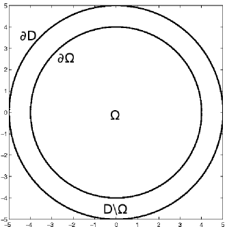
Figure 1: Test case for the Electrical Impedance Tomography. Circular inclusion $\Omega$ inside the circular body $\mathcal{D}$.

6.1 Numerical assessment of the goal-oriented estimator

We consider the configuration in figure 1, where $\mathcal{D}\coloneqq\{(x,y)\ |\ x^{2}+y^{2}\leq\rho_{E}^{2}\}$ and $\Omega\coloneqq\{(x,y)\ |\ x^{2}+y^{2}\leq\rho_{I}^{2}\}$. The values for the physical parameters are $\rho_{E}=5$, $\rho_{I}=4$, $k_{E}=1$ and $k_{I}=10$. The boundary datum for the Neumann problem (5.1) reads as $g=\cos(M\vartheta)\ ,\ M=5$. Using a polar coordinate system $(\rho,\vartheta)$, we can compute the following analytical solution:

$$u_{\Omega,N}=\begin{cases}C_{0}J_{M}\left(-i\rho k_{I}^{-\frac{1}{2}}\right)\cos(M\vartheta)\ &,\ \rho\in[0,\rho_{I}]\\ \left[C_{1}J_{M}\left(-i\rho k_{E}^{-\frac{1}{2}}\right)+C_{2}Y_{M}\left(-i\rho k_{E}^{-\frac{1}{2}}\right)\right]\cos(M\vartheta)\ &,\ \rho\in(\rho_{I},\rho_{E}]\end{cases}$$

where $J_{M}(\cdot)$ and $Y_{M}(\cdot)$ respectively represent the first- and second-kind Bessel functions of order $M$. The constants $C_{0},\ldots,C_{2}$ are detailed in table 1.

Constant	$\mathbb{R}\text{e}[C_{i}]$	$\mathbb{I}\text{m}[C_{i}]$
$C_{0}$	$-6.3\cdot 10^{-9}$	$+40.39491005$
$C_{1}$	$+1.30145994$	$+0.325482825$
$C_{2}$	$+1.5\cdot 10^{-11}$	$-1.301459935$

Table 1: Constants for the analytical solution.

For the approximation of the state equations (5.5), we consider both $\mathbb{P}^{1}$ and $\mathbb{P}^{2}$ Lagrangian Finite Element functions. In figures 2A and 2B, we present a comparison between the analytical error due to the discretization and the corresponding estimates arising from the complementary energy principle (Section 5.3.1) under uniform mesh refinements. We remark that using $\mathbb{P}^{1}$ Finite Elements, the estimated convergence rate is nearly $1$, whereas using $\mathbb{P}^{2}$ basis functions for the Finite Element space leads to a convergence rate slightly lower than $2$.

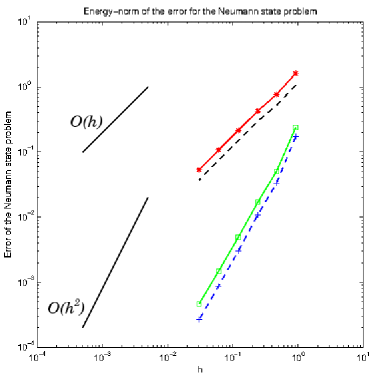
(A) Neumann problem.

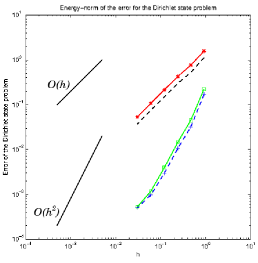
(B) Dirichlet problem.

Figure 2: Comparison of the convergence rates with respect to the mesh size $h$ for the (A) Neumann and (B) Dirichlet state equations. Analytical errors using $\mathbb{P}^{1}$ (black dash) and $\mathbb{P}^{2}$ (blue cross) Lagrangian Finite Element functions; error estimates based on the complementary energy principle using $\mathbb{P}^{1}$ (red star) and $\mathbb{P}^{2}$ (green square) Lagrangian Finite Element functions.

In order to construct the estimator for the error in the shape gradient, first we approximate equation (2.8) using $\mathbb{P}^{1}\times\mathbb{P}^{1}$ Lagrangian Finite Element functions. For the discretization of the adjoint equations (5.11), we use the same Finite Element space as for the state problems, whereas the dual fluxes in equations (5.20) and (5.24) are approximated using Raviart-Thomas Finite Element functions. In particular, we choose the space of $RT_{0}$ (respectively $RT_{1}$) functions when the state and adjoint equations are solved using $\mathbb{P}^{1}$ (respectively $\mathbb{P}^{2}$) Finite Elements.

In figure 3, we present the convergence history of the discretization error in the shape gradient, the error in the Quantity of Interest arising from its linearization and the corresponding complementary energy estimates provided in (5.10) using both $\mathbb{P}^{1}$ (Fig. 3A) and $\mathbb{P}^{2}$ (Fig. 3B) Finite Element functions. In both figure 3A and figure 3B, we remark that the error in the linearized Quantity of Interest is very similar to the one in the shape gradient. This confirms that the linearization error introduced in (3.5) is negligible with respect to the discretization error due to the Finite Element approximation and the estimator constructed from the linearized Quantity of Interest provides reliable information on the error in the shape gradient itself.
Figure 3A shows the evolution of the error in the Quantity of Interest with respect to the number of Degrees of Freedom of the problem under uniform mesh refinements. The error estimator shows an evolution which is analogous to the one of the analytical error in the shape gradient, thus we verify that an upper bound for the error in the Quantity of Interest is derived.

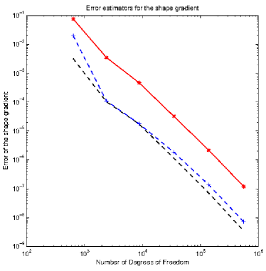
(A) $\mathbb{P}^{1}$ Finite Element.

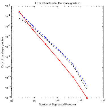
(B) $\mathbb{P}^{2}$ Finite Element.

Figure 3: Comparison of the convergence rates with respect to the number of Degrees of Freedom for the error in the Quantity of Interest using (A) $\mathbb{P}^{1}$ and (B) $\mathbb{P}^{2}$ Lagrangian Finite Element functions. Analytical error in the shape gradient (black dash); error in the linearized Quantity of Interest (blue cross); error estimator for the Quantity of Interest using the complementary energy principle (red star).

Nevertheless, when dealing with $\mathbb{P}^{2}$ Lagrangian Finite Element functions (Fig. 3B), the resulting error estimator for the Quantity of Interest underestimates the error in the shape gradient. This phenomenon may be caused by the error due to the approximation of the geometry that has not been accounted for in this work. As a matter of fact, in [28] Morin et al. observe that increasing the accuracy of the PDE approximation is useless if the expected geometrical error is higher than the one due to the discretization of the state problem. For this reason, in the following simulations, we stick to low-order Finite Element approximations ($\mathbb{P}^{1}-RT_{0}$) since using higher-order elements would prevent from getting a certified upper bound of the error in the shape gradient which is crucial for the application of the Certified Descent Algorithm.

6.2 1-mesh and 2-mesh reconstruction strategies

We may now apply the CDA to identify the unknown inclusion $\Omega$ inside the circular domain $\mathcal{D}$ using one boundary measurement. The initial inclusion is a circle of radius $\rho_{ini}=2$ and the associated computational mesh counting $472$ triangles is displayed in figure 4A.
It is well-known in the literature (cf. [4]) that using the same computational domain for both solving the state problem and computing a descent direction may lead to poor optimized shapes. In figures 4B and 4C we present the computational domains obtained using respectively a 1-mesh strategy to compute both the solutions $u_{\Omega,i}^{h}$’s and the descent direction $\theta^{h}$ and a 2-mesh approach in which the state equations are solved on a fine mesh whereas $\theta^{h}$ is computed on a coarser domain. A comparison of the reconstructed interfaces after $24$ and $25$ iterations is reported in figure 4D and as expected we observe that the 1-mesh algorithm provides a poor approximation of the inclusion whereas the 2-mesh strategy is able to precisely retrieve the boundary along which the conductivity $k_{\Omega}$ is discontinuous. Figures 4E and 4F confirm what was already observed by zooming on the local behavior of the interfaces and highlighting the oscillatory nature of the 1-mesh reconstruction.

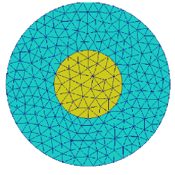
(A) $472$ elements.

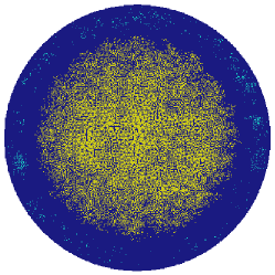
(B) $178047$ elements.

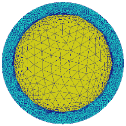
(C) $66833$ elements.

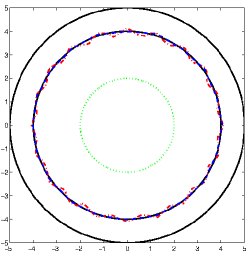
(D) Reconstructed interface.

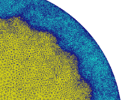
(E) 1-mesh interface.

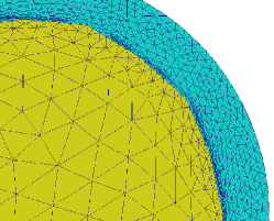
(F) 2-mesh interface.

Figure 4: Comparison of 1-mesh and 2-mesh reconstruction strategies. (A) Initial mesh. (B) Final mesh using 1-mesh strategy. (C) Final mesh using 2-mesh strategy. (D) Initial configuration (dotted green), target inclusion (solid black) and reconstructed interfaces using 1-mesh (dot-dashed red) and 2-mesh (dashed blue) strategies. (E) Zoom of the reconstructed interface using 1-mesh strategy. (F) Zoom of the reconstructed interface using 2-mesh strategy.

In figure 5A, we report the evolution of the objective functional with respect to the number of iterations using the two discussed approaches. It is straightforward to observe that the CDA identifies a genuine descent direction at each iteration, generating a sequence of minimizing shapes such that the objective functional $J(\Omega)$ is monotonically decreasing. Moreover, the error estimate in the shape gradient is also used to construct a guaranteed stopping criterion for the overall optimization strategy which automatically ends when $|\langle d_{h}J(\Omega),\theta^{h}\rangle|+\overline{E}<\texttt{tol}$ for an a priori set tolerance. Even though both versions of the algorithm generate shapes for which the functional is monotonically decreasing, only the 2-mesh strategy is able to precisely identify the target inclusion. For this reason, in the following sections we will focus only on the 2-mesh approach.

Besides the theoretical improvement of the Boundary Variation Algorithm discussed so far, an advantage of the CDA lies in the possibility of using relatively coarse meshes to identify certified descent directions. In figure 5B we observe that the number of Degrees of Freedom remains small until the reconstructed interface approaches the real inclusion, that is coarse meshes prove to be reliable during the initial iterations of the algorithm. Thus, another important feature of the Certified Descent Algorithm is the ability of certifying the reliability of coarse meshes for the identification of genuine descent directions for a shape functional, reducing the overall computational effort of the algorithm coupled with the a posteriori estimators during the initial phase of computation.

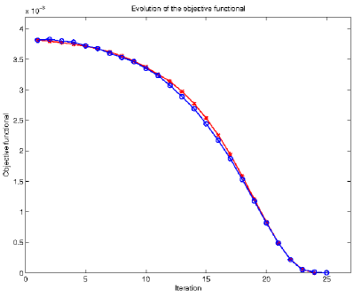
(A) Objective functional.

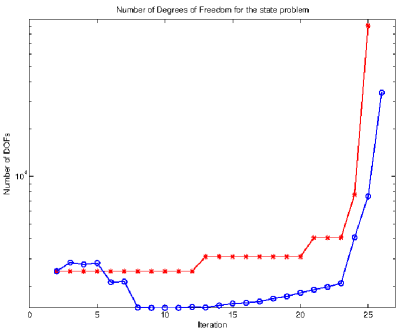
(B) Number of Degrees of Freedom.

Figure 5: Comparison of 1-mesh (red star) and 2-mesh (blue circle) reconstruction strategies. (A) Evolution of the objective functional. (B) Number of Degrees of Freedom.

6.3 A more involved test case

In the previous section, we applied the Certified Descent Algorithm to a simple test case and we were able to retrieve a precise description of the interface $\partial\Omega$. This was mainly due to the fact that the inclusion $\Omega$ was located near the external boundary $\partial\mathcal{D}$ where the measurements are performed. In this section, we consider a more involved test case: on the one hand, we break the symmetry of the problem by considering the initial and target configurations in figure 6A; on the other hand, we highlight the difficulties of precisely identifying the boundary of an inclusion when its position is far away from $\partial\mathcal{D}$.

As observed in the previous section, the evolution of the objective functional is monotonically decreasing (Fig. 6B - red curve), meaning a genuine descent direction is identified at each iteration of the optimization procedure. The final value of the approximated objective functional is $\mathcal{O}(10^{-4})$, in agreement with the zero value in the analytical optimal configuration of the inclusion.
Moreover, the evolution of the number of Degrees of Freedom (Fig. 6C - red curve) shows that coarse meshes prove to be reliable during initial iterations. The size of the problem remains small for several successive iterations but after few tens of iterations the CDA performs multiple mesh refinements in order to identify a genuine descent direction. This results in a high number of Degrees of Freedom which rapidly increases when approaching the configuration for which the criterion $|\langle d_{h}J(\Omega),\theta^{h}\rangle|+\overline{E}$ fulfills a given tolerance $\texttt{tol}=5\cdot 10^{-8}$.

In figure 6A, we observe that the part of the interface closest to $\partial\mathcal{D}$ is well identified using the Certified Descent Algorithm with one boundary measurement. Nevertheless when moving away from the external boundary, the precision of the reconstructed interface decreases and the algorithm is not able to precisely identify the whole inclusion. The uncertainty of the reconstruction in the central region of $\mathcal{D}$ is mainly due to the ill-posedness of the inverse problem. As a matter of fact, state problems (5.1) and (5.2) are elliptic equations thus the effect of the boundary conditions becomes less and less important moving away from $\partial\mathcal{D}$.

The case of multiple boundary measurements

A strategy to improve the quality of the reconstruction via the CDA relies on the use of several boundary measurements to retrieve a better approximation of the inclusion in a smaller number of iterations. The procedure to construct the set of boundary conditions to be used by the CDA is detailed in next section. Here, we present the outcome of the Certified Descent Algorithm using ten measurements for the test case featuring the circular domain $\mathcal{D}\coloneqq\{(x,y)\ |\ x^{2}+y^{2}\leq 25\}$ with the inclusion represented by the solid black line in figure 6A. We observe that using several boundary measurements the algorithm has access to more information to better identify the interface of the inclusion. First of all, the blue curve in figure 6A confirms the ability of the CDA to exactly identify the inclusion near the boundary $\partial\mathcal{D}$ and it highlights some minor improvements in the reconstruction of the interface with respect to the test case in red featuring one measurement (cf. the upper and lower parts of the ellipse). Nevertheless, the result is still degraded when moving towards the center of the domain. A possible workaround to this issue and to the low resolution of the reconstruction in the center of the computational domain is proposed by Ammari et al. in [5], where a hybrid imaging method arising from the coupling of electromagnetic tomography with acoustic waves is described.
The observed phenomenon is due to the well-known ill-posedness of the problem. Though considering several measurements improve the overall outcome of the algorithm, the final result is far from being satisfactory. Nevertheless, these limitations are related to the nature of the problem and we cannot expect gradient-based strategies to successfully overcome this issue. These remarks are confirmed by figure 6C. As a matter of fact, the number of Degrees of Freedom rapidly increases in both test cases, reaching $10^{5}$ and making the certification procedure unfeasible. Besides the improvement in the reconstructed interface, the use of several measurements is responsible for reducing the number of iterations required by the CDA to identify the inclusion (Fig. 6B). Moreover we remark that the tolerance that the quantity $|\langle d_{h}J(\Omega),\theta^{h}\rangle|+\overline{E}$ has to fulfill in this case drops to $\texttt{tol}=10^{-6}$, that is finer results are obtained in a smaller number of iterations and using lower precision in the case of multiple boundary measurements.

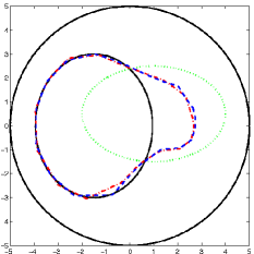
(A) Reconstructed interface.

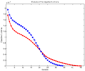
(B) Objective functional.

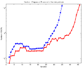
(C) Degrees of Freedom.

Figure 6: Certified Descent Algorithm using one measurement (red stars) and ten measurements (blue circles). (A) Initial configuration (dotted green), target inclusion (solid black) and reconstructed interface (dot-dashed red and dashed blue). (B) Evolution of the objective functional. (C) Number of Degrees of Freedom.

Sensitivity of the CDA to different initializations

It is well-known in the literature that gradient-based strategies are local, that is they are able to identify only local minima. Thus, a key aspect for the success of the optimization procedure is represented by the initialization of the unknown variable. For shape optimization problems, this reduces to the choice of the initial shape. In figure 7, we present three different initializations for the inclusion $\Omega$ and the corresponding final interfaces reconstructed by the Certified Descent Algorithm. The three test cases confirm the ability of the method to correctly retrieve the portion of the inclusion close to $\partial\mathcal{D}$ whereas the regions in the center of the domain suffer from a degraded reconstruction. Concerning the objective functional, the final values obtained using the proposed initializations are comparable (Fig. 8A), as the rapidly exploding number of Degrees of Freedom (Fig. 8B) which testifies again the ill-posedness of the inverse problem.

Remark 6.1.

In the literature concerning inverse problems, a key issue when discussing a new method is represented by its robustness to noise and data perturbations. It is straightforward to observe that the construction of the sets of boundary data $(g,U_{D})$ introduced at the beginning of this section is responsible for an additional contribution to the error. As previously observed, in order to retrieve reliable information to optimize the objective functional the Certified Descent Algorithm requires an extremely high precision after few tens of iterations. In real-world applications, this results to be completely unfeasible since the additional information arising from the high precision would be lost due to the noisy nature of the boundary data. Hence, for the purpose of this work we neglect the contribution of the uncertainty due to the measurements. An interesting extension of the current CDA may focus on the role of the error on the boundary measurements: in particular, an additional criterion may be integrated into the method in order to stop the algorithm if the error on the solutions of the state problems is smaller than the error on the data, that is if the effect of data fluctuations becomes predominant in the certification procedure.

(A) Initialization (I).

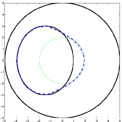
(B) Initialization (II).

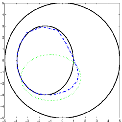
(C) Initialization (III).

Figure 7: Certified Descent Algorithm using multiple measurements for different initial configurations. Initial configuration (dotted green), target inclusion (solid black) and reconstructed interface (dashed blue).

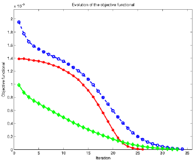
(A) Objective functional.

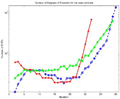
(B) Number of Degrees of Freedom.

Figure 8: Certified Descent Algorithm using multiple measurements for initial guess (I) blue circles; (II) red stars; (III) green diamonds. (A) Evolution of the objective functional. (B) Number of Degrees of Freedom.

6.4 The case of multiple boundary measurements

In [38], the authors prove that from an analytical point of view, one measurement is sufficient to uniquely reconstruct the inclusion within the Calderón’s problem. Other analytical results on this topic are presented in [1]. Nevertheless, from a numerical point of view, it is known that multiple measurements are required to have a correct approximation of the Electrical Impedance Tomography identification problem. In this section, we present several tests of the previously described algorithm using multiple boundary measurements. In particular, we consider $D=10$ measurements such that $\forall j=0,\ldots,D-1$

$$g_{j}(x,y)=(x+a_{j}y)^{b_{j}}a_{j}^{c_{j}}\quad,\quad a_{j}=1+0.1j\quad,\quad b_{j}=\frac{j+1}{2}\quad,\quad c_{j}=j-2\left\lfloor\frac{j}{2}\right\rfloor$$

and we use them to test the following cases:

1. one inclusion in a square domain (Fig. 9A-9C);

2. two inclusions in a circular domain (Fig. 9D-9F);

3. two inclusions in a square domain (Fig. 9G-9I).

First, we present a simulation in which the body is the square $\mathcal{D}\coloneqq[-4,4]^{2}$ featuring a single polygonal inclusion (Fig. 9C). Then, we propose two cases with multiple inclusions (Fig. 9F and 9I): in both simulations, we assume that the number of inclusions is known a priori and equals $2$ and that the conductivity $k_{\Omega}$ has only two values, one inside the inclusions and one for the background.

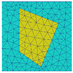
(A) $194$ elements.

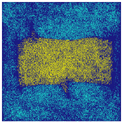
(B) $132040$ elements.

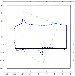
(C) Reconstructed interface.

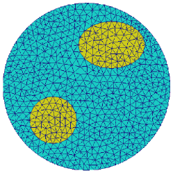
(D) $939$ elements.

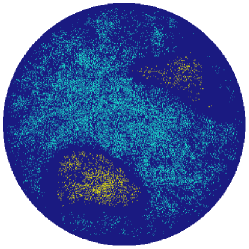
(E) $428251$ elements.

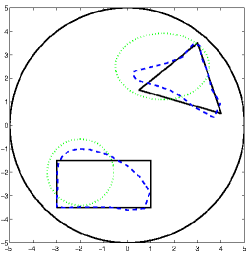
(F) Reconstructed interface.

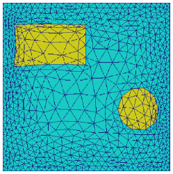
(G) $1616$ elements.

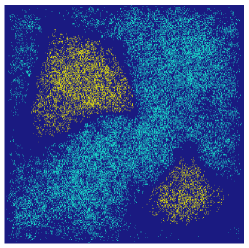
(H) $475744$ elements.

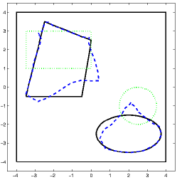
(I) Reconstructed interface.

Figure 9: Certified Descent Algorithm using multiple measurements: test cases (i)-(iii). Left: Initial mesh. Center: Final mesh. Right: Initial configuration (dotted green), target inclusion (solid black) and reconstructed interface (dashed blue).

As expected, the use of multiple measurements provides sufficient information to reconstruct the target interfaces near the boundary $\partial\mathcal{D}$ (Fig. 9C, 9F and 9I). On the contrary, the identification of the inner interfaces appears more difficult and with a less precise outcome. This phenomenon is due to the severe ill-posedness of the problem and the diffusive nature of the state equations is responsible for the loss of the information in the center of $\mathcal{D}$, even when using several measurements. In particular, we remark that the final interface in figure 9C still presents two kinks from the initial configuration: this is mainly due to the aforementioned phenomenon and may be bypassed by choosing a regularizing scalar product. However, this approach would lead to a global smoothing of the reconstructed interface, including a loss of information about the potential sharp physical corners of the polygonal inclusion.

As previously remarked, figure 10A confirms the monotonically decreasing behavior of the objective functional with respect to the iterations of the algorithm. Moreover, the quantitative information associated with the estimator of the error in the shape gradient allows to derive a reliable stopping criterion for the optimization procedure which results to be fully-automatic.
Eventually, coarse meshes are proved to be reliable for the computation during the initial iterations when the guessed position and shape of the inclusion is very unlikely to be precise. Within this context, even few Degrees of Freedom provide enough information to identify a genuine descent direction for the objective functional which we later certify using the discussed goal-oriented procedure. Thus, the same meshes may be used for several iterations increasing the number of Degrees of Freedom only when the descent direction is no more validated (Fig. 10B).
Both the inability of the method to reconstruct the interface far from the external boundary and the rapidly increasing number of Degrees of Freedom required to certify the descent direction clearly testifies the limitations of classical gradient-based approaches when dealing with the problem of Electrical Impedance Tomography. The ill-posedness of the problem is confirmed by the fact that after few tens of iterations, we are unable to identify a genuine descent direction at a small computational cost since the number of Degrees of Freedom required by the certification procedure rapidly reaches $10^{5}$. Nevertheless, the main novelty of the Certified Descent Algorithm - that is its certification procedure - provides us an heuristic criterion to stop the optimization routine when the number of Degrees of Freedom tends to explode, being the improvement of the solution negligible with respect to the huge precision the computation would require.

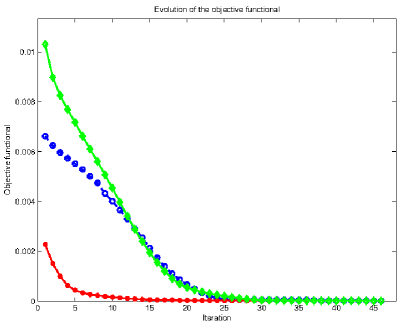
(A) Objective functional.

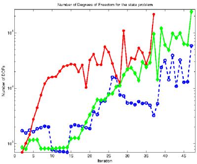
(B) Number of Degrees of Freedom.

Figure 10: Certified Descent Algorithm using multiple measurements: test case (i) blue circles; (ii) red stars; (iii) green diamonds. (A) Evolution of the objective functional. (B) Number of Degrees of Freedom.

7 Conclusion

In this work, we coupled classical shape optimization techniques with a goal-oriented error estimator for the shape gradient. A guaranteed bound for the error in the shape gradient has been derived by means of a certified a posteriori estimator.
On the one hand, introducing an a posteriori estimator for the error in the shape gradient provides quantitative information to define a reliable stopping criterion for the overall optimization procedure. Coupling this approach with the 2-mesh shape optimization strategy introduced in [4] results in the novel Certified Descent Algorithm. The CDA is a fully-automatic procedure for certified shape optimization: a validation of the method is presented by means of several test cases for the well-known inverse identification problem of Electrical Impedance Tomography. Another important feature of this method is the ability of identifying a certified descent direction at each iteration thus leading to a monotonically decreasing evolution of the objective functional.

Even though the CDA is able to make coarse meshes reliable to identify a genuine descent direction for the objective functional during the initial iterations, the overall computational cost tends to remain high. As a matter of fact, the major drawback of the described procedure is the necessity of solving the dual flux problems to derive a fully-computable upper bound of the error in the shape gradient. Hence, the Certified Descent Algorithm may result in higher computing times than the Boundary Variation Algorithm applied on fine meshes.

Ongoing research focuses on improving the a posteriori estimates for the discretization error in the shape gradient. Promising results are expected by the development of error estimators that only involve the computation of local quantities. Within this framework, accounting for anisotropic mesh adaptation [31] may lead to discretizations with a lower number of Degrees of Freedom and a better approximation of the physical problem.
Future investigations will focus on the application of the Certified Descent Algorithm to other challenging problems, such as the shape optimization of elastic structures.

References

- [1] L. Afraites, M. Dambrine, and D. Kateb. Shape methods for the transmission problem with a single measurement. Numer. Func. Anal. Opt., 28(5-6):519–551, 2007.
- [2] L. Afraites, M. Dambrine, and D. Kateb. On second order shape optimization methods for electrical impedance tomography. SIAM J. Control Optim., 47(3):1556–1590, 2008.
- [3] F. Alauzet, B. Mohammadi, and O. Pironneau. Mesh adaptivity and optimal shape design for aerospace. In G. Buttazzo and A. Frediani, editors, Variational Analysis and Aerospace Engineering: Mathematical Challenges for Aerospace Design, Springer Optimization and Its Applications, pages 323–337. Springer US, 2012.
- [4] G. Allaire and O. Pantz. Structural optimization with FreeFem++. Struct. Multidisc. Optim., 32(3):173–181, 2006.
- [5] H. Ammari, E. Bossy, J. Garnier, and L. Seppecher. Acousto-electromagnetic tomography. SIAM J. Appl. Math., 72(5):1592–1617, 2012.
- [6] H. Azegami, S. Kaizu, M. Shimoda, and E. Katamine. Irregularity of shape optimization problems and an improvement technique. In S. Hernandez and C. Brebbia, editors, Computer Aided Optimization Design of Structures V, pages 309–326. Computational Mechanics Publications, 1997.
- [7] N. Banichuk, F.-J. Barthold, A. Falk, and E. Stein. Mesh refinement for shape optimization. Struct. Optim., 9:46–51, 1995.
- [8] L. Borcea. Electrical impedance tomography. Inverse Prob., 18(6):R99, 2002.
- [9] A. Calderón. On an inverse boundary value problem. In Seminar on Numerical Analysis and its Applications to Continuum Physics (Rio de Janeiro 1980), pages 65–73. Soc. Brasil. Mat., 1980.
- [10] A. Carpio and M.-L. Rapún. Hybrid topological derivative and gradient-based methods for electrical impedance tomography. Inverse Problems, 28(9):095010, 22, 2012.
- [11] J. Céa. Conception optimale ou identification de formes, calcul rapide de la dérivée directionnelle de la fonction coût. ESAIM: Mathematical Modelling and Numerical Analysis, 20(3):371–402, 1986.
- [12] M. Cheney, D. Isaacson, and J. Newell. Electrical impedance tomography. SIAM Rev., 41:85–101, 1999.
- [13] E. Chung, T. Chan, and X.-C. Tai. Electrical impedance tomography using level set representation and total variational regularization. J. Comput. Phys., 205(1):357–372, 2005.
- [14] M. Delfour and J.-P. Zolésio. Shapes and geometries: analysis, differential calculus, and optimization. SIAM, Philadelphia, USA, 2001.
- [15] G. Dogǎn, P. Morin, R. Nochetto, and M. Verani. Discrete gradient flows for shape optimization and applications. Comput. Methods Appl. Mech. Engrg., 196(37–40):3898 – 3914, 2007. Special Issue Honoring the 80th Birthday of Professor Ivo Babuška.
- [16] K. Eppler and H. Harbrecht. A regularized Newton method in electrical impedance tomography using shape Hessian information. Control Cybernet., 34(1):203–225, 2005.
- [17] L. Formaggia, S. Micheletti, and S. Perotto. Anisotropic mesh adaption in computational fluid dynamics: application to the advection-diffusion-reaction and the Stokes problems. Appl. Numer. Math., 51(4):511–533, 2004.
- [18] T. Grätsch and K.-J. Bathe. Goal-oriented error estimation in the analysis of fluid flows with structural interactions. Comput. Methods Appl. Mech. Engrg., 195:5673–5684, 2006.
- [19] F. Hecht. New development in FreeFem++. J. Numer. Math., 20(3-4):251–265, 2012.
- [20] M. Hintermüller and A. Laurain. Electrical impedance tomography: from topology to shape. Control Cybern., 37(4):913–933, 2008.
- [21] M. Hintermüller, A. Laurain, and A. A. Novotny. Second-order topological expansion for electrical impedance tomography. Adv. Comput. Math., 36(2):235–265, 2012.
- [22] R. Hiptmair, A. Paganini, and S. Sargheini. Comparison of approximate shape gradients. BIT Numerical Mathematics, pages 1–27, 2014.
- [23] D. Holder. Electrical Impedance Tomography: Methods, History and Applications. Series in Medical Physics and Biomedical Engineering. CRC Press, 2004.
- [24] B. Jin and P. Maass. An analysis of electrical impedance tomography with applications to Tikhonov regularization. ESAIM Control Optim. Calc. Var., 18(4):1027–1048, 2012.
- [25] N. Kikuchi, K. Chung, T. Torigaki, and J. Taylor. Adaptive Finite Element Methods for shape optimization of linearly elastic structures. Comput. Method Appl. Mech. Eng., 57:67–89, 1986.
- [26] R. Kohn and M. Vogelius. Relaxation of a variational method for impedance computed tomography. Comm. Pure Appl. Math., 40(6):745–777, 1987.
- [27] A. Laurain and K. Sturm. Distributed shape derivative via averaged adjoint method and applications. M2AN Math. Model. Numer. Anal., 2015. to appear.
- [28] P. Morin, R. Nochetto, M. Pauletti, and M. Verani. Adaptive finite element method for shape optimization. ESAIM: Control Optim. Calc. Var., 18:1122–1149, 2012.
- [29] J. Oden and S. Prudhomme. Goal-oriented error estimation and adaptivity for the Finite Element Method. Comput. Math. Appl., 41(5-6):735 – 756, 2001.
- [30] O. Pantz. Sensibilité de l’équation de la chaleur aux sauts de conductivité. C. R. Acad. Sci. Paris, Ser. I(341):333–337, 2005.
- [31] G. Porta, S. Perotto, and F. Ballio. Anisotropic mesh adaptation driven by a recovery-based error estimator for shallow water flow modeling. Int. J. Numer. Meth. Fl., 70(3):269–299, 2012.
- [32] S. Prudhomme, J. Oden, T. Westermann, J. Bass, and M. Botkin. Practical methods for a posteriori error estimation in engineering applications. Internat. J. Numer. Methods Engrg., 56(8):1193–1224, 2003.
- [33] S. Repin. A posteriori error estimation for variational problems with uniformly convex functionals. Math. Comput., 69(230):481–500, 2000.
- [34] J. Roche. Adaptive Newton-like method for shape optimization. Control Cybern., 34(1):363–377, 2005.
- [35] M. Rüter, T. Gerasimov, and E. Stein. Goal-oriented explicit residual-type error estimates in XFEM. Comput. Mech., 52(2):361–376, 2013.
- [36] A. Schleupen, K. Maute, and E. Ramm. Adaptive FE-procedures in shape optimization. Struct. Multidisc. Optim., 19:282–302, 2000.
- [37] J. Sokołowski and J. Zolésio. Introduction to shape optimization: shape sensitivity analysis. Springer-Verlag, 1992.
- [38] J. Sylvester and G. Uhlmann. A global uniqueness theorem for an inverse boundary value problem. Ann. Math., 125:153–169, 1987.
- [39] T. Vejchodský. Complementary error bounds for elliptic systems and applications. Appl. Math. Comput., 219(13):7194 – 7205, 2013.
- [40] A. Wexler, B. Fry, and M. R. Neuman. Impedance-computed tomography algorithm and system. Appl. Opt., 24(23):3985–3992, 1985.