Abstract Graph Machine

Abstract

An Abstract Graph Machine(AGM) is an abstract model for distributed memory parallel stabilizing graph algorithms. A stabilizing algorithm starts from a particular initial state and goes through series of different state changes until it converges. The AGM adds work dependency to the stabilizing algorithm. The work is processed within the processing function. All processes in the system execute the same processing function. Before feeding work into the processing function, work is ordered using a strict weak ordering relation. The strict weak ordering relation divides work into equivalence classes, hence work within a single equivalence class can be processed in parallel, but work in different equivalence classes must be executed in the order they appear in equivalence classes. The paper presents the AGM model, semantics and AGM models for several existing distributed memory parallel graph algorithms.

1 Introduction

Graphs are ubiquitous data structures. Many real-world relations are formulated as graphs and graph algorithms are used to derive various characteristics related to those relations. Applications such as social networks, web search and scientific computing etc., use graph algorithms to derive useful information about graphs. As for many other data, graph relations are also growing so that they cannot be fit into a graph data structure in a single process. Those graphs need to be distributed among several computing resources and must be processed in parallel.

Designing, implementing and analyzing distributed memory parallel algorithms is inherently a difficult task due to several reasons: 1. distributed memory parallel algorithms depend on the data distribution used, 2. designing and implementing proper mutual exclusion and locking methods for distributed memory systems is hard, 3. graphs are irregular in memory access pattern. Therefore, the performance of graph algorithms is not predictable as in for other regular algorithms, 4. due to irregularity, graph algorithms heavily depend on the underlying run-time and the architecture.

To provide better solutions to above challenges, abstractions that help to understand the nature of distributed memory parallel graph algorithms are important. Developing such abstractions is difficult, due to the discrepancy between the solution approaches used in those distributed memory parallel graph algorithms. For example, Dijkstra’s Single Source Shortest Path [4] algorithm starts from a given source vertex and spread its search through neighbors, but Borůvka’s Minimum Spanning Tree [12] algorithm rely on set operations (disjoint union) to calculate the Minimum Spanning Tree (MST). While Borůvka’s Minimum Spanning Tree (MST) uses set operations in its solution, the Dijkstra’s Single Source Shortest Path (SSSP) algorithm relies on priority based ordering of distances of neighbors to calculate the SSSP. Therefore, the solution approach used in Dijkstra’s SSSP is different from the solution approach used in Borůvka’s MST algorithm.

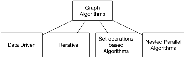
Figure 1: Graph algorithm classification based on their solution approach.

Based on the solution approach, we classify parallel graph algorithms into four categories (Figure 1): 1. Data-driven algorithms 2. Iterative algorithms 3. Set operations based algorithms 4. Nested parallel algorithms.

Data-driven algorithms associate a state to each vertex. At the start of the algorithm, vertex states are initialized to a specific value. The algorithm starts by changing the states of a subset of vertices. Whenever a vertex state is changed, its neighbors are notified. The state change is spread by notifying changes to neighbors. Towards to end of the algorithm, state changes will be reduced and states reach a fixed point. When there is no more state changes the algorithm terminates. An example of a data-driven algorithm is the Dijkstra’s SSSP.

As in data-driven algorithms, iterative algorithms also associate a state to a vertex, but instead of starting from a subset of vertices, iterative algorithms refine states associated with all vertices several iterations until all vertex states satisfy a defined condition. For example, in PageRank [13], the rank is calculated in iterations until rank values associated with all vertices are less than the defined error value. Shiloach-Vishkin Connected Components (CC) [14] is another example of an iterative algorithm.

Part of the set operations based algorithms, chase neighbors through edges, which is the standard action, should take place in a graph algorithm and rest of the algorithm rely on set operations. An example is Borůvka’s MST. Borůvka’s MST uses disjoint sets of components and relies on merging those components through set union operation to build the MST. Another example of a parallel graph algorithm that uses set operations is the Divide & Conquer Strongly Connected Components (DCSCC) [5]. In DCSCC, the vertex set is divided into two sets based on predecessor, successor reach-ability of a random vertex. Those two sets intersect to calculate the strongly connected component.

The nested parallel graph algorithms usually have an iterative or data-driven part. However, enclosing the iterative or data-driven section these algorithms have another iterative loop. An example for these kind of algorithms is the Parallel Betweeness Centrality [1] algorithm. Another example is All-Pairs Shortest Path algorithm.

Out of the algorithms discussed above, data-driven algorithms and iterative algorithms can be formulated as stabilizing algorithms, in which those algorithms start from a specific initial vertex state and goes through several state changes and converges. When all vertex states converged, the algorithm terminates. Further, those algorithms rely on standard graph operations rather than set operations. This paper proposes an abstract model for converging graph algorithms that only rely on graph operations.

The Abstract Graph Machine (AGM) is a mathematical abstraction for stabilizing graph algorithms. In AGM each vertex is associated with a state. States are changed by data propagating through edges. We call data propagating through edges work. The work is executed on a uniform function, i.e. same function is executed in every process. We call this function processing function. The processing function takes a unit of work as the parameter and may generate more work. Before processing, the work is ordered using a strict weak ordering relation. The strict weak ordering relation divides work into equivalence classes.

By dividing work into equivalence classes, the AGM controls the rate at which algorithm converges. When the amount of work in a single equivalence class is higher the amount of available data parallelism is also higher. However, when equivalence class is large the amount of unnecessary work (work that does not contribute to the final algorithm state) is also higher. The amount of work in a single equivalence class is decided by the nature of the strict weak ordering relation defined. The strict weak ordering relation also imposes an induced ordering on the equivalence classes. The equivalence classes are processed according to the induced order. Work within a single equivalence class can be processed in parallel but the processing of work in different equivalence classes is ordered.

The proposed abstraction provides a systematic way to study stabilizing graph algorithms. Using AGM, we can generalize existing data-driven graph algorithms and also derive new algorithms by composing orderings or by introducing new attributes into the definition of work. Further, AGM can be used for cost analysis of distributed memory parallel graph algorithms.

In general, we will assume graph $G=(V,E)$, where $V$ is the set of vertices and $E$ is the set of edges. The algorithm states are maintained in property maps and we assume graph and relevant property maps are distributed as a 1D distribution. After defining necessary prerequisites, we give the definition of an AGM in Section 2. Section 3, models data-driven graph algorithms in AGM. We discuss AGM applicability to non-data-driven algorithms in Section 4.

2 Abstract Graph Machine

In this section, we present the Abstract Graph Machine. First, we will define some of the terminologies that we will be using. Then, we will layout the structure of the AGM.

The main function that encapsulates the logic of a stabilizing algorithm is called the processing function. Parameters to the processing function is a single unit of work and we call it a $\mathit{workitem}$. The definition of the $\mathit{workitem}$ depends on the state/s in which algorithm is focused on and a $\mathit{workitem}$ must be indexed with a vertex or an edge. The set of all the $\mathit{workitems}$ that algorithm generates is the set $\mathit{WorkItem}$. When the processing function, processes a $\mathit{workitem}$, it may change the states associated with vertices. For example, in SSSP, the state is the distance from the source vertex and the processing function resembles the logic inside “relax”. For SSSP, a $\mathit{workitem}$ consists of a vertex and the distance associated to the vertex and $\mathit{WorkItem}\subseteq(V\times\mathbb{R}_{+}^{*})$.

An Abstract Graph Machine(AGM) consists of a definition of a $\mathit{WorkItem}$ set, an initial $\mathit{workitem}$ set, a set of states, a processing function and a strict weak ordering relation. In the following subsections, we discuss each of these parameters in detail.

2.1 The WorkItem Set

A $\mathit{workitem}$ is a tuple that has a vertex or an edge as of its first element. If the first element of a $\mathit{workitem}$ is a vertex, then we call that $\mathit{workitem}$ a vertex indexed $\mathit{workitem}$ and if the first element is an edge we call that $\mathit{workitem}$ an edge indexed $\mathit{workitem}$. The additional elements in the $\mathit{workitem}$, carry state data local to the vertex or an edge. For example, distance in a SSSP algorithm is an additional element in the “SSSP algorithm $\mathit{workitem}$”. In addition to vertex (or edge) and state data, a $\mathit{workitem}$ may carry ordering attributes. Ordering attributes are used when defining the strict weak ordering relation.

A $\mathit{workitem}$ is constructed and consumed within a processing function. The processing function, that constructs the $\mathit{workitem}$ may not reside in the same locality as the processing function, that consumes the $\mathit{workitem}$. In other words, $\mathit{workitems}$ can travel from one locality to another. A $\mathit{workitem}$ destination locality is decided based on the data distribution. For a 1D distributed graph and for a vertex indexed $\mathit{workitem}$, the destination locality is decided based on the ownership of the indexed vertex (i.e. the first element of the $\mathit{workitem}$). Details about data distribution is discussed in Section 2.2.

All the $\mathit{workitems}$ generated by an algorithm is the set $\mathit{WorkItem}$. $\mathit{WorkItem}$ is formally defined in Definition 1.

Definition 1

The $\mathit{WorkItem}$ is a set. For a given graph, G = (V, E), the $\mathit{WorkItem}\subseteq(V\times P_{0}\times P_{1}\dots\times P_{n})$ where each $P_{i}$ represents a state value or an ordering attribute value. A $\mathit{workitem}$ $\in\mathit{WorkItem}$ is represented as a tuple (e.g., $\mathit{workitem}$ = <$v,p_{0},p_{1}\dots,p_{n}$>  where $v\in V$ and each $p_{i}\in P_{i}$).

To access values in a $\mathit{workitem}$ tuple AGM uses bracket operator. e.g., if $w\in\mathit{WorkItem}$ and if $w$ = <$v,p_{0},p_{1}\dots,p_{n}$>then $w[0]$ = v and $w[1]$ = $p_{0}$ and $w[2]$ = $p_{1}$, etc.

2.2 Data Distribution

Data distribution is implicit in AGM and AGM always assumes that each vertex (or an edge) has a single owner node (process). Ownership of a $\mathit{workitem}$ is decided by the ownership of the indexed vertex (or edge) of the $\mathit{workitem}$. When a $\mathit{workitem}$ is being produced by a processing function it must be sent to its appropriate owner node for execution.

In addition, states are also distributed based on vertex (or edge) distribution. State value for a vertex (or edge) is only maintained at the owner.

2.3 States

AGM uses mappings to represent states. Each vertex or edge records a value algorithm is calculating. Collectively, all the values recorded against vertices or edges is treated as the state of the algorithm. States are read and updated by the processing function. In AGM terminology, accessing a state value associated with a vertex (or edge) “v” is denoted as “mapping_name(v)” (E.g :- distance(v), where distance is a mapping from vertex to distance from source in SSSP).

In addition to state mappings, processing functions access read-only graph properties. For example, “edge weight” is read as a read only property. In terms of syntax, AGM does not distinguish between a read-only property map and a state mapping. However, read-only graph properties such as “edge weight” are part of the graph definition.

States and read-only graph properties are only used within the processing function. Further, local updates to states are made atomically.

2.4 Processing Function

The processing function ($\pi$) takes a $\mathit{workitem}$ as an argument and may produce more $\mathit{workitems}$ (or 0) based on the logic defined inside the $\pi$. Mathematically, $\pi$ is declared as $\mathit{\pi}:\mathit{WorkItem}\longrightarrow\mathbb{P}(\mathit{WorkItem})$.

The processing function consists of a set of statements ( Definition 2). Each statement specifies, how the output $\mathit{workitem}$ (i.e., $w_{new}$) should be constructed (<constructor>), a condition based on input $\mathit{workitem}$ and/or states (<condition>) and an update to states (<state_update>). A statement is invoked if the condition evaluated to true. A statement may not generate new $\mathit{workitems}$ but only changes a state based on a condition. If a statement is only making changes to states based on input $\mathit{workitems}$, then it produces $w_{nil}$ $\mathit{workitem}$ as the output. The $\mathit{workitem}$ $w_{nil}$, is not treated as an active $\mathit{workitem}$; i.e., $w_{nil}$ is not ordered and also $w_{nil}$ is not fed to any of the processing functions for further processing.

Definition 2

$\mathit{\pi}:\mathit{WorkItem}\longrightarrow\mathbb{P}(\mathit{WorkItem})$

$$\mathit{\pi}(w)=\begin{cases}\{w_{new}|<constructor>,<state\_update>,\\ \;\;\;<condition>\}\\ \{w_{new}|<constructor>,<state\_update>,\\ \;\;\;<condition>\}\\ \dots\\ \{\}\;\;\;\;\mathit{else}\end{cases}$$

An algorithm starts by invoking processing function with the initial $\mathit{workitem}$ set. Output $\mathit{workitems}$ of the $\pi$ are ordered according to the strict weak ordering defined on $\mathit{workitems}$. Ordered $\mathit{workitems}$ are then again fed into the processing function. The interaction between $\pi$ and ordering is graphically depicted in Figure 2.

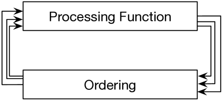
Figure 2: Interaction between ordering and the processing function in an AGM

2.5 Ordering

The AGM orders, output $\mathit{workitems}$ of the processing function using a strict weak ordering relation (denoted by $<_{\mathit{wis}}$). The strict weak ordering relation divides $\mathit{WorkItem}$ into equivalence classes based on the comparable relation ($<_{\mathit{wis}}$). The strict weak ordering relation must satisfy following properties;

1. For all $w\in\mathit{WorkItem}$ $w\nless_{\mathit{wis}}w$.

2. For all $w_{1},w_{2}\in\mathit{WorkItem}$ if $w_{1}<_{\mathit{wis}}w_{2}$ then $w_{2}\nless_{\mathit{wis}}w_{1}$.

3. For all $w_{1},w_{2},w_{3}\in\mathit{WorkItem}$ if $w_{1}<_{\mathit{wis}}w_{2}$ and $w_{2}<_{\mathit{wis}}w_{3}$ then $w_{1}<_{\mathit{wis}}w_{3}$.

4. For all $w_{1},w_{2},w_{3}\in\mathit{WorkItem}$ if $w_{1}$ not comparable with $w_{2}$ and $w_{2}$ not comparable with $w_{3}$ then $w_{1}$ is not comparable with $w_{3}$.

Properties 1 and 2 states that the strict weak ordering relation is not reflexive and antisymmetric. Property 3 denotes the transitivity of the “comparable $\mathit{workitems}$” and Property 4 states that transitivity is preserved among non-comparable elements in the $\mathit{workitem}$ set. These properties give rise to an equivalence (i.e. non-comparable $\mathit{workitems}$ belong to the same equivalence class) relation defined on $\mathit{workitem}$ set, hence partition the complete $\mathit{workitem}$ set. Since $\mathit{workitems}$ in different equivalence classes are comparable, the strict weak ordering relation defined on $\mathit{workitem}$ set induces an ordering on generated equivalence classes. In general, there are several ways to define the induced ordering relation (denoted $<_{\mathit{WIS}}$), for our work we stick to the definition given in  Definition 3.

Definition 3

$<_{\mathit{WIS}}$ is a binary relation defined on $\mathbb{P}(\mathit{WorkItem})$, such that if $W_{1},W_{2}\in\mathbb{P}(\mathit{WorkItem})$ then; $W_{1}\leq_{\mathit{WIS}}W_{2}\;iff\\ \;forall\;w_{1}\in W_{1}\;and\;forall\;w_{2}\in W_{2};w_{1}<_{\mathit{wis}}w_{2}$.

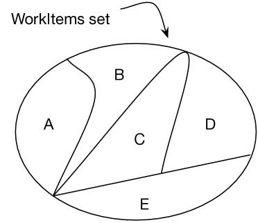
Figure 3: Partitioning $\mathit{workitems}$ based on strict weak order relation $<_{\mathit{wis}}$.

Figure 3, shows how $\mathit{WorkItem}$ is partitioned by the strict weak ordering relation $<_{\mathit{wis}}$. Sets A, B, C, D, E are mutually exclusive and $A\cup B\cup C\cup D\cup E=\mathit{WorkItem}$. Elements ($\mathit{workitems}$) in A are not comparable using $<_{\mathit{wis}}$, i.e. if $w_{1},w_{2}\in A$ then $w_{1}\nless_{\mathit{wis}}w_{2}$ nor $w_{2}\nless_{\mathit{wis}}w_{1}$. Same applies to other sets. Also, induced relation order partitions in a sequence. E.g., $B<_{\mathit{WIS}}D<_{\mathit{WIS}}A<_{\mathit{WIS}}E<_{\mathit{WIS}}C$; as per this example the smallest partition defined by $<_{\mathit{WIS}}$ is B.

2.6 The AGM

The AGM is formally defined in  Definition 4.

Definition 4

An Abstract Graph Machine(AGM) is a 6-tuple (G, $\mathit{WorkItem}$, Q, $\pi$, $<_{\mathit{wis}}$, S), where

1. G = (V, E) is the input graph,

2. $\textbf{$\mathit{WorkItem}$}\subseteq(V\times P_{0}\times P_{1}\dots\times P_{n})$ where each $P_{i}$ represents a state value or an ordering attribute,

3. Q - Set of states represented as property maps,

4. $\pi:\mathit{WorkItem}\longrightarrow\mathbb{P}(\mathit{WorkItem})$ is the processing function,

5. $<_{\mathit{wis}}$ - Strict weak ordering relation defined on $\mathit{workitems}$,

6. S ($\subseteq\mathit{WorkItem}$) - Initial $\mathit{workitem}$ set.

AGM execution starts with the initial $\mathit{workitem}$ set. The initial $\mathit{workitem}$ set is ordered according to the strict weak ordering relation. Then $\mathit{workitems}$ within the smallest equivalence class is fed to the $\pi$. If $\pi$ generates new $\mathit{workitems}$, they are again, separated into equivalence classes. The $\mathit{workitems}$ within a single equivalence class can execute $\pi$ in parallel. However, $\mathit{workitems}$ in two different equivalence classes must be ordered according to the induced relation (i.e. $<_{\mathit{WIS}}$). When executing $\mathit{workitems}$ in an equivalence class, it may generate new $\mathit{workitems}$ to the same equivalence class or to an equivalence class greater (as per $<_{\mathit{WIS}}$) than currently processing equivalence class. The AGM executes $\mathit{workitems}$ in next equivalence class, once it finished executing all the workitems in the current equivalence class. An AGM terminates when it executes all the $\mathit{workitems}$ in all the equivalence classes.

3 Data-driven Algorithms in AGM

A Data-driven algorithm starts from a subset of $\mathit{workitem}$ set, and generates more work as it progress. Towards to the end, the algorithm generates less work and comes to a termination when it does not generate more work. Most of the SSSP algorithms including Dijkstra’s Algorithm, $\Delta$-Stepping algorithm [11], KLA [9] SSSP algorithm are data-driven algorithms. Also, the Level Synchronous Breadth First Search [2], KLA Breadth First Search [9] and Push based Page Rank discussed in  [15] are also data-driven algorithms. In this section, we go through those data-driven algorithms and show the AGM formulation for each. Further, we present a data-driven Connected Components algorithm and an AGM formulation for that.

3.1 Single Source Shortest Path Algorithms

In this section, we go through several algorithms for SSSP application and show how they can be modeled using the Abstract Graph Machine defined in Definition 4.

In general, the $\mathit{workitem}$ set for SSSP application can be defined as $\mathit{WorkItem}^{sssp}\subseteq(V\times Distance)$, where Distance $\subseteq\mathbb{R}_{+}^{*}$. SSSP algorithms use distance as the output state and weight map as a read-only input mapping. The processing function for SSSP changes the distance state if input $\mathit{workitem}$’s distance is less than what is already stored in the distance map. Further, adjacent vertices of a given vertex are accessed through the neighbors function. (Declared as $neighbors:V\longrightarrow\mathbb{P}(V)$).

Interestingly, most of the SSSP algorithms share almost the same processing function. In general, the SSSP processing function ($\pi^{sssp}$) can be defined as follows;

Definition 5

$\pi^{sssp}:\mathit{WorkItem}^{sssp}\;\longrightarrow\mathit{WorkItem}^{sssp}$

$$\pi^{sssp}(w)=\begin{cases}\{w_{k}|<w_{k}[0]\in\mathit{neighbors}(w[0])\;\mathit{and}\\ \;\;\;w_{k}[1]\longleftarrow w[1]+\mathit{weight}(w[0],w_{k}[0])>\\ \;\;\;<distance(w[0])\longleftarrow w[1]>\\ \;\;\;<\mathit{if}\;w[1]<\mathit{distance}(w[0])>\}\\ \{\}\;\;\;\;\mathit{else}\end{cases}$$

The processing function definition given in Definition 5 is organized according to the general processing function definition given in 2. The processing function, $\pi$ has two statements. The first statement is executed only if $\mathit{workitem}$ distance is less than the value stored in the $distance$ state for the relevant vertex in $\mathit{workitem}$. Constructor of the first statement specifies how to construct a new $\mathit{workitem}$. In Definition 5, $w$ refers to currently processing $\mathit{workitem}$ and $w_{k}$ is the new $\mathit{workitem}$ that will be constructed. Further, the bracket operator is used to access $\mathit{workitem}$ elements (As discussed in Section 2.1). For $w\in\mathit{WorkItem}^{sssp}$, the term $w[0]$ refers to a vertex and $w[1]$ refers to the distance associated with the vertex referred by $w[0]$.

3.1.1 Dijkstra’s Algorithm

Dijkstra’s SSSP algorithm is the work efficient SSSP algorithm. Algorithm globally orders vertices by their associated distances and shortest distance vertices are processed first. In the following we define the ordering relation for Dijkstra’s algorithm and, we instantiate Dijkstra’s algorithm using an AGM.

Definition 6

$<_{\mathit{dj}}$ is a binary relation defined on $\mathit{WorkItem}^{sssp}$ as follows; Let $w_{1},w_{2}\in\mathit{WorkItem}^{sssp}$, then; $w_{1}<_{\mathit{dj}}w_{2}$ iff $w_{1}[1]<w_{2}[1]$

It can be proved that $<_{dj}$ is a strict weak ordering relation that satisfies constraints listed under Definition 6 (proof is omitted). AGM instantiation for Dijkstra’s algorithm is given in  Proposition 1.

Proposition 1

Dijkstra’s Algorithm is an instance of an AGM where;

1. $G=(V,E,weight)$ is the input graph,

2. $\mathit{WorkItem}$ = $\mathit{WorkItem}^{sssp}$,

3. Q = {distance} is the state mapping,

4. $\pi$ = $\pi^{sssp}$,

5. Strict weak ordering relation $<_{\mathit{wis}}$ = $<_{\mathit{dj}}$,

6. S = {<$v_{s}$, 0>} where $v_{s}\in V$ and $v_{s}$ is the source vertex.

3.1.2 $\Delta$-Stepping Algorithm

$\Delta$-Stepping [11] arrange vertex-distance pairs into distance ranges (buckets) of size $\Delta(\in\mathbb{N})$ and executes buckets in order. Within a bucket, vertex-distance pairs are not ordered, and can be executed in any order. Processing a bucket may produce extra work for the same bucket or for a successive bucket. The strict weak ordering relation for the $\Delta$-Stepping algorithm is given in Definition 7.

Definition 7

$<_{\Delta}$ is a binary relation defined on $\mathit{WorkItem}^{sssp}$ as follows; Let $w_{1},w_{2}\in\mathit{WorkItem}^{sssp}$, then;
$w_{1}<_{\Delta}w_{2}$ iff $\lfloor w_{1}[1]/\Delta\rfloor<\lfloor w_{2}[1]/\Delta\rfloor$

Instantiation of the $\Delta$-Stepping algorithm in AGM (given in Proposition 2) is same as in Proposition 1, except the strict weak ordering relation is $<_{\Delta}$ (= $<_{\mathit{wis}}$).

Proposition 2

$\Delta$-Stepping Algorithm is an instance of AGM where;

1. G = (V, E, weight) is the input graph

2. $\mathit{WorkItem}$ = $\mathit{WorkItem}^{sssp}$

3. Q = {distance} is the state mapping,

4. $\pi$ = $\pi^{sssp}$,

5. Strict weak ordering relation $<_{\mathit{wis}}$ = $<_{\Delta}$

6. S = {<$v_{s}$, 0>} where $v_{s}\in V$ and $v_{s}$ is the source vertex.

3.2 Breadth First Search (BFS) Algorithms

In this subsection, we present AGM models for two distributed memory parallel BFS algorithms. They are, level synchronous BFS and KLA BFS.

3.2.1 Level Synchronous BFS Algorithm

The level-synchronous breadth first search algorithm uses data structures to store the current and next vertex frontiers. Then the next container data is swapped with current after processing each level.

In the following we model level-synchronous BFS with the AGM. The level synchronous BFS order work by the level in the resulting BFS tree. Therefore, the ordering attribute, that we are interested in, is the level; hence we define $\mathit{WorkItem}^{bfs}\subseteq V\times Level$ where $Level\subseteq\mathbb{N}$.

The processing function for BFS is defined in Definition 8. The state of the BFS algorithm is maintained in a map ($vertex\_level:V\longrightarrow Level$) that store the level associated with each vertex. An infinite value (very large value) is associated to each vertex at the start of the algorithm. Then the infinite value is changed as the algorithm traverse through graph level by level.

Definition 8

$\pi^{bfs}:\mathit{WorkItem}^{bfs}\longrightarrow\mathbb{P}(\mathit{WorkItem}^{bfs})$

$$\pi^{bfs}(w)=\begin{cases}\{w_{k}|<w_{k}[0]\in neighbors(w[0])\;and\\ \;\;\;w_{k}[1]\longleftarrow w[1]+1>\\ \;\;\;<vertex\_level(w_{k}[0])\longleftarrow w[1]>\\ \;\;\;\;\;<(if\;vertex\_level(w_{k}[0])<\infty)>\}\\ \{\}\;\;\;\;else\end{cases}$$

The AGM is instantiated for level-synchronous BFS algorithm is given in Proposition 3.

Proposition 3

Level Synchronous BFS Algorithm is an instance of an AGM where;

1. G = (V, E) is the input graph,

2. $\mathit{WorkItem}$ = $\mathit{WorkItem}^{bfs}$,

3. Q = { vertex_level } is the state mapping,

4. $\pi$ = $\pi^{bfs}$,

5. The strict weak ordering relation $<_{\mathit{wis}}$ = $<_{bfs}$,

6. S = {<$v_{s}$, 0>} where $v_{s}\in V$ and $v_{s}$ is the source vertex.

3.2.2 KLA BFS Algorithm

The KLA BFS is similar to the level-synchronous BFS discussed above. Unlike in level-synchronous BFS, the KLA BFS processes $\mathit{workitems}$ asynchronously up to $k$ levels. In other words, $\mathit{workitems}$ are partitioned based on the value of $k$. The strict weak ordering relation for KLA is defined in  Definition 9.

Definition 9

$<_{kla}$ is a binary relation defined on $\mathit{WorkItem}^{bfs}$ as follows: Let $w_{1},w_{2}\in\mathit{WorkItem}^{bfs}$, then; $w_{1}<_{kla}w_{2}$ iff $\lfloor w_{1}[1]/k\rfloor<\lfloor w_{2}[1]/k\rfloor$

The AGM instantiation for KLA BFS is same as level synchronous BFS instantiation (Proposition 3), except the ordering relation is replaced with $<_{kla}$.

3.3 PageRank

PageRank(PR) [13] is a graph algorithm extensively used in web mining. Given a graph $G=(V,E)$, the PageRank, $PR(v)$ of a vertex $v$ is calculated using the formula given in Equation 1. The variable $\alpha$ represents the teleportation parameter. Function source returns the source vertex given an edge and functions in_edges and out_edges respectively return in and out edges of a given vertex.

$$PR(v)=(1-\alpha)+\alpha\sum_{e\in in\_edges(v)}\frac{PR(source(e))}{|out\_edges(source(e))|}$$ (1)

In PageRank, web pages are modeled as vertices and links between web pages are edges. The PageRank algorithm calculates a numeric weight for each page, which describes the importance of a web page.

Often PageRank algorithm is implemented as an iterative algorithm; i.e. algorithm iterate through all the vertices and calculates PageRank using the formula given in Equation 1. The algorithm continues to calculate rank values until the different between newly calculated value and the previous value is less than, a given error vale - $\epsilon$.

In the data-driven form of the algorithm, the PageRank of a vertex depends on the neighbours connected to the vertex using an in-edge. Whenever PageRank value of a neighbour connected through an in-edge changes, the PageRank of the current vertex must be re-calculated. A PageRank algorithm that uses this argument is also explained in [15]. The AGM formulation of the PageRank algorithm uses dependency between vertices (through in-edges) in terms of PageRank calculation to generate work.

In PageRank the final state we are interested in is the rank values of vertices. A straightforward way to model work for PageRank is to use vertex and rank value. One way to reduce the amount work is to order $\mathit{workitems}$ by the residual of a PageRank calculated for a vertex. (Residual based ordering is discussed in [15]). . Residual is the portion of the PageRank value that is being pushed through an out edge of a vertex.

Based on the residue value, the $\mathit{workitem}$ set for PageRank can be defined as $\mathit{WorkItem}^{pr}\subseteq(V\times\mathbb{R})$, where $\mathbb{R}$ is used to represent the residual value. The processing function for PageRank takes a $\mathit{workitem}$ ($\in\mathit{WorkItem}^{pr}$) and produces more $\mathit{workitems}$ if the difference between newly calculated PageRank value and previous PageRank value is greater than $\epsilon$. Further, the algorithm uses $rank$ mapping to store the calculated PageRank values. The processing function for PageRank is defined in Definition 10.

Definition 10

$\mathit{\pi^{pr}}:\mathit{WorkItem}^{pr}\longrightarrow\mathbb{P}(\mathit{WorkItem}^{pr})$

$$\mathit{\pi^{pr}}(w)=\begin{cases}\{w_{n}|<w_{n}[0]\in out\_neighbours(w[0])\;\&\\ \;\;\;w_{n}[1]\leftarrow\delta>\\ <pr_{new}\leftarrow PR(w[0])\;;\;\delta\leftarrow(pr_{new}-rank(w[0]))\\ \;\;\;;rank(w[0])\leftarrow pr_{new}>\\ <(\mathit{if}\;\delta>\epsilon)>\}\\ \{\}\;\;\;\;\mathit{else}\end{cases}$$

The PageRank algorithm converges quickly if we process higher residue $\mathit{workitems}$ first. Therefore, there are several possibilities to define ordering for PageRank: 1. do a strict comparison on residue value, 2. define strict weak ordering as in $\Delta$-Stepping 3. do not perform ordering at all. Each of the orderings creates a different size of equivalence class on PageRank $\mathit{workitems}$. However, for the formulation presented above, we define strict weak ordering ( Definition 11) only based on the comparison of residue values. Other orderings are also possible.

Definition 11

$<_{pr}$ is a binary relation defined on $\mathit{WorkItem}^{pr}$ as follows; Let $w_{1},w_{2}\in\mathit{WorkItem}^{pr}$, then;
$w_{1}<_{pr}w_{2}$ iff $w_{1}[1]>w_{2}[1]$.

The PageRank algorithm starts by assigning an initial rank to every vertex. Therefore the initial $\mathit{WorkItem}$ has a $\mathit{workitem}$ per each vertex and a associated residue value initialized to 0. More formally the initial $\mathit{WorkItem}$ $IW^{pr}=\{w|w[0]\in V\;and\;w[1]\leftarrow 0\}$.

With necessary parameters in hand we define the AGM formulation for PageRank algorithm in Proposition 4.

Proposition 4

PageRank Algorithm is an instance of an AGM where;

1. $G=(V,E)$ is the input graph,

2. $\mathit{WorkItem}$ = $\mathit{WorkItem}^{pr}$,

3. Q = {rank} is the state mapping,

4. $\pi$ = $\pi^{pr}$,

5. Strict weak ordering relation $<_{\mathit{wis}}$ = $<_{\mathit{pr}}$,

6. S = $IW^{pr}$

3.4 Connected Components Algorithm

For a given undirected graph, $G=(V,E)$, the connected component (CC) is a subgraph in which, any two vertices are connected through a path. A connected component can also be defined as a reachable relation. A vertex $v\;(\in V)$ is reachable to vertex $u\;(\in V)$ if and only if there is a path from $v$ to $u$.

In the literature, we find two main types of parallel connected component algorithms: 1. Shiloach-Vishkin’s $O(logn)$ based algorithms [14], 2. Search based algorithms [10]. Algorithms derived from Shiloach-Vishkin’s connected components are not data-driven algorithms. They are iterative algorithms and will be discussed in Section 4.0.1. In the following we discuss a search based connected component algorithm.

Search based algorithms mainly use Depth-first search (DFS), Breadth-first search (BFS) or a Chaotic search algorithm (See [10]). DFS based algorithms give little support to explore the available parallelism. Both BFS based algorithms and Chaotic search based algorithms have more opportunity to explore parallelism. To present the AGM formulation we will use a Chaotic search based algorithm.

A parallel search (Chaotic) based algorithm is given in Listing 1. Algorithm uses a property map (component) to record the component id of each vertex. Component map is the output state of the algorithm. Initially, the value of component id of a vertex is assigned to a very large number, then component map is updated when the function “CC” is invoked. The “VertexComponent” structure contains the vertex id and the component id for the vertex.

Algorithm 1 Search Based CC Algorithm

Input: Graph $G=(V,E)$

1:  Initialize() {

2:  for each vertex $v$ in $V$ do

3:     $component(v)\longleftarrow\infty$

4:  end for

5:  }

6:  

7:  CC(vc : VertexComponent) {

8:  $old\_component\longleftarrow component(vc.vertex)$

9:  if $vc.component<old\_component$ then

10:     $component(v)\longleftarrow vc.component$

11:     for each $v$ in adjacencies(vc.vertex) do

12:        CC(VertexComponent(v, vc.component))

13:     end for

14:  end if

15:  }

16:  

17:  Invoke() {

18:  Initialize()

19:  for each vertex $v$ in $V$ do

20:     CC(VertexComponent(v, v))

21:  end for

22:  }

We can develop several versions of the above algorithm. The algorithm in Listing 1 is a chaotic search algorithm. We also can develop the Dijkstra’s version and $\Delta$-Stepping version of the algorithm. In the following we model above algorithm using an AGM.

The $\mathit{workitems}$ for search based CC should include the distance and the component id (Since component id represents the state). Therefore, we define $\mathit{WorkItem}^{cc}\subseteq(V\times Component)$. In the definition the $Component\subseteq\mathbb{N}$. The processing function for search based CC is similar to SSSP processing function except it updates component id instead of the distance. Processing function for CC is given in Definition 12.

Definition 12

$\pi^{cc}:\mathit{WorkItem}^{cc}\longrightarrow\mathbb{P}(\mathit{WorkItem}^{cc})$

$$\pi^{cc}(w)=\begin{cases}\{w_{k}|<w_{k}[0]\in\mathit{neighbors}(w[0])\\ \;\;\;\;and\;w_{k}[1]\longleftarrow w[1]>\\ \;\;\;<component(w[0])\longleftarrow w[1]>\\ \;\;\;<\mathit{if}\;(w[1]<component(w[0])>\}\\ \\ \{\}\;\;\;\;\mathit{else}\end{cases}$$

We order $\mathit{workitems}$ by component id so that the smallest component ids are processed first. The order $\mathit{workitems}$ processed does not affect the correctness of the Algorithm 1. Therefore, more relaxed ordering can also be applied to CC AGM formulation. For simplicity we use the ordering based on component id. The strict weak ordering relation for CC is defined in Definition 13.

Definition 13

$<_{cc}$ is a binary relation defined on $\mathit{WorkItem}^{cc}$ as follows; Let $w_{1},w_{2}\in\mathit{WorkItem}^{cc}$, then;
$w_{1}<_{cc}w_{2}$ iff $w_{1}[1]<w_{2}[1]$.

In Proposition 5 we define the AGM for search based connected components.

Proposition 5

CC Algorithm is an instance of an AGM where;

1. $G=(V,E)$ is the input graph

2. $\mathit{WorkItem}$ = $\mathit{WorkItem}^{cc}$

3. Q = {components} is the state mapping,

4. $\pi$ = $\pi^{cc}$

5. Strict weak ordering relation $<_{\mathit{wis}}$ = $<_{cc}$

6. S = $\{w|w[0]\in V\;and\;w[1]=w[0]\}$.

4 AGM for Non-Data-driven
Algorithms

So far we modeled data-driven algorithms in AGM. A natural question to ask is whether AGM approach can be used to model other kinds of graph algorithms. The answer depends on the type of the graph algorithm we are focused on. For some types of graph algorithms AGM approach can be used with few modifications. Some other graph algorithms cannot be modeled using AGM due to the in-adequateness to express orderings using strict weak orderings and use set operations in those algorithms. In this section, we analyze the applicability of AGM to several non data driven algorithm types.

4.0.1 Iterative Algorithms

An iterative algorithm travels through all the vertices (or edges) until algorithm meets a specific state condition. Example algorithms are Iterative PageRank [8] and Shiloach-Vishkin Connected Components [14]. We use iterative PageRank as an example to dicuss the applicability of AGM to iterative algorithms, but discussion is general in which it applies to other iterative algorithms also.

Iterative PageRank iterate through all the vertices until all vertices reach a saturated PageRank value. PageRank value of a vertex is saturated if the difference between newly calculated PageRank value and the previous PageRank value is less than a defined error value. In the parallel iterative PageRank vertices in a single iteration are processed parallely and after each iteration algorithm checks whether the PageRank values has reached a saturation.

Vertices processed in parallel within a single iteration goes into a single equivalence class in the AGM formulation of the iterative PageRank. But vertices belonging to different iterations should be placed in different equivalence classes. Yet, after processing each equivalence class AGM must check whether PageRank has reached its saturation state.

The current, AGM formulation does not have fascility to check a condition before processing next equivalence class. The AGM can be augmented to check a condition after processing each equivalence class. Since equivalence classes are defined based on the iteration, a $\mathit{workitem}$ of an iterative algorithm must have the iteration number as a member and strict weak ordering must be defined in such a way, $\mathit{workitems}$ that has same iteration numbers are not comparable.

4.0.2 Divide & Conquer Algorithms

A Divide & Conquer algorithm recursively breaks down a problem into two or more sub problems, until they become sufficiently simple to solve. In a parallel Divide & Conquer algorithm divisions are conquered parallely. An example is Divide & Conquer Strongly Connected Components (DCSCC) [5]. The question is whether we can use AGM to express Divide & Conquer algorithms.

The answer is no, we cannot use AGM to express parallel Divide & Conquer algorithms. The main reason is that the strict weak ordering cannot be used to express the ordering in a Divide & Conquer algorithm in such a way it produces full available data parallelism. Ordering in divide & conqer algorithms is organized based on subset relationships of divisions. Therefore, the strict weak ordering is too strong to represent such ordering. In Appendix A we use DCSCC algorithm as an example to show that divide & conqer algorithm ordering cannot be expressed using a strict weak ordering. Rather, $\mathit{workitems}$ in DCSCC algorithm is ordered using a partial order (based on the subset relationship of divisions).

4.0.3 Algorithms with Nested Parallelism

Some algorithms show multiple levels of parallelism. Usually these algorithms have a visible data parallelism then a second level of task parallelism or data parallelism. Such nested parallel constructs are not easily transferrable to processing function so that it is amenable to execute in a distributed environment. We see these types of algorithms in applications such as Minimum Spanning Tree (MST) and Betweeness Centrality. In the following we use MST as an example and briefly analyze nested parallel algorithms in related to AGM.

A spanning tree, T of a graph G is a subgraph that includes all the vertices of G and is a tree. A minimum spanning tree (MST) of an undirected, connected, weighted graph G is a spanning tree that connects all the vertices with minimum weighted edges. There are 3 widely used algorithms to solve MST problem. They are 1. Prim’s Algorithm [3], 2. Kruskal Algorithm [3] and 3. Borůvka’s Algorithm [12].

Both Prim’s algorithm and Kruskal algorithm does not provide much data parallelism. However, Borůvka’s algorithm provides more parallelism and most of the existing parallel (and also distributed) implementations are based on Borůvka’s algorithm (See  [6]. [7]). Borůvka’s algorithm starts with a forest (i.e. each vertex is a component initially) and finds the minimum weight edge betwee two components. If algorithm finds a such edge, components are connected using the found edge.

To find the representative component set Borůvka’s algorithm uses disjoint union data structure. In a distributed setting calculating the representative set for a given source vertex and for a given target vertex of an edge can be performed in parallel. Therefore in addition to parallel processing of components algorithm also can process calculation of representative components for source vertex and target vertex in parallel.

The current AGM formulation does not have fascility to model nested levels of parallel work; i.e. work for parallel component processing and work for parallely calculate representative vertex sets for source and target of an edge. Another algorithm that shows the same behaviour is Parallel Betweeness Centrality [1] algorithm. Both algorithms generate parallel work in a fork-join like structure.

5 Conclusion

In this paper we presented Abstract Graph Machine (AGM), a mathematical model for distributed memory parallel graph algorithms that converges. The model formulate edge traversals as work and express an algorithm using a common function executed by every process in the system and an ordering that divides work into equivalence classes. We showed that existing data driven algorithms can be modeled using the AGM and also iterative algorithms. Algorithms that converge using set operations cannot be modeled in the AGM. We believe algorithms can be derived in such a way they can be modeled in the AGM.

Modeling algorithms using AGM generalizes existing algorithms, also model allows us to derive new variations of algorithms by changing the way algorithm order work. Ordering of an algorithm can be changed by either changing the average size of an equivalence class generated by the ordering or by introducing new ordering attributes. Further, in future we plan to use AGM model to build cost models for distributed memory parallel graph algorithms.

6 Acknowledgments

Authors (Thejaka) would like to thank Prabath Silva, for his valuable input on orderings in divided and conquer algorithms. I (Thejaka) thank Martina Barnas for many discussions about AGM algorithm abstractions and for her valuable feedback on this paper. Further, this material is based upon work supported by the National Science Foundation under Grant No. 1319520 and National Science Foundation under Grant No. 1111888.

Appendix A Strongly Connected
Components

Strongly Connected Component(SCC) is a subgraph of a directed graph where every vertex is reachable from every other vertex in the subgraph. The DCSCC algorithm for SCC selects a random vertex (pivot) and divides vertices set as vertices reachable from the pivot (descendents) and vertices that can reach the pivot (predecessors).  [5] proves that intersetion of predecessors and descendents is a strongly connected component containing the pivot.  [5] also proves that other SCC are either in predecessor set or descendent set or in the remainder ($=V-(predecessors\cup descendents)$). Then, DCSCC algorithm applies same procedure to descendents, predecessors and to remainder. Descendents (Let’s call this FWD set) and predecessors(BWD set) can be calculated in parallel. Then, DCSCC algorithm finds a strongly connected component (SCC) by calculating the set intersection of FWD and BWD. Afterwards, DCSCC algorithm divides vertex set into 3 segments. Segment1 = $FWD-SCC$, Segment2 = $BWD-SCC$ and Segment3 = $remainder$ (REM). Then each segment is processed in parallel. We can express the parallel execution of DCSCC in a tree as depicted in Figure 4.

Lemma 1

DCSCC algorithm cannot be modeled with an AGM.

Proof A.1.

Proof is by contradiction. Suppose DCSCC can be expressed using an AGM. Then, WorkItems in DCSCC can be ordered using a strict weak ordering relation $R$. R induces an equivalence relation and the induced relation partition work so that, work items in the same partition can be executed in parallel. Consider Figure 4. We should be able to execute work items in parallel as long as those work items does not relate to each other by a parent (including grand-parents) - child relationship. i.e. work items in $FWD^{1}-SCC^{1}$ and $FWD^{2}$ cannot be executed in parallel. Therefore $FWD^{1}-SCC^{1}$ and $FWD^{2}$ must belong to two different partitions in the induced equivalence relation (Partition 1 and Partition 2 in Figure 5). But we should be able to execute $FWD^{1}-SCC^{1}$ and $BWD^{1}-SCC^{1}$ in parallel as they dont relate to each other with a (grand)parent-child relationship. In other words, $FWD^{1}-SCC^{1}$ and $BWD^{1}-SCC^{1}$ belong to the same partition. Similarly $FWD^{2}$ and $BWD^{1}-SCC^{1}$ should belong to the same partition as they also can be executed in parallel. This shows that two partitions (partition belong to $FWD^{1}-SCC^{1}$ and partition belong to $FWD^{2}$) has an intersection (See Figure 5). This also shows that the induced relation does not divide work items into partitions $\implies$ The induced relation is not an equivalence relation $\implies$ R is not a strict weak ordering relation.

Therefore, our original assumption is wrong, i.e. there cannot be a strict weak ordering relation to divide work items in DCSCC and therefore we cannot express DCSCC in an AGM.

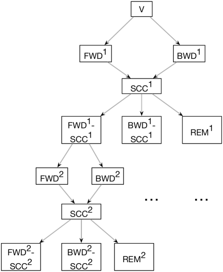
Figure 4: Parallel work in DCSCC algorithm.

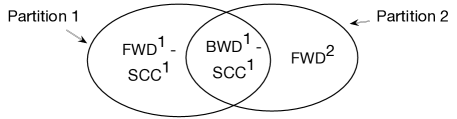
Figure 5: $BWD^{1}-SCC^{1}$ is the common intersection for two partitions.

References

- [1] D. A. Bader and K. Madduri. Parallel algorithms for evaluating centrality indices in real-world networks. In Parallel Processing, 2006. ICPP 2006. International Conference on, pages 539–550. IEEE, 2006.
- [2] A. Buluç and K. Madduri. Parallel breadth-first search on distributed memory systems. In Proceedings of 2011 International Conference for High Performance Computing, Networking, Storage and Analysis, page 65. ACM, 2011.
- [3] T. H. Cormen, C. Stein, R. L. Rivest, and C. E. Leiserson. Introduction to Algorithms. McGraw-Hill Higher Education, 2nd edition, 2001.
- [4] E. W. Dijkstra. A Note on Two Problems in Connexion With Graphs. Numerische mathematik, 1(1):269–271, 1959.
- [5] L. K. Fleischer, B. Hendrickson, and A. Pınar. On identifying strongly connected components in parallel. In Parallel and Distributed Processing, pages 505–511. Springer, 2000.
- [6] R. G. Gallager, P. A. Humblet, and P. M. Spira. A distributed algorithm for minimum-weight spanning trees. ACM Transactions on Programming Languages and systems (TOPLAS), 5(1):66–77, 1983.
- [7] J. A. Garay, S. Kutten, and D. Peleg. A sublinear time distributed algorithm for minimum-weight spanning trees. SIAM Journal on Computing, 27(1):302–316, 1998.
- [8] D. Gleich, L. Zhukov, and P. Berkhin. Fast parallel pagerank: A linear system approach. Yahoo! Research Technical Report YRL-2004-038, available via http://research. yahoo. com/publication/YRL-2004-038. pdf, 13:22, 2004.
- [9] Harshvardhan, A. Fidel, N. M. Amato, and L. Rauchwerger. KLA: A New Algorithmic Paradigm for Parallel Graph Computations. In Proc. 23rd Internat. Conf. on Parallel Architectures and Compilation, pages 27–38. ACM, 2014.
- [10] D. S. Hirschberg, A. K. Chandra, and D. V. Sarwate. Computing connected components on parallel computers. Communications of the ACM, 22(8):461–464, 1979.
- [11] U. Meyer and P. Sanders. -Stepping: A Parallelizable Shortest Path Algorithm. Journal of Algorithms, 49(1):114–152, 2003.
- [12] J. Nešetřil, E. Milková, and H. Nešetřilová. Otakar borůvka on minimum spanning tree problem translation of both the 1926 papers, comments, history. Discrete Mathematics, 233(1):3–36, 2001.
- [13] L. Page, S. Brin, R. Motwani, and T. Winograd. The pagerank citation ranking: bringing order to the web. 1999.
- [14] Y. Shiloach and U. Vishkin. An o (logn) parallel connectivity algorithm. Journal of Algorithms, 3(1):57–67, 1982.
- [15] J. J. Whang, A. Lenharth, I. S. Dhillon, and K. Pingali. Scalable data-driven pagerank: Algorithms, system issues, and lessons learned. In Euro-Par 2015: Parallel Processing, pages 438–450. Springer, 2015.