copyrightbox
DS-MLR: Exploiting Double Separability for Scaling up Distributed Multinomial Logistic Regression
Abstract
Scaling multinomial logistic regression to datasets with very large number of data points and classes is challenging. This is primarily because one needs to compute the log-partition function on every data point. This makes distributing the computation hard. In this paper, we present a distributed stochastic gradient descent based optimization method (DS-MLR) for scaling up multinomial logistic regression problems to massive scale datasets without hitting any storage constraints on the data and model parameters. Our algorithm exploits double-separability, an attractive property that allows us to achieve both data as well as model parallelism simultaneously. In addition, we introduce a non-blocking and asynchronous variant of our algorithm that avoids bulk-synchronization. We demonstrate the versatility of DS-MLR to various scenarios in data and model parallelism, through an extensive empirical study using several real-world datasets. In particular, we demonstrate the scalability of DS-MLR by solving an extreme multi-class classification problem on the Reddit dataset (159 GB data, 358 GB parameters) where, to the best of our knowledge, no other existing methods apply.
1 Introduction
In this paper, we focus on multinomial logistic regression (MLR) on massive datasets, in the presence of large number of data points and large number of classes. MLR is a method of choice for several real-world tasks such as Image Classification [18] and Video Recommendation [7]. Therefore, it has received significant research attention [9], [21]. The classic paradigm in distributed machine learning is to perform data partitioning, using, for instance, a map reduce style architecture where data is distributed across multiple slaves. In each iteration, the slaves gather the parameter vector from the master, compute gradients locally and transmit them back to the master. The L-BFGS optimization algorithm is typically used in the master to update the parameters after every iteration [15]. The main drawback of this strategy is that the model parameters need to be replicated on every machine. For a dimensional problem involving classes, this demands storage. In many cases, this is too large to fit on a single machine.
An orthogonal approach is to use model partitioning. Here again, a master slave architecture is used, but now, the data is replicated across each slave. The model parameters are partitioned and distributed to each machine. During each iteration, the model parameters on the individual machines are updated, and some auxiliary variables are computed and distributed to the other slaves, which use these variables in their parameter updates. See the Log-Concavity (LC) method [9] for an example of such a strategy. The main drawback of this approach, however, is that the data needs to be replicated on each machine, and consequently it is not applicable when the data is too large to fit on a single machine.
| Parameters | |||
| Fit | Do not Fit | ||
| Data | Fit | \pbox7cmL-BFGS, LC, | |
| DS-MLR | |||
& LC, DS-MLR Do not Fit \pbox7cmL-BFGS, DS-MLR DS-MLR
In contrast to the above approaches, we propose a reformulation of the objective function of multinomial logistic regression that allows us to simultaneously perform both data and model partitioning, thus enabling extreme classification at a massive scale with large number of data points and classes. We believe this is critical because, the growing acclaim of machine learning is witnessing several novel prediction tasks which not only involve humongous amounts of data, but also strive towards building more sophisticated models, demanding larger storage footprints. Table 1 presents a categorization of the various methods we discussed. DS-MLR can be applied in all the four scenarios. In Table 2, we compare their storage requirements in more detail. DS-MLR occupies the least amount of storage per worker. The main contributions of this work are:
-
1.
We develop DS-MLR, a novel distributed stochastic optimization algorithm that can partition both data as well as model parameters simultaneously across its workers.
-
2.
We develop a non-blocking and asynchronous variant (DS-MLR Async), which provides further speedups in the multi-core, multi-machine setting by interleaving the computation and communication phases during every iteration.
-
3.
We present an exhaustive empirical study spanning all the regimes of data and model parallelism, showing that DS-MLR readily applies in all cases. In particular, to demonstrate applicability in the scenario where both data and model do not fit on a single machine, we run DS-MLR on a large Reddit dataset with data and model parameters occupying 200 GB and 300 GB respectively.
| Storage per worker | Communication | ||
|---|---|---|---|
| Data | Parameters | ||
| L-BFGS | |||
| LC | |||
| DS-MLR | |||
The rest of the paper is organized as follows: Section 2 discusses related work. Section 3 formally introduces Multinomial Logistic Regression (MLR). Section 4 presents our reformulation (DS-MLR). In section 5, we discuss how our doubly separable objective function can be optimized in a distributed fashion and present synchronous and asynchronous algorithms for it. In section 6, we present rates of convergence for the synchronous version of DS-MLR. In section 7, we present empirical results running asynchronous DS-MLR covering all the regimes of data and model parallelism shown in Table 1. Finally, Section 9 concludes the paper.
2 Related Work
There has been a flurry of work in the past few years on developing distributed optimization algorithms for machine learning. Particularly, stochastic gradient descent based approaches have proven to be very fruitful since they make frequent parameter updates and converge much more rapidly [2]. Several algorithms for parallelizing SGD have been proposed in the past such as Hogwild [16], Parallel SGD [28], DSGD [8], FPSGD [26] and more recently, Parameter Server [12] and Petuum [20]. Although the importance of data and model parallelism has been recognized in Parameter Server and the Petuum framework [20], to the best of our knowledge this has not been exploited in their specific instantiations such as applications to multinomial logistic regression [19]. We believe this is because [19] does not reformulate the problem like the way DS-MLR does. Several problems in machine learning are not naturally well-suited for simultaneous data and model parallelism, and therefore such reformulations are essential in identifying a suitable structure. Moreover, the Parameter Server [12] is only a data parallel approach. This is because although the server maintains the model as a distributed key-value store, each worker maintains a working set of the entire model. This is in contrast with DS-MLR where at any given point of time, the model stays truly partitioned into mutually exclusive blocks across the workers.
Alternating direction method of multipliers (ADMM) [5] is another popular technique used to parallelize convex optimization problems. The key idea in ADMM is to reformulate the original optimization problem by introducing redundant linear constraints. This makes the new objective easily data parallel. However, ADMM suffers from a similar drawback as L-BFGS especially when applied to a multinomial logistic regression model. This is because the number of redundant constraints that need to be introduced are (# data points) (# classes) which is a major bottleneck to model parallelism. Moreover, the convergence rate of ADMM was found to be slow on multinomial logistic regression problems as discussed in [9].
Log-Concavity (LC) method [9] proposed a distributed model parallel approach to solve the multinomial logistic regression problem by linearizing the log-partition function based on its variational form [4]. However, because their formulation is only model parallel, the entire data has to be replicated across all the workers which is not practical for real world applications. Interestingly, we noticed that the objective function of the LC method can also be recovered from (5).
Our reformulation in DS-MLR exploits the doubly-separable structure in terms of global model parameters and some local auxiliary variables. Other doubly-separable methods also exist such as NOMAD [24] for matrix completion and RoBiRank [23] for latent collaborative retrieval. NOMAD [24] is a distributed-memory, asynchronous and decentralized algorithm and RoBiRank [23] is also a distributed-memory but synchronous algorithm. Parameter Server and HogWild [16] are asynchronous approaches. In Hogwild, parameter updates are executed in parallel using different threads under the assumption that any two serial updates are not likely to collide on the same data point when the data is sparse. DS-MLR does not make any such assumptions. It has both synchronous and asynchronous variants and the latter is in the spirit of NOMAD.
3 Multinomial Logistic Regression
Suppose we are provided training data which consists of data points where is a -dimensional feature vector and is a label associated with it; denotes the number of class labels. Let’s also define an indicator variable denoting the membership of data point to class . The probability that belongs to class is given by:
| (1) |
where denotes the parameter vector for each of the classes. Using the negative log-likelihood of (1) as a loss function, the objective function of MLR can be written as:
| (2) |
where regularizes the objective, and is a tradeoff parameter. Optimizing the above objective function (2) when the number of classes is large, is extremely challenging as computing the log partition function involves summing up over a large number of classes. In addition, it couples the class level parameters together, making it difficult to distribute computation. In this paper, we present an alternative formulation for MLR, to address this challenge.
4 Doubly-Separable Multinomial Logistic Regression (DS-MLR)
In this section, we present a reformulation of the MLR problem, which is closer in spirit to dual-decomposition methods [6]. We begin by first rewriting (2) as,
| (3) |
This can be expressed as a constrained optimization problem,
| (4) | ||||
where .
Observe that this resembles dual-decomposition methods of the form: s.t. , where and are convex functions. In our objective function (4), the decomposable functions are and respectively. Introducing Lagrange multipliers, , we obtain the equivalent unconstrained minimax problem [6],
| (5) |
It is known that dual-decomposition methods can reliably find a stationary point, therefore the solution obtained by our method is also globally optimal. We discuss the proof of convergence in section 6. The updates for the primal variables , and dual variable can be written as follows:
| (6) | ||||
| (7) | ||||
| (8) |
Here, and can be obtained by any black-box optimization procedure, while is updated via dual-ascent using a step-length . Intuitively, the dual-ascent update of penalizes any violation of the constraint in problem (4).
We now make the following interesting observations in these updates: Update for : When (7) is solved to optimality, admits an exact closed-form solution given by,
| (9) |
Update for : As a consequence of the above exact solution for , the dual-ascent update for is no longer needed, since the penalty is always zero during such a projection if is set to a constant equal to 1.
Update for : This is the only update that we need to handle numerically.
can be first written in this form,
| (10) |
where we denote for convenience and . The objective function is now doubly-separable [22] since,
| (11) |
where
| (12) |
Obtaining such a form for the objective function is key to achieving simultaneous data and model parallelism. It is worth pointing out that such an objective function can also be derived using the variational form for the log-partition function [4].
Stochastic Optimization: Minimizing involves computing the gradients of eqn (10) w.r.t. which is often computationally expensive. Instead, one can compute stochastic gradients [17] which are computationally cheaper than the exact gradient, and perform stochastic updates as follows:
| (13) |
where is the learning rate for . Being an unbiased stochastic gradient estimator, the standard convergence guarantees of SGD apply here [10].
Our formulation of DS-MLR in eqn (10) offers several key advantages:
-
1.
Observe that the objective function , now splits as summations over data points and classes. This means, each term in stochastic updates only depends one data point and one class . We exploit this to achieve simultaneous data and model parallelism.
-
2.
We are able to update the variational parameters in closed-form, avoiding noisy stochastic updates. This improves our overall convergence.
-
3.
Our formulation lends itself nicely to an asynchronous implementation. Section 5.2 describes this in more detail.
-
4.
Traditionally, dual-decomposition methods (e.g. ADMM) have been able to exploit distributed computing by solving separable sub-problems on multiple machines. Although this naturally led to data parallelism, it has not been clear so far how to separate the model parameters. For e.g. when applied to the MLR problem in the naive way, these methods introduce an additional storage (please refer to discussion in section 3.4 in [9]). In our reformulation (which bears a flavor of dual-decomposition methods), we demonstrate one way in which we can achieve both of these goals simultaneously. This is done by constraining the problem differently as shown in eqn (4) in our paper.
5 Distributing the Computation of DS-MLR
5.1 DS-MLR Sync
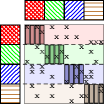
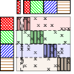
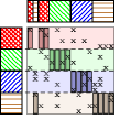
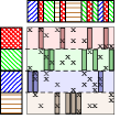
We first describe the distributed DS-MLR Synchronous algorithm in Algorithm 1. The data and parameters are distributed among the processors as illustrated in Figure 1 where the row-blocks and column-blocks represent data and weights on each local processor respectively. The algorithm proceeds by running iterations in parallel on each of the workers arranged in a ring network topology.

Each iteration consist of inner-epochs. During the first inner-epochs, each worker sends/receives its parameters to/from the adjacent machine and performs stochastic updates using the block of data and parameters that it owns. The second inner-epochs are used to pass around the to compute the exactly using (9).
5.2 DS-MLR Async
The performance of DS-MLR can be significantly improved by performing computation and communication in parallel. Based on this observation, we present an asynchronous version of DS-MLR. Due to the double-separable nature of our objective function (10), we can readily apply the NOMAD algorithm proposed in [24]. The entire DS-MLR Async algorithm is described in Algorithm 2.
The algorithm begins by distributing the data and parameters among workers in the same fashion as in the synchronous version. However, here we also maintain worker queues. Initially the parameters are distributed uniformly at random across the queues. The workers subsequently can run their updates in parallel as follows: each one pops a parameter out the queue, updates it stochastically and pushes it into the queue of the next worker. Simultaneously, each worker also records the partial sum (the local contribution of each worker towards the global normalization constant ) that is required for updating the variational parameters. This process repeats until updates have been made which is equivalent to saying that each worker has updated every parameter . Following this, the worker updates all its variational parameters exactly using the partial sums (9). For simplicity of explanation, we restricted Algorithm 2 to workers on a single-machine. However, in our actual implementation, we follow a Hybrid Architecture. This means that there are multiple threads running on a single machine in addition to multiple machines sharing the load across the network. Therefore, in this setting, each worker (thread) first passes around the parameter across all the threads on its machine. Once this is completed, the parameter is tossed onto the queue of the first thread on the next machine. Such a Hybrid Architecture does improve the experimental performance significantly since communication among threads locally within a machine is much less expensive than communication across threads which reside on different machines in the network.
6 Convergence
Although the semi-stochastic nature of DS-MLR makes it hard to directly apply the existing convergence results, under standard assumptions, it can be shown that it finds accurate solutions to the original objective in iterations.
Theorem 1
Suppose all for a constant . Let the step size in (13) decay at the rate of . Then, constant independent of and , such that
| (14) |
where is value of at the end of the iteration and denotes the data point. N, K, D, and P denote the number of data points, classes, dimensions and workers respectively.
It is worth noting that this rate of convergence is independent of the size of the problem. In particular, it is invariant to , the number of workers. Therefore, as more workers become available, the computational cost per iteration can be effectively distributed without sacrificing the overall convergence rate, up to the point where communication cost becomes dominant. Detailed proof is relegated to the Appendix A.
Our key idea in casting both algorithms as stochastic gradient descent methods is to demonstrate that although the update of is based on a stale value of arising from the delayed updates, such a delay still allows the error of the gradient of w.r.t to be bounded by , in Euclidean norm.
It should be noted that at this point our analysis and Theorem 1 applies only to the synchronous version of DS-MLR. The asynchronous version can be analyzed by upper-bounding the delay parameter and following proof techniques on the lines of [11] and [13].
7 Experiments
In our empirical study, we will focus on DS-MLR Async. We use a wide scale of real-world datasets of varying characteristics which is described in Table 3. Our experimental setup follows the same categorization we outline in Table 1.
| Dataset | # instances | # features | #classes | data (train + test) | parameters | sparsity (% nnz) | Methods that apply |
|---|---|---|---|---|---|---|---|
| CLEF | 10,000 | 80 | 63 | 9.6 MB + 988 KB | 40 KB | 100 | L-BFGS, LC, DS-MLR |
| NEWS20 | 11,260 | 53,975 | 20 | 21 MB + 14 MB | 9.79 MB | 0.21 | L-BFGS, LC, DS-MLR |
| LSHTC1-small | 4,463 | 51,033 | 1,139 | 11 MB + 4 MB | 465 MB | 0.29 | L-BFGS, LC, DS-MLR |
| LSHTC1-large | 93,805 | 347,256 | 12,294 | 258 MB + 98 MB | 34 GB | 0.049 | LC, DS-MLR |
| ODP | 1,084,404 | 422,712 | 105,034 | 3.8 GB + 1.8 GB | 355 GB | 0.0533 | LC, DS-MLR |
| YouTube8M-Video | 4,902,565 | 1,152 | 4,716 | 59 GB + 17 GB | 43 MB | 100 | L-BFGS, DS-MLR |
| Reddit-Small | 52,883,089 | 1,348,182 | 33,225 | 40 GB + 18 GB | 358 GB | 0.0036 | DS-MLR |
| Reddit-Full | 211,532,359 | 1,348,182 | 33,225 | 159 GB + 69 GB | 358 GB | 0.0036 | DS-MLR |
Hardware: All single-machine experiments were run on a cluster with the configuration of two 8-core Intel Xeon-E5 processors and 32 GB memory per node. For multi-machine multi-core, we used Intel vLab Knights Landing (KNL) cluster with node configuration of Intel Xeon Phi 7250 CPU (64 cores, 200GB memory), connected through Intel Omni-Path (OPA) Fabric. The asynchronous, non-blocking property of DS-MLR makes it ideal to be run on KNL, which is a many-core (68 core, 272 threads) architecture with massive FPLOPs, memory bandwidth, and large memory space (MCDRAM + DDR).
Implementation Details: We implemented our DS-MLR method in C++ using MPI for communication across nodes and Intel TBB for concurrent queues and multi-threading. To make the comparison fair, we re-implemented the LC [9] method in C++ and MPI using ALGLIB for the inner optimization. Finally, for the L-BFGS baseline, we used the TAO solver (from PETSc).
7.1 Data Fits and Model Fits
For this experiment, we compare DS-MLR, L-BFGS and the LC methods on small scale datasets CLEF, NEWS20, LSHTC1-small.
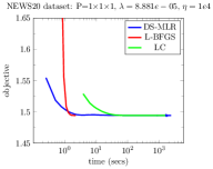
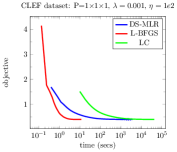
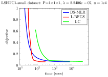
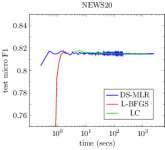
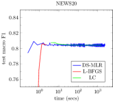
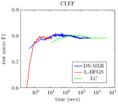
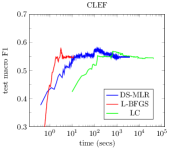
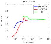
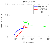
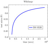
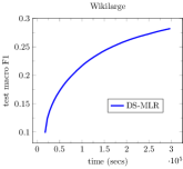
L-BFGS is a highly efficient second-order method that has a rapid convergence rate. Even when pitched against such a powerful second order method, DS-MLR performs considerably well in comparison. In fact, on some datasets such as NEWS20, DS-MLR is almost on par with L-BFGS in terms of decreasing the objective and also achieves a better f-score much more quickly. Figure 3 shows the progress of objective function as a function of time for DS-MLR, L-BFGS and LC on NEWS20, CLEF, LSHTC1-small datasets. The corresponding plots showing f-score vs time are available in Appendix C. However, L-BFGS loses its applicability when the number of parameters increases beyond what can fit on a single-machine.
DS-MLR consistently shows a faster decrease in objective value compared to LC on all three datasets: NEWS20, LSHTC1-small and CLEF. In fact, LC has a tendency to stall towards the end and progresses very slowly to the optimal objective value. In CLEF dataset, to reach an optimal value of 0.398, DS-MLR takes 1,262 secs while LC takes 21,003 secs. Similarly, in LSHTC1-small, to reach an optimal value of 0.065, DS-MLR takes 1,191 secs while LC takes 32,624 secs.
7.2 Data Fits and Model Does not Fit
For this experiment, we compare DS-MLR and LC on LSHTC1-large and ODP datasets.
LSHTC1-large: L-BFGS requires all its parameters to fit on one machine and is therefore not suited for model parallelism (even on modestly large datasets such as LSHTC1-large, 4.2 billion parameters need to be stored demanding 34GB). Thus, parallelizing L-BFGS would involve duplicating 34 GB of parameters across all its processors. We ran both DS-MLR and LC using 48 workers.
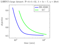
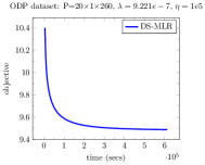
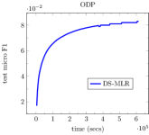
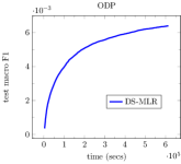
Figure 4 (left) shows how the objective function changes vs time for DS-MLR and LC. As can be seen, DS-MLR out performs LC by a wide-margin despite the advantage LC has by duplicating data across all its processors. ODP: We ran DS-MLR on the ODP dataset 111https://github.com/JohnLangford/vowpal_wabbit/tree/master/demo/recall_tree/odp which has a huge model parameter size of 355 GB. For this experiment we used 20 nodes 1 mpi task 260 threads. The progress in decreasing the objective function value is shown in Figure 4 (right). LC method being a second-order method has a very high per-iteration cost and it takes an enormous amount of time to finish even a single iteration.
7.3 Data Does not Fit and Model Fits
YouTube8M-Video: This dataset was created by pre-processing the publicly available dataset of youtube video embeddings 222https://research.google.com/youtube8m/ into a multi-class classification dataset consisting of 4,716 classes and 1,152 features. Since it was created from features derived from embeddings, it is a perfectly dense dataset.
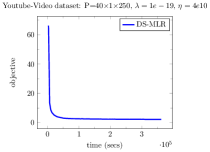
We used the configuration of 20 nodes 1 mpi tasks 260 threads to run DS-MLR on this dataset and we observed a fast convergence as shown in Figure 5. This is likely because DS-MLR being non-blocking and asynchronous in nature runs at its peak performance on a dense dataset like YouTube8M-Video, since the number of non-zeros in the data remains uniform across all its workers.
7.4 Data Does not Fit and Model Does not Fit
Reddit datasets: In this sub-section, we demonstrate the capability of DS-MLR to solve a multi-class classification problem of massive scale, using a bag-of-words dataset RedditFull created out of 1.7 billion reddit user comments spanning the period 2007-2015.
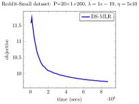
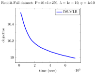
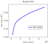
Our aim is to classify a particular reddit comment (data point) into a suitable sub-reddit (class). The data and model parameters occupy 200 GB and 300 GB respectively. Therefore, both L-BFGS and LC cannot be applied here. We also created a smaller subset of this dataset Reddit-Small by sub-sampling around 50 million data points. The result of running DS-MLR on these are shown in Figure 6. This experiment corresponds to the last scenario in Table 1 where simultaneous data and model parallelism is inevitable.
In Appendix B we study the predictive quality of DS-MLR and Appendix C has additional plots showing progress of f-score vs time.
8 Scaling behavior of DS-MLR
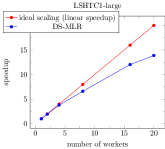
In Figure 7, we look at the speedup curves obtained on LSHTC1-large as the number of workers are varied as . The ideal speedup which corresponds to a linear speedup is denoted in red.
9 Conclusion
In this paper, we present a new stochastic optimization algorithm (DS-MLR) to solve multinomial logistic regression problems having large number of examples and classes, by a reformulation that makes it both data and model parallel simultaneously. As a result, DS-MLR can scale to arbitrarily large datasets where to the best of our knowledge, many of the existing distributed algorithms cannot be applied. Our algorithm is distributed, asynchronous, non-blocking and avoids any bulk-synchronization overheads. We provide empirical results showing DS-MLR applies to all regimes of distributed machine learning, especially the case where both data and model sizes exceed the memory capacity of a single machine. We show this on an extreme multi-class classification reddit dataset consisting of 200 GB data and 300 GB parameters respectively. In terms of future work, DS-MLR has several possible extensions such as extreme multi-label classification.
References
- [1] D. P. Bertsekas. Nonlinear programming. 1999.
- [2] L. Bottou. Large-scale machine learning with stochastic gradient descent. In Proceedings of COMPSTAT’2010. Springer, 2010.
- [3] L. Bottou and O. Bousquet. The tradeoffs of large-scale learning. Optimization for Machine Learning, page 351, 2011.
- [4] G. Bouchard. Efficient bounds for the softmax function, applications to inference in hybrid models. 2007.
- [5] S. Boyd, N. Parikh, E. Chu, B. Peleato, and J. Eckstein. Distributed optimization and statistical learning via the alternating direction method of multipliers. Foundations and Trends® in Machine Learning, 3(1):1–122, 2011.
- [6] S. Boyd and L. Vandenberghe. Convex Optimization. Cambridge University Press, Cambridge, England, 2004.
- [7] J. Davidson, B. Liebald, J. Liu, P. Nandy, T. Van Vleet, U. Gargi, S. Gupta, Y. He, M. Lambert, B. Livingston, et al. The youtube video recommendation system. In Proceedings of the fourth ACM conference on Recommender systems, pages 293–296. ACM, 2010.
- [8] R. Gemulla, E. Nijkamp, P. J. Haas, and Y. Sismanis. Large-scale matrix factorization with distributed stochastic gradient descent. ACM, 2011.
- [9] S. Gopal and Y. Yang. Distributed training of large-scale logistic models. In Proceedings of the 30th International Conference on Machine Learning (ICML-13), pages 289–297, 2013.
- [10] H. Kushner and G. G. Yin. Stochastic approximation and recursive algorithms and applications, volume 35. Springer Science & Business Media, 2003.
- [11] R. Leblond, F. Pedregosa, and S. Lacoste-Julien. Asaga: asynchronous parallel saga. arXiv preprint arXiv:1606.04809, 2016.
- [12] M. Li, L. Zhou, Z. Yang, A. Li, F. Xia, D. G. Andersen, and A. Smola. Parameter server for distributed machine learning. In Big Learning NIPS Workshop, 2013.
- [13] J. Liu, S. J. Wright, C. Ré, V. Bittorf, and S. Sridhar. An asynchronous parallel stochastic coordinate descent algorithm. The Journal of Machine Learning Research, 16(1):285–322, 2015.
- [14] A. Nedić and D. Bertsekas. Convergence rate of incremental subgradient algorithms. In Stochastic optimization: algorithms and applications, pages 223–264. Springer, 2001.
- [15] J. Nocedal and S. J. Wright. Numerical Optimization. Springer Series in Operations Research. Springer, 2nd edition, 2006.
- [16] B. Recht, C. Re, S. Wright, and F. Niu. Hogwild: A lock-free approach to parallelizing stochastic gradient descent. In Advances in Neural Information Processing Systems, pages 693–701, 2011.
- [17] H. E. Robbins and S. Monro. A stochastic approximation method. Annals of Mathematical Statistics, 22:400–407, 1951.
- [18] O. Russakovsky, J. Deng, H. Su, J. Krause, S. Satheesh, S. Ma, Z. Huang, A. Karpathy, A. Khosla, M. Bernstein, et al. Imagenet large scale visual recognition challenge. International Journal of Computer Vision, 115(3):211–252, 2015.
- [19] P. Xie, J. K. Kim, Y. Zhou, Q. Ho, A. Kumar, Y. Yu, and E. P. Xing. Distributed machine learning via sufficient factor broadcasting. CoRR, 2015.
- [20] E. P. Xing, Q. Ho, W. Dai, J. K. Kim, J. Wei, S. Lee, X. Zheng, P. Xie, A. Kumar, and Y. Yu. Petuum: a new platform for distributed machine learning on big data. Big Data, IEEE Transactions on, 2015.
- [21] I. E.-H. Yen, X. Huang, P. Ravikumar, K. Zhong, and I. Dhillon. Pd-sparse : A primal and dual sparse approach to extreme multiclass and multilabel classification. In Proceedings of The 33rd International Conference on Machine Learning, pages 3069–3077, 2016.
- [22] H. Yun. Doubly Separable Models. PhD thesis, Purdue University West Lafayette, 2014.
- [23] H. Yun, P. Raman, and S. Vishwanathan. Ranking via robust binary classification. In Advances in Neural Information Processing Systems, 2014.
- [24] H. Yun, H.-F. Yu, C.-J. Hsieh, S. Vishwanathan, and I. Dhillon. Nomad: Non-locking, stochastic multi-machine algorithm for asynchronous and decentralized matrix completion. 2013.
- [25] M. D. Zeiler. Adadelta: An adaptive learning rate method. CoRR, abs/1212.5701, 2012.
- [26] Y. Zhuang, Y.-C. Juan, and C.-J. Lin. A fast parallel stochastic gradient method for matrix factorization in shared memory systems. 2013.
- [27] M. Zinkevich, J. Langford, and A. J. Smola. Slow learners are fast. In Advances in Neural Information Processing Systems 22. 2009.
- [28] M. Zinkevich, M. Weimer, L. Li, and A. J. Smola. Parallelized stochastic gradient descent. In Advances in Neural Information Processing Systems, pages 2595–2603, 2010.
In the following sections, we provide a more detailed proof of convergence for our algorithm and also include additional plots from our empirical study.
Appendix A Rates of convergence
First the diameter of space can be bounded by a universal constant (independent of ) because we can always enforce that (ignoring log term). We also assume all are bounded in norm by some constant . We will write as a constant everywhere. They are not necessarily equal; in fact we may write and as . It just stands for some constant that is independent of and .
We index outer iteration by superscript and inner-epochs within each outer iteration by subscript . So , which we also denote as . We consider optimizing the objective
| (15) |
where . Clearly has a variational representation
| (16) |
where the optimal is attained at . So given , we can first compute the optimal , and then use it to compute the gradient of via the variational form (Danskin’s theorem [1]).
| (17) |
Here if is true, and 0 otherwise.
Due to the distributed setting, we are only able to update to their optimal value at the end of each epoch (i.e. based on ):
| (18) |
We are not able to compute the optimal for the latest when incremental gradient is performed through the whole dataset. Fortunately, since is updated in an epoch by a fixed (small) step size , it is conceivable that the computed from will not be too bad as a solution in (A) for , . In fact, if is order , then the following Lemma says the gradient computed from (17) using the out-of-date is also away from the true gradient at .
Lemma 2
Denote the approximate gradient of evaluated at based on as
| (19) |
where . Then .
Proof Unfolding the term from (18),
Therefore
So it suffices to upper bound the gradient of . Since and are bounded, is lower bounded by a positive universal constant333If one is really really meticulous and notes that which does involve , one should be appeased that is for any .. Now,
Using Lemma 2, we can now show that our algorithm achieves epoch complexity, with no dependency on , , or . In fact we just apply Nedic’s algorithm [14] and analysis on . However we need to adapt their proof a little because they assume the gradients are exact.
First we need to bound some quantities. because is bounded, and for numbers on a simplex with , we have . Without loss of generality, suppose is used for update at step . Then is subtracted by , where is Kroneker product and is a canonical vector. As long as , we can recursively apply Lemma 2 and derive bounds
| (20) | ||||
| (21) | ||||
| (22) |
for all . Now we run Nedic’s proof. Then for any
Telescoping over , we obtain that for all and :
Using the fact that is bounded by a universal constant, we further derive
Now use the standard step size of , we conclude
| (23) |
Note the proof has not used the convexity of in (A) at all. This is reasonable because it is “optimized out”.
Appendix B Rank Distribution
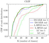
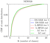
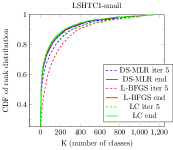
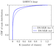
In this section, we plot the cumulation distribution of ranks of test labels. This is a proxy for the precision@k curve and gives a more closer indication of the predictive performance of a multinomial classification algorithm. In Figures 8 and 9, we plot the precision obtained after the first 5 iterations (denoted by dashed lines), and after the end of optimization (denoted by solid lines). As seen, DS-MLR performs competitively and in general tends to give a good accuracy within the first 5 iterations.
Appendix C Additional Plots
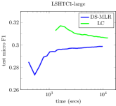
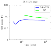
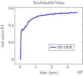
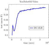
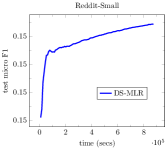
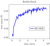
In this section, we show how the macro and micro f-score change as a function of time on the various datasets reported in Table 3.
