$SO(2)$-induced breathing patterns in multi-component Bose-Einstein condensates

Abstract

In this work, we employ the $SO(2)$-rotations of a two-component, one-, two- and three-dimensional nonlinear Schrödinger system at and near the Manakov limit, to construct vector solitons and vortex structures. This way, stable stationary dark-bright solitons and their higher-dimensional siblings are transformed into robust oscillatory dark-dark solitons (and generalizations thereof), with and without a harmonic confinement. By analogy to the one-dimensional case, vector higher-dimensional structures take the form of vortex-vortex states in two dimensions and, e.g., vortex ring-vortex ring ones in three dimensions. We consider the effects of unequal (self- and cross-) interaction strengths, where the $SO(2)$ symmetry is only approximately satisfied, showing the dark-dark soliton oscillation is generally robust. Similar features are found in higher dimensions too, although our case examples suggest that phenomena such as phase separation may contribute to the associated dynamics. These results, in connection with the experimental realization of one-dimensional variants of such states in optics and Bose-Einstein condensates (BECs), suggest the potential observation of the higher-dimensional bound states proposed herein.

I Introduction

One of the most paradigmatic models of multi-component system dynamics within integrable nonlinear systems and wave phenomena is the so-called Manakov model manakov ; intman1 . This is a vector variant of the famous nonlinear Schrödinger (NLS) equation sulem ; ablowitz ; siambook , featuring equal (nonlinear) interactions within a certain component and across the different ones. Vector solitons of this model have attracted considerable interest, both in the case of focusing ablowitz and defocusing siambook ; rip nonlinearities.

In the present setting, the case that will be of interest is that of the defocusing nonlinearity, as referred to in nonlinear optics; on the other hand, in the context of atomic Bose-Einstein condensates (BECs) stringari , this case corresponds to repulsive interatomic interactions, and is thus referred to as repulsive nonlinearity. In the original, one-dimensional (1D) Manakov system a particularly intriguing structure that is supported is the so-called dark-bright (DB) soliton. Here, the bright soliton component, which would not otherwise exist in the defocusing setting, arises because of an effective potential well created by the dark soliton through the inter-component interaction. In that light, DB solitons can be considered as “symbiotic” structures. The extensive study of such states christo ; vdbysk1 ; vddyuri ; ralak ; dbysk2 ; shepkiv ; parkshin , has stemmed in good measure from their potential applications in optics, where dark solitons were proposed to effectively act as adjustable waveguides for weak signals kivshar . In this field, the theoretical/analytical developments were (already a couple of decades ago) supplemented by experimental work in photorefractive media pioneering the observation of DB structures seg1 ; seg2 .

Our work is largely inspired by the setting of atomic condensates, where such structures have been explored in multiple recent experiments. The latter, were chiefly focusing on the dynamics of pseudo-spinor (two-component) atomic gases, featuring two hyperfine states of the same atom species, such as ⁸⁷Rb. Here, the early theoretical prediction of DB solitons buschanglin was – after a considerable hiatus – followed by the experimental realization by the Hamburg group hamburg . This, in turn, led to numerous further directions of explorations, many of which were pursued at Pullman pe1 ; pe2 ; pe3 ; pe4 ; pe5 ; azu . In particular, in Ref. hamburg , robust DB solitons were created by a phase-imprinting technique and their robust oscillations were probed in a quasi-1D parabolic trap. On the other hand, in subsequent experiments, different types of structures, including DB and dark-dark (DD) solitons pe1 ; pe2 ; pe3 ; pe4 ; pe5 , emerged spontaneously via instabilities in counterflow dynamical scenarios.

In the BEC setting, one of the significant advantages of the spinor gases is that, naturally, the coefficients of inter- and intra-component interactions are very close to being identical; in fact, the differences are not more than a few percent, which is important, e.g., in phase separation siambook ; stringari ; emergent . Hence, the model is naturally proximal (in as far as its nonlinearity coefficients are concerned) to the Manakov one. Remarkably, the Manakov case bears an additional symmetry under rotations, i.e., the model is invariant under the action of the $SU(2)$ Lie group. This invariance has been employed in order to generate unitary (in fact, chiefly orthogonal) rotations of states, such as the DB solitons. The resulting waveforms, produced even experimentally pe4 ; pe5 , are a particular form of DD solitons. Depending on the frequency (chemical potential, as we will refer to it below), the resulting evolution of the components can be intrinsically oscillatory i.e., breathing in their atomic density. While the transformation is exact only in the Manakov case, weak deviations from this integrable limit relevant to the atomic species appear to maintain such DD states as sufficiently robust nonlinear excitations in order for them to be experimentally observable.

In the present work, we extend the consideration of such states to higher dimensions. In particular, in section II, we revisit the mathematical framework of the $SU(2)$ and more specifically the $SO(2)$ group generator that produces the relevant invariance. For completeness, and also to make connections with earlier work, in section III.A we start with the 1D case by briefly discussing the DD soliton, stemming from the rotation of the DB one. We then examine the two-dimensional (2D) case, by considering vortex-bright solitons. The latter, involve a vortex in one component trapping a bright soliton in the other component kodyprl ; pola . These structures, are also known as “filled core vortices” (that were experimentally observed in Ref. anders ), “half-quantum vortices” tsubota ; adhikari or “baby Skyrmions” cooper , and their stability and dynamics, have been studied, respectively, in Refs. skryabin ; kodyprl and Refs. kodyprl ; tsubota . Rotating these in section III.B, we obtain (by analogy to the DD states) vortex-vortex structures with their constituent vortices rotating around one another. Finally, we turn to the three-dimensional (3D) setting, and examine the cases of vortex lines and vortex rings, which are the prototypical excitations therein siambook ; komineas . Once again, our starting point is the vortex-line, or vortex-ring in the first component, that traps a (line or ring, respectively) bright soliton in the second component. The rotation of such a stationary state allows us to capture a vector vortex-ring state with its own intrinsic vibrating dynamics, as we will illustrate in what follows in section III.C. Finally, in section IV, we summarize our findings and present a number of possibilities for future study.

II The model and analytical/computational setup

We start by presenting our model, as well as the analytical and computational setup. We consider the coupled defocusing NLS system written in dimensionless form siambook as

$$i\partial_{t}{\Phi_{-}} = -\frac{1}{2}\nabla^{2}\Phi_{-}+\left(g_{11}|\Phi_{-}|^{2}+g_{12}|\Phi_{+}|^{2}\right)\Phi_{-}+V(\mathbf{r})\,\Phi_{-},$$ (1a)

$$i\partial_{t}{\Phi_{+}} = -\frac{1}{2}\nabla^{2}\Phi_{+}+\left(g_{21}|\Phi_{-}|^{2}+g_{22}|\Phi_{+}|^{2}\right)\Phi_{+}+V(\mathbf{r})\,\Phi_{+},$$ (1b)

where $\nabla^{2}$ stands for the standard Laplace operator in the respective dimension of the problem, the interaction coefficients are $g_{jk}>0$ ($\forall j,k=1,2$), with $g_{21}\equiv g_{12}$, and the external potential $V(\mathbf{r})$ assumes the standard harmonic form of $V(\mathbf{r})=\frac{1}{2}\Omega^{2}|\mathbf{r}|^{2}$, with $|\mathbf{r}|^{2}=x^{2}+y^{2}+z^{2}$ and normalized trap strength $\Omega$ (note that in 1D, $\nabla^{2}=\partial_{x}^{2}$, $V=\frac{1}{2}\Omega^{2}x^{2}$, and so on). The fields (representing the macroscopic wavefunctions in BECs siambook ) $\Phi_{\pm}=\Phi_{\pm}(\mathbf{r},t)$ in Eqs. (1a)-(1b) are assumed to carry the dark (with “$-$” subscript) and bright (with “$+$” subscript) soliton components, respectively.

The starting point for our discussion below is the construction of stationary solutions. Such stationary solutions to Eqs. (1a) and (1b) with chemical potentials $\mu_{\pm}$ are found by employing the well-known ansatz,

$$\Phi_{\pm}(\mathbf{r},t)=\phi_{\pm}(\mathbf{r})\exp(-i\mu_{\pm}t),$$ (2)

where $\phi_{\pm}(\mathbf{r})$ stand for the steady states of the corresponding solitary waveforms. Then, Eqs. (1a)-(1b) reduce to the coupled system of stationary equations

$$\mu_{-}\phi_{-} = -\frac{1}{2}\nabla^{2}\phi_{-}+\left(g_{11}|\phi_{-}|^{2}+g_{12}|\phi_{+}|^{2}\right)\phi_{-}+V(\mathbf{r})\,\phi_{-},$$ (3a)

$$\mu_{+}\phi_{+} = -\frac{1}{2}\nabla^{2}\phi_{+}+\left(g_{12}|\phi_{-}|^{2}+g_{22}|\phi_{+}|^{2}\right)\phi_{+}+V(\mathbf{r})\,\phi_{+}.$$ (3b)

A key point in our analysis is that, as is well known (see, e.g., Ref. parkshin ), the Manakov model [cf. Eqs. (1) in 1D with $g_{ij}=1$ and without an external potential] is invariant under the action of the $SU(2)$ Lie-group. In fact, this result does not depend on the dimensionality of the system or the presence of an external potential (with the constraint that it should be the same for the two components), as long as $g_{ij}=1$. Indeed, let us first recall that a general matrix element of $SU(2)$ has the form

$$U=\left(\begin{array}[]{ccc}\alpha&-\bar{\beta}\\ \beta&\bar{\alpha}\end{array}\right),$$

where bar denotes complex conjugate, and complex constants $\alpha$ and $\beta$ are such that $|\alpha|^{2}+|\beta|^{2}=1$. Then, it can be shown that if the (pseudo-) spinor $(\Phi_{-},~{}\Phi_{+})^{T}$ is a solution of Eqs. (1), then,

$$\left(\begin{array}[]{ccc}\Phi_{-}^{\prime}\\ \Phi_{+}^{\prime}\end{array}\right)\equiv U\left(\begin{array}[]{ccc}\Phi_{-}\\ \Phi_{+}\end{array}\right)=\left(\begin{array}[]{ccc}\alpha\Phi_{-}-\bar{\beta}\Phi_{+}\\ \beta\Phi_{-}+\bar{\alpha}\Phi_{+}\end{array}\right),$$

is also a solution of Eqs. (1). In our considerations for what follows, we will focus on the special case of an $SO(2)$ rotation parametrized by an angle $\delta\in[0,2\pi)$ with a $2\times 2$ matrix representation

$$U\equiv R(\delta)=\begin{pmatrix}\cos{\delta}&-\sin{\delta}\\ \sin{\delta}&\cos{\delta}\end{pmatrix},$$ (4)

corresponding to the choice of $\alpha=\cos{\delta}$ and $\beta=\sin{\delta}$. Then, once stationary solutions in the form of Eq. (2) are identified, the rotation operator $R(\delta)$ given by Eq. (4) acts on $\mathbf{\Phi}=(\Phi_{-},\Phi_{+})^{T}$ as follows:

$$\mathbf{\Phi}\rightarrow\mathbf{\Phi^{\prime}}=R(\delta)\,\mathbf{\Phi}=\begin{pmatrix}\cos{\delta}\,\phi_{-}\exp(-i\mu_{-}t)-\sin{\delta}\,\phi_{+}\exp(-i\mu_{+}t)\\ \sin{\delta}\,\phi_{-}\exp(-i\mu_{-}t)+\cos{\delta}\,\phi_{+}\exp(-i\mu_{+}t)\end{pmatrix}.$$ (5)

It is now straightforward to determine the densities of the rotated fields $\Phi_{\pm}^{\prime}$, which read:

$$n_{-}^{\prime} \equiv |\Phi_{-}^{\prime}|^{2}=|\phi_{-}|^{2}\cos^{2}\delta+|\phi_{+}|^{2}\sin^{2}\delta-\sin(2\delta){\rm Re}\{\phi_{+}\bar{\phi}_{-}\exp[i\,\Delta\mu\,t]\},$$ (6a)

$$n_{+}^{\prime} \equiv |\Phi_{-}^{\prime}|^{2}=|\phi_{-}|^{2}\sin^{2}\delta+|\phi_{+}|^{2}\cos^{2}\delta+\sin(2\delta){\rm Re}\{\phi_{+}\bar{\phi}_{-}\exp[i\,\Delta\mu\,t)\},$$ (6b)

where $\Delta\mu=\mu_{-}-\mu_{+}$. The above equations indicate that the total density,

$$n^{\prime}=n_{-}^{\prime}+n_{+}^{\prime}=|\phi_{-}|^{2}+|\phi_{+}|^{2},$$ (7)

is time-independent (recall that $\phi_{\pm}$ depend only on $\mathbf{r}$), while the individual densities $n_{\pm}^{\prime}$ of the rotated states are periodic functions of time. In fact, the relevant angular frequency, which constitutes the internal beating frequency of the rotated structures, is $\omega=\Delta\mu$, while the period of internal vibrations is given by:

$$T=\frac{2\pi}{\Delta\mu}.$$ (8)

Our algorithm for the construction of the rotated (beating) dark-dark solitons and generalizations thereof in higher dimensions is described as follows. At first, we identify steady states $\phi_{\pm}$ to Eq. (3) using a Newton-Raphson method for a given set of chemical potentials $\mu_{\pm}$. This state will be of the dark-bright variety in 1D, of the vortex-bright in 2D, and of the vortex-line (VL)–bright (VLB) and vortex-ring (VR)–bright (VRB) in 3D. In the majority of the cases studied below, we consider two cases as far as the interaction coefficients are concerned (unless otherwise noted):

• $g_{ij}=1$, i.e., equal interaction coefficients, and

• unequal ones with $g_{11}=1.03$, $g_{12}=1$, and $g_{22}=0.97$.

We have used these values as “typical” ones appearing in the context of ⁸⁷Rb BECs originalhall , although the precise value of the coefficients is still under active investigation; see, e.g., the discussion of Ref. refhall and references therein.

Subsequently, the steady states obtained numerically are transformed by utilizing the orthogonal transformation given by Eq. (5), where we only consider the cases with $\delta=\pi/4$ and $\delta=\pi/8$. Then, having the rotated waveforms at hand, we supply them (at $t=0$) as initial conditions, and advance Eq. (1) forward in time using a standard fourth-order Runge-Kutta method (RK4) and its parallel version (using OpenMP) with fixed time-step. We refer the interested reader to Refs. dbs_coupled_Manakov ; vbs_coupled ; dsss_ww for a detailed description on the numerical methods employed in this present work. In our numerical computations presented below, we consider values of the trap strength $\Omega$ of $0.1,0.2$ and $1$ in the 1D, 2D and 3D cases, respectively. In our one- and two-dimensional settings, we also explore the scenarios in the absence of a trap (i.e., for $\Omega=0$).

We should also notice that in the Manakov case where the transformation is exact, the stability of the rotated states is inherited from their stationary counterparts and, consequently, all the dynamical solutions considered are stable. On the other hand, for the case with $g_{ij}\neq 1$, the situation may be more subtle as will be explained in more detail through our numerical results below.

III Numerical Results

III.1 Dark-dark solitons in 1D

We start by considering, at first, the 1D case. It is relevant to mention that while corresponding analysis has been presented earlier, e.g., in Refs. pe4 ; pe5 (see also parkshin ), we provide the relevant case examples in order to set the stage for our higher-dimensional generalizations.

Our 1D results are summarized in Figs. 1 and 2. In particular, Fig. 1 corresponds to the case of equal interaction coefficients, while results obtained using unequal interaction coefficients are presented in Fig. 2. The DB solitons corresponding to the fundamental ingredients for our study are depicted in the left columns of Figs. 1 and 2 with dashed-dotted black and blue lines, respectively, while their rotated siblings by $\pi/8$ and $\pi/4$ are presented with solid black and blue lines therein. It is worth pointing out that the stability trait of the original, i.e., unrotated DB soliton states employed here (with and without a trap) has been extensively studied; for a recent example see, e.g., Ref. dbs_coupled_Manakov and references therein. This way, the underlying unrotated states for values of the chemical potentials of $\mu_{-}=1$ and $\mu_{+}=0.9$ are stable.

Having identified the states of interest, we now turn our discussion to the dynamical evolution of the ($SO(2)$) rotated variants of DB solitons, namely the DD states, and monitor their oscillatory development. Specifically, the middle and right panels of Figs. 1 and 2 present the spatio-temporal evolution of the densities $|\Phi_{-}(x,t)|^{2}$ and $|\Phi_{+}(x,t)|^{2}$, respectively (hereafter, for simplicity, we omit primes in the rotated fields). From these panels, the development of the well-known beating DD soliton pe4 ; pe5 , showcasing a breathing oscillation of the corresponding individual densities, is clearly evident. Furthermore, the oscillation persists over a wide time interval of integration forward in time (note the range of the $t$-axis in these panels), while these findings indicate the robustness of such states which is also expected since they were also observed in experiments pe4 ; pe5 .

Let us highlight some differences between the integrable (i.e., equal interaction coefficients) and the non-integrable cases, that are apparent not only in the 1D setting, but in the 2D as well as 3D settings which will be discussed next. It can be discerned from panels (b) and (c), as well as (e) and (f) of Figs. 1 and 2, where the trap is absent, that robust beating solitons form and oscillate with a fixed period of oscillation [cf. Eq. (8)]. However, as soon as we depart from the integrable case, the period of oscillations is affected due to the fact that the $SU(2)$-invariance is broken away from this limit. In particular, it is evident from these panels of Fig. 2 that the period increases. We note in passing that small amount of radiation is observed as well (see, e.g., panels (e) and (f) in Fig. 2), which affects the period of oscillations. Similar findings are reported for the case with a trap as depicted in panels (h) and (i), and (k) and (l) of Figs. 1 and 2. In all of these cases, the excitation persists. While the presence of the trap does not seem to dramatically affect its (internal) dynamics, nevertheless, when departing from the equal interaction case, it does appear to affect its details. Notice, in particular, the vibration frequency [cf. the beating differences between the first and third, second and fourth row of panels in Fig. 2].

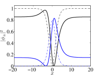
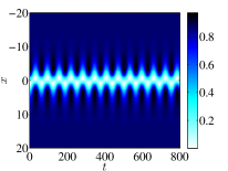
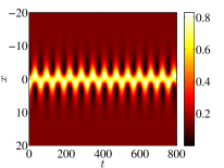
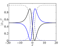
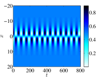
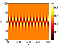
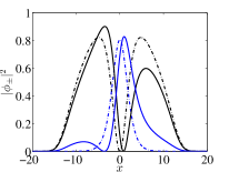
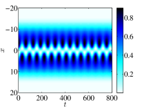
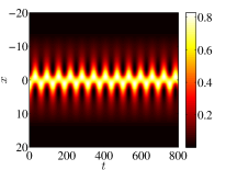
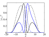
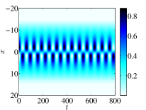
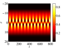
Figure 1: (Color online) Summary of results corresponding to the case with equal interaction coefficients and values of the chemical potentials of $\mu_{-}=1$ and $\mu_{+}=0.9$. Panels (a)-(c), (g)-(i), and (d)-(f), (j)-(l) correspond to a rotation of the original steady state by $\delta=\pi/8$ and $\delta=\pi/4$, respectively. In addition, the first two rows correspond to the homogeneous case whereas the last two are shown in the presence of an external potential with trap strength of $\Omega=0.1$. The left column presents the corresponding $SO(2)$-rotated waveforms at $t=0$ for each case depicted by solid blue (for the bright component) and black (for the dark one) lines. Also, the original unrotated dark (dash-dotted black line) and bright (dash-dotted blue line) solitary waveforms are depicted as well for comparison. The spatio-temporal evolution of the densities $|\Phi_{-}(x,t)|^{2}$ and $|\Phi_{+}(x,t)|^{2}$ is presented in the middle and right columns, respectively, with different colormaps in order to differentiate between the two.

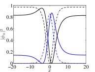
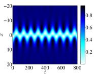
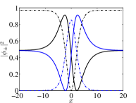
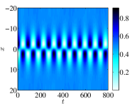
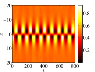
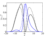
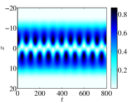
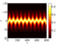
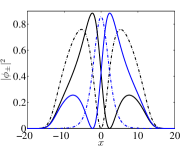
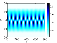
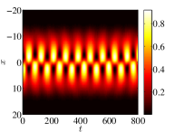
Figure 2: (Color online) Same as Fig. 1 but for unequal interaction coefficients, with $g_{11}=1.03$, $g_{12}=1$ and $g_{22}=0.97$.

III.2 Vortex–Vortex structures in 2D

In this section, we take a step further and discuss rotated vortex-bright soliton complexes in 2D, by considering specific cases spanning various possibilities. Figures 3, 4 and 5 depict examples of initially rotated – so as to produce the vortex–vortex (VV) state – and dynamically evolved vortex-bright solitons with equal interaction coefficients and values of the chemical potentials of $\mu_{-}=1$ and $\mu_{+}=0.85$. Figure 6, corresponding to $\mu_{-}=5.2$ and $\mu_{+}=4.2$, highlights the effect of unequal interaction coefficients. Furthermore, Figs. 3 and 4 correspond to a rotation by $\pi/4$ of the original vortex-bright soliton complex, in the absence and presence of a trap (with $\Omega=0.2$), respectively. On the same footing, Fig. 5 corresponds to a rotation by $\pi/8$ of the original state whereas Fig. 6 for $\mu_{-}=5.2$ and $\mu_{+}=4.2$ involves rotation by $\pi/4$. Both of the latter examples are in the presence of a trap. Snapshots of the densities $|\Phi_{-}(x,y,t)|^{2}$ and $|\Phi_{+}(x,y,t)|^{2}$ at different instants of time $t$ are depicted in the top and bottom rows, respectively, of Figs. 3, 4, and 5, as well as in Fig. 6. Our study is complemented by demonstrating isocontours of the individual densities of the vortex and bright soliton of each component in panels (b) and (c) of Figs. 3, 4 and 5 with gray and blue colors, respectively.

As has been illustrated in the recent study of vbs_coupled (even in the absence of a trap), but also in earlier works in the presence of a trap kodyprl , the vortex-bright state is generally stable. As mentioned in Section II, its rotated VV counterpart inherits these traits. Furthermore, the internal period $T$ of vibration of the VV state in the equal interactions coefficients case is given by Eq. (8), as shown in the previous section. In our numerical results the period calculated numerically follows this analytical prediction, a feature that we have used as a benchmark of our numerical method footnote . Once again, the presence of the trap does not appear to significantly affect the motion of the vortices in the case of equal interaction coefficients: the vortex constituents of the VV state in each component continue to blithely orbit around each other both in the presence and in the absence of the trap.

Specifically, snapshots of the densities are presented in panels (a) of Figs. 3, 4 and 5 at each $t$ which is equal to one quarter of the period, i.e., $t=0$, $t=T/4$, $t=T/2$, $t=3T/4$ and $t=T$ (with $T\approx 41.88$ in these examples). This way, the vortex–vortex complex performs a circular motion as time evolves (see, the insets therein) and returns to its original position at $t=T$ (see, the last column of panels (a)). Furthermore, the oscillations of the vortex-vortex complexes are persistent as our long-time dynamics reveal in panels (b) and (c) of Figs. 3, 4 and 5 (see, the range of $t$ axes therein) suggesting that the underlying states are indeed robust.

Arguably more intriguing, however, appears to be the case of unequal interaction coefficients. In this case, and in the presence of the trap, the results are illustrated in Fig. 6; see, also, vv_movie for a complete movie of the dynamics in this case. Although the initial vortex–bright soliton is stable (in the realm of linear stability analysis), its vortex–vortex sibling appears to undergo modifications of its density profile. At first, the vortex–vortex complex follows a circular motion, where the period increases compared to the analytical prediction of Eq. (8), due to the unequal interaction coefficients. In analogy to the 1D setting, this is expected based on the fact that the $SU(2)$-invariance is broken. Then, the configuration starts changing in shape (see the panels in the second column of the Figure) leading at $t=50$ the bright soliton in the second component to disappear, while in the first component the vortex structure cannot be straightforwardly discerned in the density. However, the complex in the second component regains (qualitatively) its structural form back around $t=80$, leading to the recurrence of the VV state (in a rotated form). It is evident in the snapshots (especially of the second and third column of Fig. 6) that the dynamics features phase separation phenomena analyzed in detail, e.g., in the experimental (and computational) analysis of Ref. originalhall ; see also refhall . Indeed, while the rotation of the VV pattern persists (or, at least, recurs), the overall density pattern develops the target patterns analyzed in (the planar projections associated with) Ref. originalhall ; see also siambook and references therein. Our conclusion in that connection is that the robustness of the rotational state is, at least in part, affected by the location of the relevant interaction coefficients with respect to the miscibility/immiscibility transition – associated with crossing the critical point $D=0$ of the immiscibility parameter $D\equiv g_{11}g_{22}-g_{12}^{2}$ siambook .

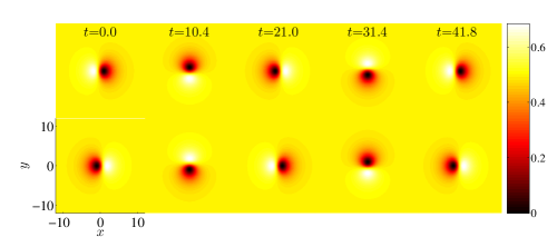
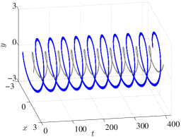
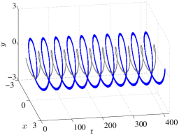
Figure 3: (Color online) Summary of results under the action of the $SO(2)$ rotation by $\pi/4$ corresponding to the homogeneous case with equal interaction coefficients and values of the chemical potentials of $\mu_{-}=1$ and $\mu_{+}=0.85$. Top row: Snapshots of densities $|\Phi_{-}(x,y,t)|^{2}$ (top panels) and $|\Phi_{+}(x,y,t)|^{2}$ (bottom panels) at different instants of time. Bottom row: Isosurfaces of the spatiotemporal evolution of the densities $|\Phi_{-}(x,y,t)|^{2}$ and $|\Phi_{+}(x,y,t)|^{2}$ presented in panels (b) and (c), respectively. Each isosurface depicted by blue and gray color corresponds to a value of $0.001\times\max(|\Phi_{-}(x,y,t)|^{2})$ and $0.999\times\max(|\Phi_{+}(x,y,t)|^{2})$, respectively.

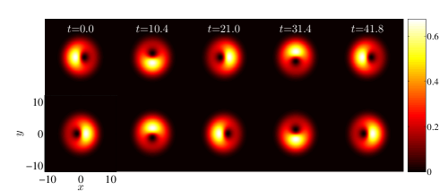
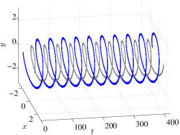
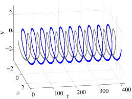
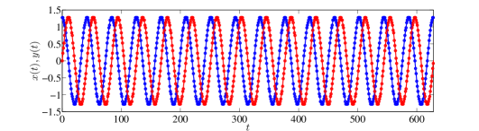
Figure 4: (Color online) Same as Fig. 3 but under the presence of harmonic confinement with $\Omega=0.2$. Top row: Snapshots of densities $|\Phi_{-}(x,y,t)|^{2}$ (top panels) and $|\Phi_{+}(x,y,t)|^{2}$ (bottom panels) at different instants of time. Middle row: Isosurfaces of the spatiotemporal evolution of the densities $|\Phi_{-}(x,y,t)|^{2}$ and $|\Phi_{+}(x,y,t)|^{2}$ presented in panels (b) and (c), respectively. Each isosurface depicted by blue and gray color corresponds to a value of $0.001\times\max(|\Phi_{-}(x,y,t)|^{2})$ and $0.999\times\max(|\Phi_{+}(x,y,t)|^{2})$, respectively. Bottom row: The location of the vortex $(x,y)$ in the first component as a function of time where its abscissa and ordinate are depicted with blue and red circles, respectively. The solid blue and red lines correspond to the theoretical prediction.

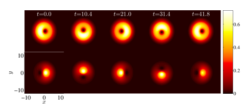
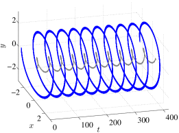
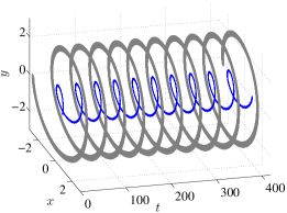
Figure 5: (Color online) Same as Fig. 4 but for $\delta=\pi/8$. Top row: Snapshots of densities $|\Phi_{-}(x,y,t)|^{2}$ (top panels) and $|\Phi_{+}(x,y,t)|^{2}$ (bottom panels) at different instants of time. Bottom row: Isosurfaces of the spatiotemporal evolution of the densities $|\Phi_{-}(x,y,t)|^{2}$ and $|\Phi_{+}(x,y,t)|^{2}$ presented in panels (b) and (c), respectively. Similarly, each isosurface depicted by blue and gray color corresponds to a value of $0.001\times\max(|\Phi_{-}(x,y,t)|^{2})$ and $0.999\times\max(|\Phi_{+}(x,y,t)|^{2})$, respectively.

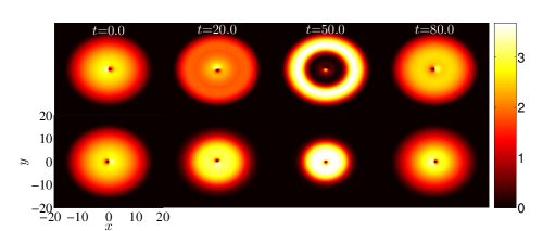
Figure 6: (Color online) Same as Fig. 4 but for unequal interaction coefficients. Snapshots of densities $|\Phi_{-}(x,y,t)|^{2}$ (top panels) and $|\Phi_{+}(x,y,t)|^{2}$ (bottom panels) at different instants of time. Here, the phase separation in this immiscible regime affects the density by resulting in target patterns (previously observed also in experiments; see the text) in the dynamics. See Ref. vv_movie for a more complete movie of the dynamics.

III.3 VL–VL and VR–VR solitons in 3D

Finally, we study the effect of $SO(2)$ rotations to construct vorticity-bearing vector structures in 3D. In particular, we focus on the cases of the VL-bright soliton and the VR-bright soliton. As in 1D and 2D, we first identify the stationary states, study their stability traits and subsequently rotate the corresponding states. Then, we monitor the dynamics of these states by advancing the NLS system forward in time. A stationary VL–bright soliton state is shown is Fig. 7. We have checked that the state at the studied parameters is stable using spectral stability analysis methods analogous to those utilized in Ref. dsss_ww , as well as direct dynamical integration up to $t=100$.

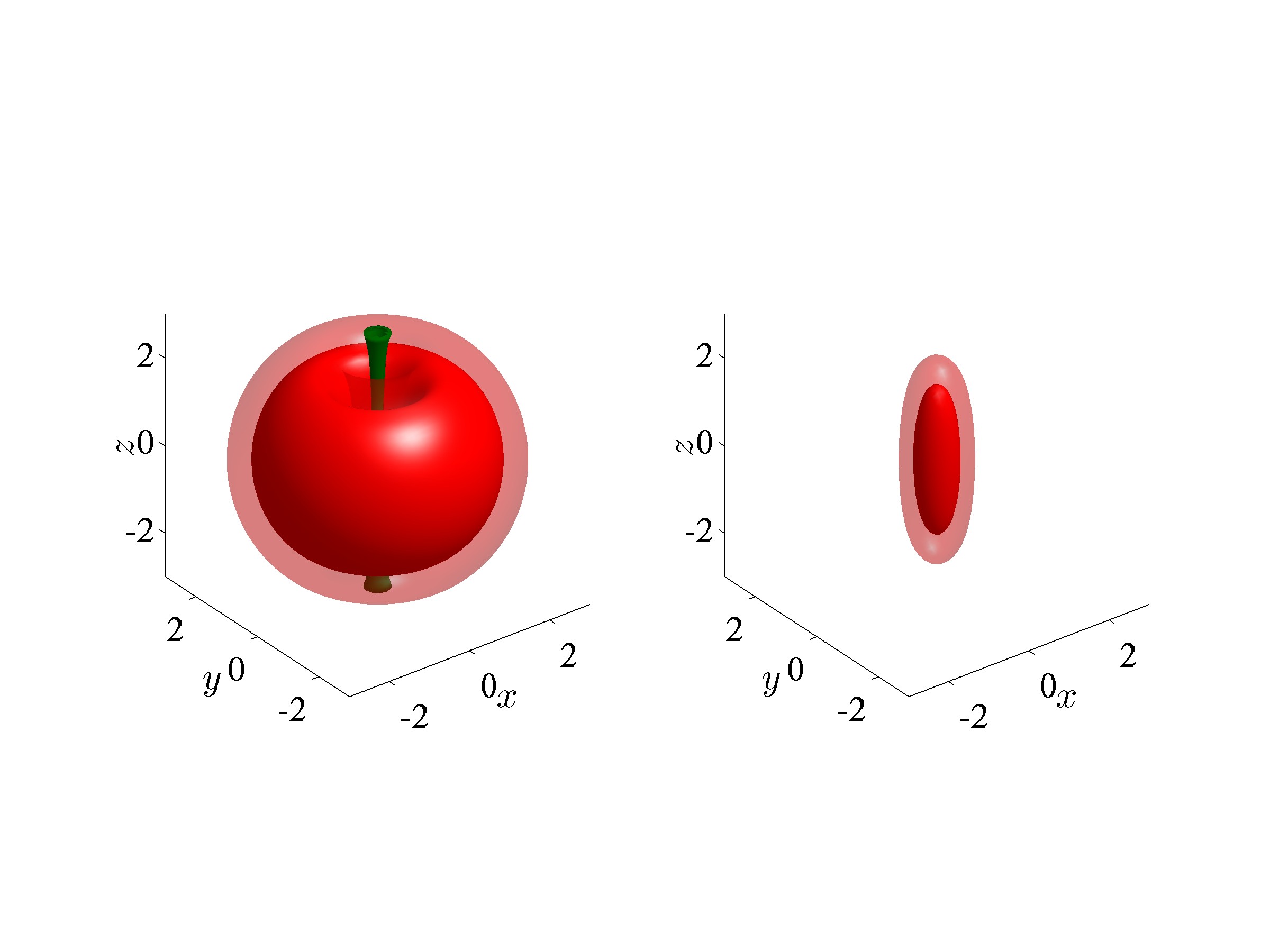
Figure 7: (Color online) The density isocontour plots of a stable stationary vortex-line-bright soliton at $\mu_{1}=7$ and $\mu_{2}=6.2$ in an isotropic trap with $\Omega=1$. The core of the line is highlighted in green (dark) contours.

Subsequently, we perform the $SO(2)$ rotation with $\delta=\pi/4$, and the VL–bright soliton state morphs into a VL-VL solitary wave. Dynamical evolution shows that the two vortex lines perform a rotational motion around each other in the trap. Some typical intermediate stages within a period are shown in Fig. 8. See Ref. VLVL1_movie for a more complete movie of the dynamics. We have also verified that similar robust dynamics also hold for $\delta=\pi/8$. Hence, such VL–VL states are natural candidates for observation in the dynamics of the system – although, of course, it does not escape us that unequal interaction coefficients may again impose density modulations via phase-separation phenomena; we comment on this further below.

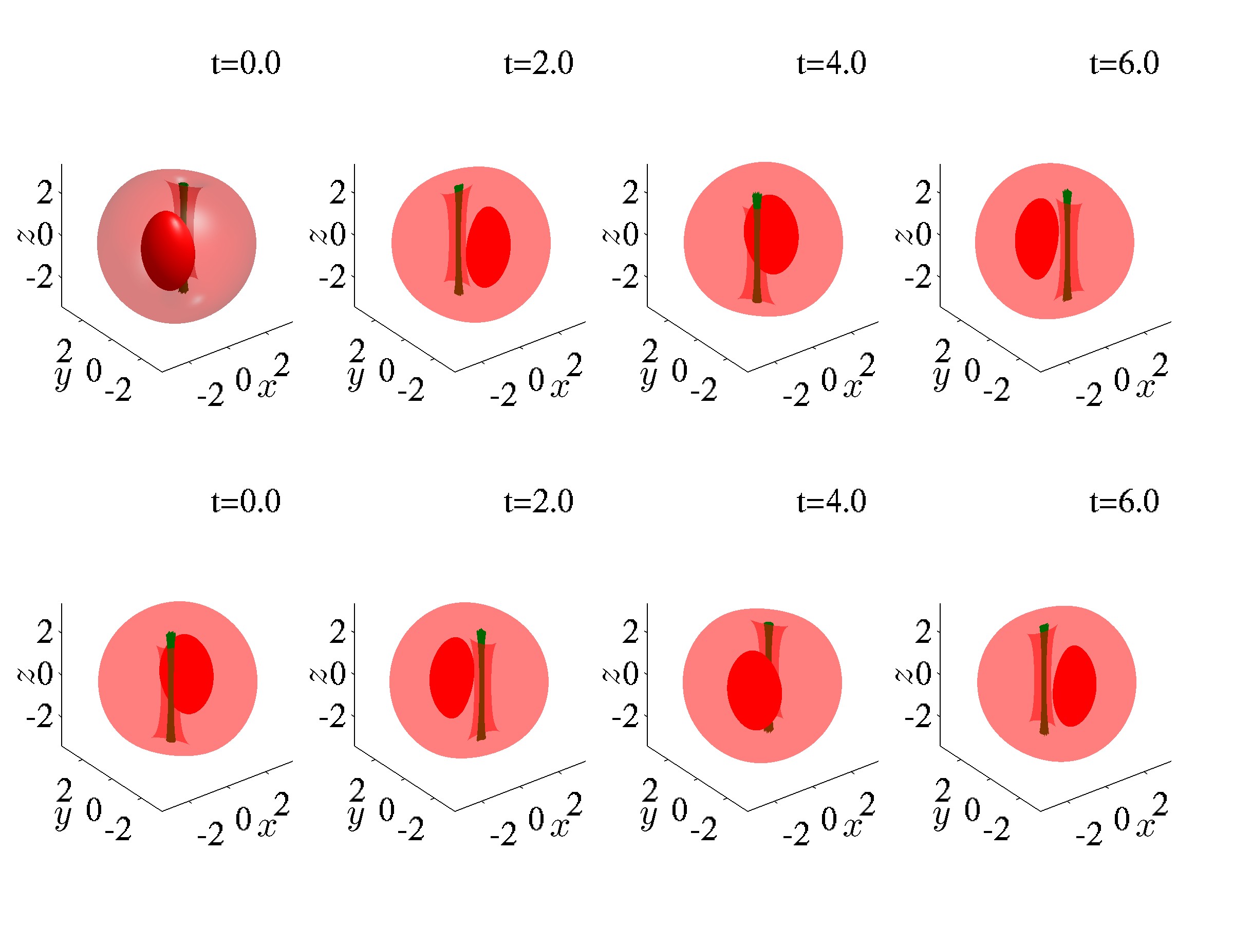
Figure 8: (Color online) Robust VL–VL oscillations transformed from the VL-bright soliton state shown in Fig. 7. Typical states are shown for one period, with the top panel for one component and the bottom panel for the other component. See Ref. VLVL1_movie for a more complete movie of the dynamics.

Now we discuss the VR–bright soliton. Similarly, a stable stationary state of the VL–bright soliton is shown in Fig. 9, and is converged upon fixed point iteration. Dynamics in the case of $\delta=\pi/4$ are shown in Fig. 10, and robust oscillations also hold for the case $\delta=\pi/8$. Here, the vortex rings are involved in an intriguing “dance” routine, where they vibrate between pairs of inner-outer, then top-bottom, then outer-inner, and finally bottom-top (for the two species), before the cycle restarts, as is illustrated in the figure. A more detailed perspective of the relevant choreography is given in the movie of Ref. VRVR1_movie .

It is important to remind the reader here that these results were obtained with a fairly confining isotropic trap of strength $\Omega=1$. We have explored the dynamics observed in the case of $g_{ij}\neq 1$ for phase separation and while we did see signatures of the latter, these were found to be quite weak in this setting (relatively to the 2D case discussion presented above). This is in line with earlier observations, see e.g., rafael , indicating theoretically and computationally that the phase separation transition threshold is shifted (and phase separation is generally progressively more suppressed) the stronger the confinement of the atomic species.

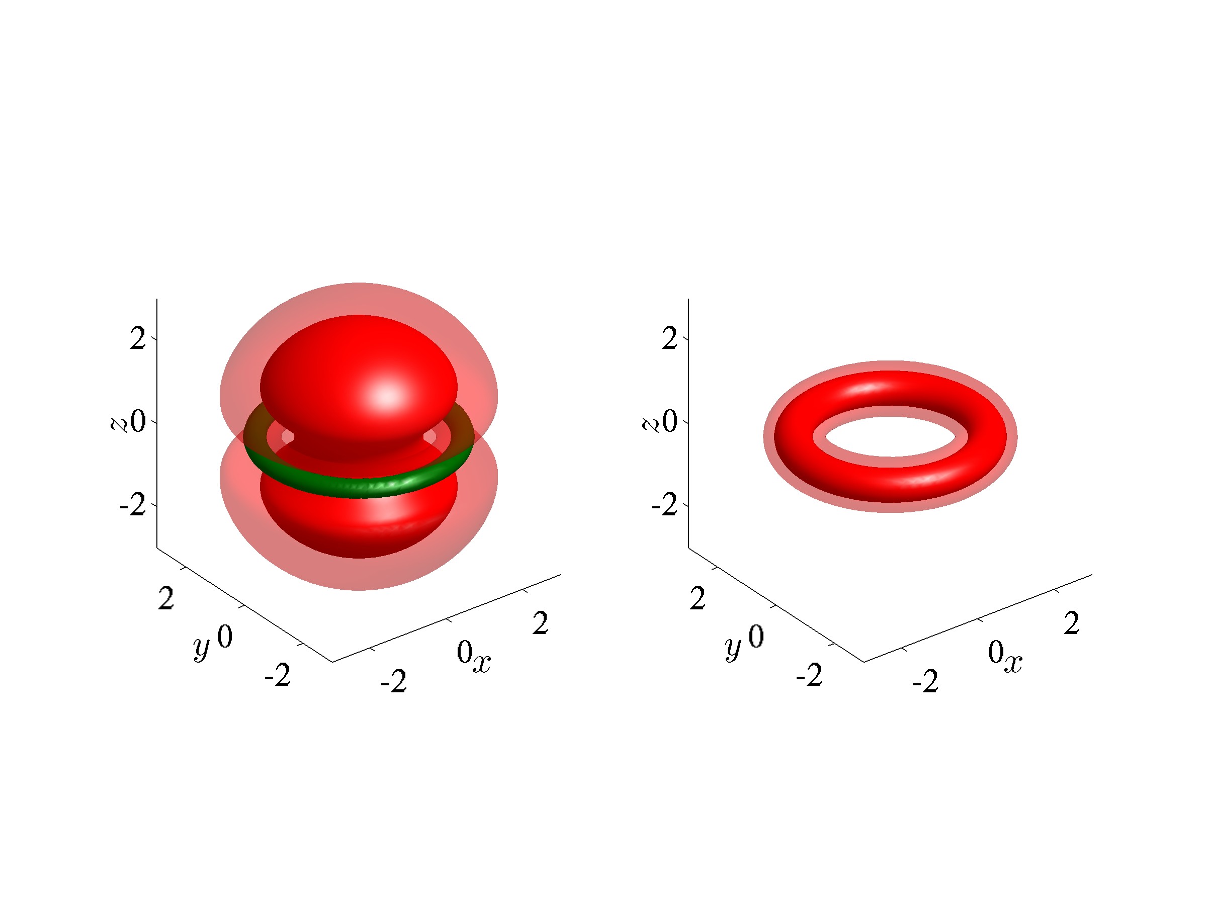
Figure 9: (Color online) The density isocontour plots of a stable stationary vortex-ring-bright soliton at $\mu_{1}=9$ and $\mu_{2}=7.6$ in an isotropic trap with $\Omega=1$. The core of the ring is highlighted in green (dark) contours.

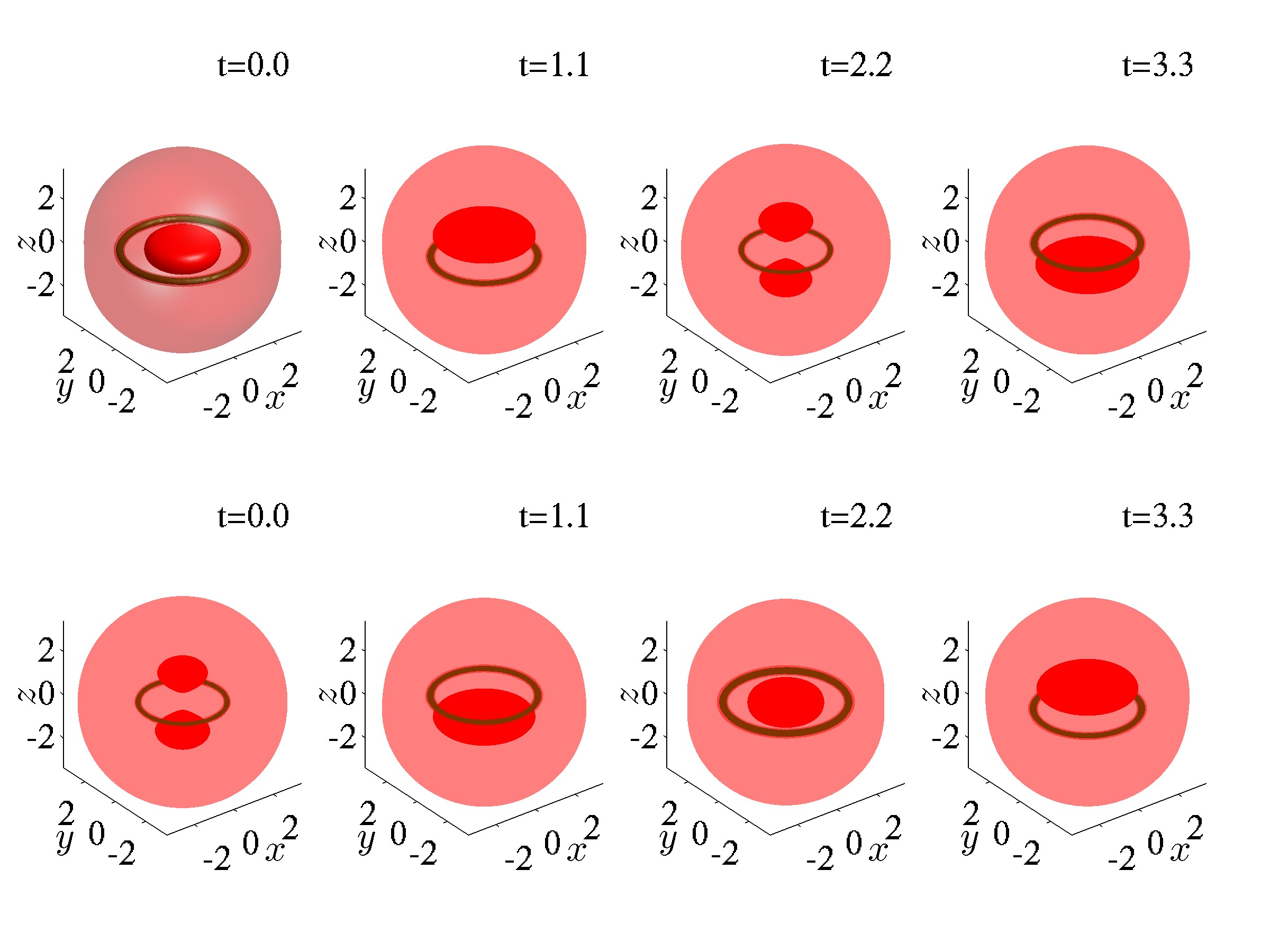
Figure 10: (Color online) Robust VR–VR oscillations transformed from the VR-bright soliton state shown in Fig. 9. Typical states are shown for one period, with the top panel for one component and the bottom panel for the other component. See Ref. VRVR1_movie for a more complete movie of the dynamics.

IV Concluding remarks and future challenges

In the present work, we have considered the two-component, one-, two- and three-dimensional nonlinear Schrödinger system with the self-defocusing nonlinearity, and studied the effect of $SO(2)$ rotations on stable stationary dark-bright solitons and higher-dimensional vortex complexes. Our numerical findings revealed that the complexes considered in this work are robust (over a wide time interval), suggesting possibilities of observing the underlying states experimentally in Bose-Einstein condensates. While our starting point was the revisiting of the simpler (and experimentally observed) dark-dark solitons, we illustrated that the transformation and its feature of potentially producing breathing states from stationary ones are independent of dimension. While analytical solutions are not available in higher dimensions in order to subject them to the transformation, it is straightforward to obtain numerical ones and not only evolve them dynamically, but also predict on the basis of the difference of their chemical potentials, the period of the resulting periodic pattern. We performed this step for a vortex–bright soliton in 2D, obtaining a vortex–vortex state in that system, while in 3D, the robustness of both vortex-line–soliton and of vortex-ring–soliton allowed us to form structures with vortex lines and vortex rings precessing around each other in the two components.

Our observations, while exact in the context of the Manakov model, as we showcased via select dynamical examples, are no longer so in the case of unequal interaction coefficients. In fact, it is evident that in such cases, even weak deviations from the miscibility-immiscibility threshold that the Manakov system represents (as is relevant for atomic BECs) may give rise to spontaneously phase-separating patterns for homogeneous or sufficiently weakly trapped systems, on top of which the vibration of the coherent structures of interest may take place. This is a natural direction for further quantitative exploration, i.e., a more quantitative identification of the boundaries of robustness of the states developed herein. Such variation is quite accessible presently, e.g., via Feshbach resonance techniques frm . Additionally, the realization that the methodology is independent of dimension and structure also creates the potential of applying features of this type to other states (including in the focusing case) in order to obtain other such exotic, time vibrating states. Such studies are currently in progress and will be reported in the future.

- (1) S. V. Manakov, Sov. Phys. JETP, 38, 248–253 (1973).
- (2) V. E. Zakharov and S. V. Manakov, Sov. Phys. JETP, 42, 842–850 (1976).
- (3) C. Sulem and P. L. Sulem, The Nonlinear Schrödinger Equation, Springer-Verlag (New York, 1999).
- (4) M. J. Ablowitz, B. Prinari, and A. D. Trubatch, Discrete and Continuous Nonlinear Schrödinger Systems, Cambridge University Press (Cambridge, 2004).
- (5) P. G. Kevrekidis, D. J. Frantzeskakis, and R. Carretero-González, The Defocusing Nonlinear Schrödinger Equation, SIAM (Philadelphia, 2015).
- (6) P. G. Kevrekidis and D. J. Frantzeskakis, arXiv:1512.06754.
- (7) L. P. Pitaevskii and S. Stringari, Bose-Einstein Condensation. Oxford University Press (Oxford, 2003).
- (8) D. N. Christodoulides, Phys. Lett. A, 132, 451–452 (1988).
- (9) V. V. Afanasyev, Yu. S. Kivshar, V. V. Konotop, and V. N. Serkin, Opt. Lett., 14, 805–807 (1989).
- (10) Yu. S. Kivshar and S. K. Turitsyn, Opt. Lett., 18, 337–339 (1993).
- (11) R. Radhakrishnan and M. Lakshmanan, J. Phys. A: Math. Gen., 28, 2683–2692 (1995).
- (12) A. V. Buryak, Yu. S. Kivshar, and D. F. Parker, Phys. Lett. A, 215, 57–62 (1996).
- (13) A. P. Sheppard and Yu. S. Kivshar, Phys. Rev. E, 55, 4773–4782 (1997).
- (14) Q. Han Park and H. J. Shin, Phys. Rev. E, 61, 3093–3106 (2000).
- (15) Yu. S. Kivshar and G. P. Agrawal, Optical Solitons: from fibers to photonic crystals, Academic Press (San Diego, 2003).
- (16) Z. Chen, M. Segev, T. H. Coskun, D. N. Christodoulides, and Yu. S. Kivshar, J. Opt. Soc. Am. B, 14, 3066–3077 (1997).
- (17) E. A. Ostrovskaya, Yu. S. Kivshar, Z. Chen, and M. Segev, Opt. Lett., 24, 327–329 (1999).
- (18) Th. Busch and J. R. Anglin, Phys. Rev. Lett., 87, 010401 (2001).
- (19) C. Becker, S. Stellmer, P. Soltan-Panahi, S. Dörscher, M. Baumert, E.-M. Richter, J. Kronjäger, K. Bongs, and K. Sengstock, Nature Phys., 4, 496–501 (2008).
- (20) C. Hamner, J. J. Chang, P. Engels, and M. A. Hoefer, Phys. Rev. Lett., 106, 065302 (2011).
- (21) S. Middelkamp, J. J. Chang, C. Hamner, R. Carretero-González, P. G. Kevrekidis, V. Achilleos, D. J. Frantzeskakis, P. Schmelcher,and P. Engels, Phys. Lett. A, 375, 642–646 (2011).
- (22) D. Yan, J. J. Chang, C. Hamner, P. G. Kevrekidis, P. Engels, V. Achilleos, D. J. Frantzeskakis, R. Carretero-González, and P. Schmelcher, Phys. Rev. A, 84, 053630 (2011).
- (23) M. A. Hoefer, J. J. Chang, C. Hamner, and P. Engels, Phys. Rev. A, 84, 041605(R) (2011).
- (24) D. Yan, J. J. Chang, C. Hamner, M. Hoefer, P. G. Kevrekidis, P. Engels, V. Achilleos, D. J. Frantzeskakis, and J. Cuevas, J. Phys. B: At. Mol. Opt. Phys., 45, 115301 (2012).
- (25) A. Álvarez, J. Cuevas, F. R. Romero, C. Hamner, J. J. Chang, P. Engels, P. G. Kevrekidis, and D. J. Frantzeskakis, J. Phys. B, 46, 065302 (2013).
- (26) P. G. Kevrekidis, D. J. Frantzeskakis, and R. Carretero-González (Eds.), Emergent Nonlinear Phenomena in Bose-Einstein Condensates: Theory and Experiment Springer-Verlag (Heidelberg, 2008).
- (27) K. J. H. Law, P. G. Kevrekidis, and L. S. Tuckerman, Phys. Rev. Lett., 105, 160405 (2010).
- (28) M. Pola, J. Stockhofe, P. Schmelcher, and P. G. Kevrekidis, Phys. Rev. A, 86, 053601 (2012).
- (29) B. P. Anderson, P. C. Haljan, C. E. Wieman, and E. A. Cornell Phys. Rev. Lett. 85, 2857 (2000).
- (30) M. Eto, K. Kasamatsu, M. Nitta, H. Takeuchi, and M. Tsubota, Phys. Rev. A, 83, 063603 (2011).
- (31) S. K. Adhikari, Phys. Rev. E 92, 042926 (2015); see also: Sandeep Gautam, S. K. Adhikari, Phys. Rev. A 93, 013630 (2016).
- (32) R. A. Battye, N. R. Cooper, and P. M. Sutcliffe, Phys. Rev. Lett., 88, 080401 (2002).
- (33) D. V. Skryabin, Phys. Rev. A, 63, 013602 (2000).
- (34) S. Komineas, Eur. Phys. J. Spec. Top. 147, 133 (2007).
- (35) K. M. Mertes, J. W. Merrill, R. Carretero-González, D. J. Frantzeskakis, P. G. Kevrekidis, and D. S. Hall, Phys. Rev. Lett. 99, 190402 (2007).
- (36) M. Egorov, B. Opanchuk, P. Drummond, B. V. Hall, P. Hannaford, and A. I. Sidorov, Phys. Rev. A 87, 053614 (2013).
- (37) E. G. Charalampidis, P. G. Kevrekidis, D. J. Frantzeskakis, and B. A. Malomed, Phys. Rev. E 91, 012924 (2015).
- (38) E. G. Charalampidis, P. G. Kevrekidis, D. J. Frantzeskakis, and B. A. Malomed, arXiv:1512.07693.
- (39) For instance, Fig. 4 presents the location of the vortex in the first component as a function of time where the abscissa and ordinate are denoted by blue and red circles. We compare the numerical results by using the analytical formulae and , with and standing for the initial location of the complex, while , as shown in section II. It can be discerned from Fig. 4 that not only the complex performs a circular motion, suggesting its periodic nature, but it is clearly robust.
- (40) W. Wang, P. G. Kevrekidis, R. Carretero-González, and D. J. Frantzeskakis, Phys. Rev. A 93, 023630 (2016).
- (41) G. Thalhammer, G. Barontini, L. De Sarlo, J. Catani, F. Minardi, and M. Inguscio, Phys. Rev. Lett. 100, 210402 (2008); S. B. Papp, J. M. Pino, and C. E. Wieman, Phys. Rev. Lett. 101, 040402 (2008).
- (42) https://www.youtube.com/watch?v=ePzPFi3H5VY
- (43) https://www.youtube.com/watch?v=WOp8TlsDsSs
- (44) https://www.youtube.com/watch?v=4BILu5mvxGk
- (45) See, e.g., R. Navarro, R. Carretero-González and P.G. Kevrekidis, Phys. Rev. A. 80, 023613 (2009) around Eq. (20) and associated discussion on the dependence of the phase separation threshold.