A broadband Ferromagnetic Resonance dipper probe for magnetic damping measurements from 4.2 K to 300 K

Abstract

A dipper probe for broadband Ferromagnetic Resonance (FMR) operating from 4.2 K to room temperature is described. The apparatus is based on a 2-port transmitted microwave signal measurement with a grounded coplanar waveguide. The waveguide generates a microwave field and records the sample response. A 3-stage dipper design is adopted for fast and stable temperature control. The temperature variation due to FMR is in the milli-Kelvin range at liquid helium temperature. We also designed a novel FMR probe head with a spring-loaded sample holder. Improved signal-to-noise ratio and stability compared to a common FMR head are achieved. Using a superconducting vector magnet we demonstrate Gilbert damping measurements on two thin film samples using a vector network analyzer with frequency up to 26 GHz: 1) A Permalloy film of 5 nm thickness and 2) a CoFeB film of 1.5 nm thickness. Experiments were performed with the applied magnetic field parallel and perpendicular to the film plane.

I introduction

In recent years, the switching of a nanomagnet by spin transfer torque (STT) using a spin polarized current has been realized and intensively studied.(Slonczewski, 1996; Katine et al., 2000; Mangin et al., 2006) This provides avenues to new types of magnetic memory and devices, reviving the interest on magnetization dynamics in ultrathin films.(Locatelli, Cros, and Grollier, 2014; Brataas, Kent, and Ohno, 2012) High frequency techniques play an important role in this research direction. Among them, Ferromagnetic Resonance (FMR) is a powerful tool. Most FMR measurements have been performed using commercially available systems, such as electron paramagnetic resonance (EPR) or electron spin resonance (ESR).(Farle, 1998) These techniques take advantage of the high Q-factor of a microwave cavity, where the field modulation approach allows for the utilization of a lock-in amplifier.(Heinrich, 2006) The high signal-to-noise ratio enables the measurement of even sub-nanometer thick magnetic films. However, the operating frequency of a metal cavity is defined by its geometry and thus is fixed. To determine the damping of magnetization precession, which is in principle anisotropic, several cavities are required to study the relation between the linewidth and microwave frequency at a given magnetization direction.(Heinrich et al., 2003; Lenz et al., 2006; Heinrich et al., 2011)The apparent disadvantage is that changing cavities can be tedious and prolong the measurement time.

Recently, an alternative FMR spectrometer has attracted considerable attention.(Kalarickal et al., 2006; Harward et al., 2011; Wei et al., 2014; Montoya et al., 2014; Głowiński et al., 2014; Bailleul, 2013; Bilzer et al., 2007) The technique is based on a state of the art vector network analyzer (VNA) and a coplanar waveguide (CPW). Both VNA and CPW can operate in a wide frequency range hence this technique is also referred to as broadband FMR or VNA-FMR. The broadband FMR technique offers several advantages. First, it is rather straightforward to measure FMR over a wide frequency range. Second, one may fix the applied magnetic field and acquire spectra with sweeping frequency in a matter of minutes.(Bilzer et al., 2007) Furthermore, a CPW fabricated on a chip using standard photolithography enables FMR measurements on patterned films as well as on a single device.(Neudecker et al., 2006) In brief, it is a versatile tool suitable for the characterization of magnetic anisotropy, investigation of magnetization dynamics and the study of high frequency response of materials requiring a fixed field essential to avoid any phase changes caused by sweeping the applied field.

Although homebuilt VNA-FMRs are designed mainly for room temperature measurements, a setup with variable temperature capability is of great interest both for fundamental studies and applications. Denysenkov et al. designed a probe with variable sample temperature, namely, 4-420 K, (Denysenkov and Grishin, 2003) however, the spectrometer only operates in reflection mode. In a more recent effort, Harward et al. developed a system operating at frequencies up to 70 GHz.(Harward et al., 2011) However the lower bound temperature of the apparatus is limited to 27 K. Here we present a 2-port broadband FMR apparatus based on a superconducting magnet. A 3-stage dipper probe has been developed which allows us to work in the temperature range 4.2 - 300 K. Taking advantage of a superconducting vector magnet, measurements can be performed with the magnetic moment saturated either parallel or perpendicular to the film plane. We also designed a spring-loaded sample holder for fast and reliable sample mounting, quick temperature response and improved stability. This setup allows for swift changes of the FMR probe heads and requires little effort for the measurement of devices. To demonstrate the capability of this FMR apparatus we measured the temperature dependence of magnetization dynamics of thin film samples of Permalloy (Py) and CoFeB in different applied magnetic field configurations.

II apparatus

II.1 Cryostat and superconducting magnet system

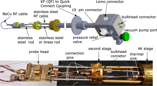
Figure 1: View of the FMR dipper probe. Top panel: The schematic of the entire design with a straight type FMR head. All RF connectors are 2.4 mm. The vacuum cap mounted on the 4 K stage, using In seal, and the radiation shield mounted on the second stage are not shown for clarity. Bottom panel: photograph of the components inside the vacuum cap.

Our customized cryogenic system was developed by Janis Research Company Inc. and includes a superconducting vector magnet manufactured by Cryomagnetics Inc. A vertical field up to 9 T is generated by a superconducting solenoid. The field homogeneity is $\pm$0.1% over a 10 mm region. A horizontal split pair superconducting magnet provides a field up to 4 T with uniformity $\pm$0.5% over a 10 mm region. The vector magnet is controlled by a Model 4G-Dual power supply. Although the power supply gives field readings according to the initial calibration, to avoid the influence of remnant field we employ an additional Hall sensor. The cryostat has a 50 mm vertical bore to accommodate variable temperature inserts and dipper probes. Our dipper probe described below is configured for this cryostat, however, the principle can be applied also to other commercially available superconducting magnets and cryostats.

II.2 Dipper probe

Fig. 1 shows a schematic of our dipper probe assembly and a photograph of the components inside the vacuum cap. The dipper probe is 1.2 m long and is mounted to the cryogenic system via a KF50 flange. The sliding seal allows a slow insertion of the dipper probe directly into the liquid helium space. Supporting arms (not shown) lock the probe and minimize vibration, with the sample aligned to the field center. The connector box on top has vacuum tight Lemo and Amphenol connectors for 18 DC signal feedthrough. Two 2.4 mm RF connection ports allow for frequencies up to 50 GHz . A vacuum pump port can be shut by a Swagelok valve. We adopted a three stage design as shown in the photograph of Fig. 1. The 4 K stage and the vacuum cap immersed in the He bath provide cooling power for the probe. The intermediate second stage acts as an isolator of heat flow and as thermal sink for the RF cables, providing improved temperature control. Furthermore, it allows one to change probe heads conveniently as we discuss later. A separate temperature sensor on the second stage is used for monitoring purpose. The third stage, namely, the FMR probe head with the spring loaded sample holder, is attached to the lower end of the intermediate stage using stainless steel rods.

A pair of 0.086” stainless steel Semi-Rigid RF cables run from the top of the connector box to the non-magnetic bulkhead connector (KEYCOM Corp.) mounted on the second stage. BeCu non-magnetic Semi-Rigid cables (GGB Industries, Inc.) are used for the connection between the second stage and the probe head. The cables are carefully bent to minimize losses. The rods connecting the stages are locked by set screws. Loosening the set screw allows the rod length to be adjusted to match the length of the RF cables. Reflection coefficient (S₁₁) and transmission coefficient (S₂₁) can be recorded simultaneously with this 2-port design. The leads for the temperature sensors, heater, Hall sensor and for optional transport measurements are wrapped around Cu heat-sinks at the 4 K stage before being soldered to the connection pins.

II.3 Probe head with spring-loaded sample holder

The key part of the dipper probe, namely, the FMR probe head is schematically shown in Fig. 2. The assembly is placed in a radiation shield tube with an inner diameter of 32 mm. To maximize thermal conduction between parts, homebuilt components are machined from Au plated Cu. The 1” long customized grounded coplanar waveguide (GCPW) has a nominal impedance of 50 Ohm. The straight-line shape GCPW was made on duroid^® R6010 (Rogers) board, with a thickness of 254$\,\mu\text{m}$ and dielectric constant 10.2. The width of the center conductor is 117 $\mu\text{m}$ and the gap between the latter and the ground planes is 76 $\mu\text{m}$. For the connection, first the GCPW is soldered to the probe head, and subsequently the center pin of the flange connector (Southwest Microwave) is soldered to the center conductor of the GCPW. The response of the dipper with the straight-line shape GCPW installed is shown in Fig. 3. The relatively large insertion loss (-16.9 dB at 26 GHZ) is due to a total cable length of more than 3 m and multiple connectors. The high frequency current flowing in the CPW generates a magnetic field of the same frequency. This RF field drives the precession of the magnetic material placed on top of the signal line, and gives rise to a change in the system’s impedance, which in turn alters the transmitted and reflected signals.

Figure 2: Schematic of the spring-loaded FMR probe head with straight shape grounded coplanar waveguide (GCPW). 1 Au plated Cu housing; 2 straight shape GCPW; 3 flange connector; 4 strain gauge thin film heater; 5 Cernox^TM temperature sensor; 6 Hall-sensor housing; 7 housing for 4-pin Dip socket or pingo pin; 8 sample; 9 sample holder; 10 Cu spring; 11 spring housing; 12 sample holder handle nut.

A spring-loaded sample holder depicted in Fig. 2 by items 9 to 12 is designed to mount the sample. The procedure for loading a sample is as follows: 1) Pull up the handle nut and apply a thin layer of grease (Apiezon N type) to the sample holder; 2) Place the sample at the center of the sample holder; 3) Mount the spring-loaded sample holder to the FMR head; 4) Release the handle nut gradually so that the spring pushes the sample towards the waveguide. The mounting-hole of the spring-housing is slightly larger than the outer diameter of the spring. This allows the sample holder to match the surface of the GCPW self-adaptively. With the spring-loaded FMR head design, the sample mounting is simple and leaves no residue from the commonly used tapes. It maximizes the signal by minimizing the gap between waveguide and sample, and enhances the stability. Furthermore, it is suitable for variable temperature measurements due to the enhanced thermal coupling between the sample, cold head and sensors ( items 9 to 12 in Fig. 2.).

The temperature sensor is mounted at the backside of the probe head. Due to limited space, the heater consists of three parallel connected strain gauges with a resistance of 120 Ohm. The Hall sensor can be mounted according to the required measurement configuration. The position of the Hall sensor shown in Fig. 2 is an example for measurements in the presence of a magnetic field applied parallel to the sample surface.

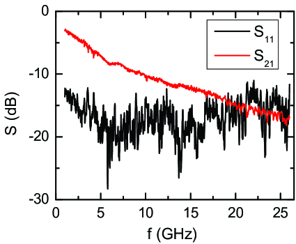
Figure 3: The reflection (S₁₁) and transmission (S₂₁) coefficients of the dipper probe with the straight-line shape GCPW mounted. The measurement was performed at room temperature.

II.4 Probe-head using end-launch connector

Although the probe head with straight-line CPW works well in our experiment, the necessary replacement of CPW due to unavoidable performance fatigue over time, or for testing new CPW designs can be time consuming. In response, end-launch connectors (ELC) utilizing a clamping mechanism allow for a smooth transition from RF cables to CPW. Soldering the launch pin to the center conductor of CPW is optional and reduces the effort for modifications. In Fig. 4, we show our design of a FMR probe-head using ELC form Southwest Microwave, Inc. and a homebuilt U-shape GCPW. Similar to the design of Fig. 2, a Au plated Cu housing is used to mount the GCPW, ELC and the temperature and Hall sensors. There are two locations for sample mounting. In position A, the vertical field is used for measurements with the magnetic field applied parallel to the surface of the thin film sample whereas the horizontal field is used for measurements with field perpendicular to the sample surface. On the other hand, measurements for both configurations can be accomplished only by using the horizontal field if the sample is placed in position B. As shown in Fig. 4 (b) and (c), to change between configurations simply requires rotating the dipper probe by 90 degrees. Nevertheless, we prefer to place the sample in position A for the parallel configuration since the solenoid field is more uniform. However, we note that the same design with the sample placed in position B is suitable also for an electromagnet. Furthermore, adding a rotary stage to the probe enables angular dependent FMR measurements.

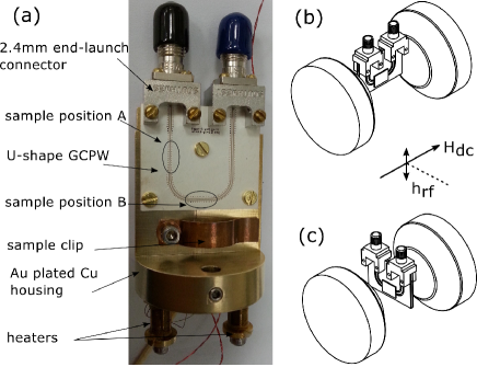
Figure 4: FMR probe-head with u-shape GCPW and end-launch connector. (a) Photograph of the probe-head using end-launch connector and U-shape GCPW. Sensors are mounted at the backside and at the bottom of the Cu housing. Simplified sketch of the configuration for measuring with an external field generated by the split coils (b) parallel and (c) perpendicular to the sample plane. Rotating the dipper probe in the horizontal plane changes from one configuration to the other.

III Experimental test

In this section, we present data to assess the performance of the FMR probe head and discuss two sets of magnetic damping measurements, demonstrating the capabilities and performance of the appratus.

III.1 Spring-loaded sample holder

We tested our setup using a Keysight PNA N5222A vector network analyzer with maximum frequency 26.5 GHz. The output power of the VNA is always 0 dBm in our test. Note that with 2.4 mm connectors and customized GCPW, our design can in principle operate up to 50 GHz. The performance of the spring-loaded sample holder is first studied at room temperature with a 2 nm thick $\textrm{Co}{}_{40}\textrm{Fe}{}_{40}\textrm{B}_{20}$ film. For direct comparison, the FMR spectra are recorded with two sample loading methods: One with a spring-loaded sample holder (Fig. 2) and the other using the common method(Harward et al., 2011) which only requires Kapton tape. The magnetic field is applied parallel to the plane of the thin film sample. Six sets of data were obtained by reloading the sample for each measurement. In Fig. 5, we show the amplitude of the power transmission coefficient from Port 1 to Port 2 (S₂₁) at a frequency of 10 GHz and a temperature of 300 K. The open circles represent a spectrum for a spring-loaded sample mounting whereas the open squares is the spectrum showing largest signal for the six flip-sample loadings. The averaged spectra for all six spectra are shown by solid line and dotted line, for spring and flip-sample loading, respectively. Two observations are evident: First, the best signal we obtained using the flip sample method is approximately 20 percent lower compared to the spring-loaded method. Thus the spring-loaded method gives a better signal to noise ratio and sensitivity. Second, for the spring-loaded method, the difference between the averaged spectrum and single spectra is negligibly small. On the other hand the variation between measurements for the flip-sample method can be as large as 20 percent. Hence the spring-loaded method has better stability and is reproducible.

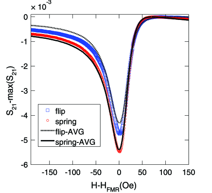
Figure 5: Comparison between S₂₁ signals obtained using spring-loaded sample holder mounting and flip-sample mounting at 300 K. The sample has a stack of MgO(3 nm)—CoFeB(2 nm)—MgO(3 nm) deposited on silicon substrate. (Numbers in parenthesis of the sample composition represent the thickness of the respective layer.) The frequency is 10 GHz and the FMR center field is at 1520 Oe.

III.2 Temperature response

As detailed in the previous section, the probe head is made of Au plated Cu blocks with high internal thermal conduction and good thermal contact. Consequently, the response time of the temperature control will be small as the characteristic thermal relaxation time of a system is $C/k$, where $C$ is the heat capacity and $k$ is the overall thermal conduction. Also, the temperature difference between sample and sensor is minimized even with the heater turned on. Shown in Fig. 6 are the FMR spectra and temperature variation for a CoFeB film of 3 nm thickness measured at 4.4 K. The external field was swept at a rate of about -10 Oe/s. For fields close to which FMR peaks are observed, we detected a temperature rise of a few mK. In fact, the field values corresponding to maximum temperatures are about 20 Oe lower than the fields satisfying FMR condition, showing that the characteristic relaxation time between the sample and cold head is approximately 2 seconds. The temperature rise of the probe head due to FMR indicates that the magnetic system absorbs energy from the microwave and dissipates into the thermal bath. Specifically, at the field satisfying the FMR condition, the damping torque is balanced by the torque generated by the RF field. However, the dissipation power of such process is propotional to the thickness of the magnetic film hence is very small. The successful detection of a temperature rise adds credence to the high thermal conduction within the probe head and relative low thermal conduction between different stages. This demonstration shows that the probe head is capable of measuring samples with phase transitions in a narrow temperature range, such as a superconducting/ferromagnetic bilayer system.(Bell et al., 2008)

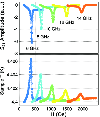
Figure 6: Sample temperature variation due to FMR at selected frequencies. (upper panel) Amplitude of S₂₁ and (lower panel) temperature variation of MgO(3 nm)—CoFeB(3 nm)—MgO(3 nm) at 4.4 K measured with external field parallel to the film plane.

III.3 Magnetic damping measurements

Although the FMR probe can be used to determine the energy anisotropy of magnetic materials, our primary purpose is to study magnetic damping parameter. In the following, two examples of such measurements are briefly described. Shown in Fig. 7 is FMR response of a Py film of 5 nm thickness deposited on a silicon substrate, measured at 4.4 K. The sweeping external magnetic field is parallel to the sample surface. Real and Imaginary parts of the spectra obtained at selected frequencies are plotted with open circles in Fig. 7 (a) and (b), respectively. In FMR measurements, the change in the transmittance, $S_{21}$, is a direct measure of the field-dependent susceptibility of the magnetic layer. According to the Landau–Lifshitz–Gilbert formalism, the dynamic susceptibility of the magnetic material in the configuration where the field is applied parallel to the plane of the thin film be described as:(Bilzer et al., 2006)

$$\chi_{{\rm{\scriptscriptstyle IP}}}=\frac{4\pi M_{{\rm s}}\left(H_{0}+H_{{\rm uni}}+4\pi M_{{\rm eff}}+i\,\Delta H/2\right)}{\left(H_{0}+H_{{\rm uni}}\right)\left(H_{0}+H_{{\rm uni}}+4\pi M_{{\rm eff}}\right)-H_{f}^{2}+i\,(\Delta H/2)\cdot\left[2\left(H_{0}+H_{{\rm uni}}\right)+4\pi M_{{\rm eff}}\right]}$$ (1)

Here, $4\pi M_{{\rm s}}$ is the saturation magnetization, $H_{{\rm uni}}$ is the in-plane uniaxial anisotropy, $4\pi M_{{\rm eff}}$ is the effective magnetization, $H_{f}=2\pi f/\gamma$, and $\Delta H$ is the linewidth of the spectrum – the last term is of key importance to determine the damping parameter. As shown by solid lines in Fig. 7 (a) and (b), the spectra can be fitted very well by adding a background, a drift proportional to time, and a phase factor.(Nembach et al., 2011; Kalarickal et al., 2006) The field linewidth as a function of frequency – $\Delta H\,(f)$ is plotted in Fig. 7 (c). The data points fall on a straight line. The damping parameter $\alpha_{{\rm{\scriptscriptstyle GL}}}=0.012\pm 0.001$ is therefore determined by the slope through(Celinski and Heinrich, 1991; Lenz et al., 2006):

$$\Delta H=\frac{4\pi}{\gamma}\alpha_{{\rm{\scriptscriptstyle GL}}}\,f+\Delta H_{0}$$ (2)

The error bar here is calculated from the confidence interval of the fit.

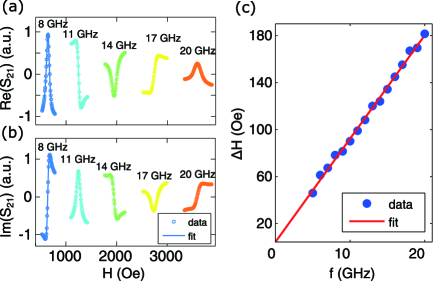
Figure 7: FMR data of a Py thin film of thickness 5 nm measured at 4.4 K with magnetic field applied parallel to the sample plane. (a) Real and (b) Imaginary parts of transmitted signal S₂₁ at selected frequencies. The data are normalized and the relative strength between the spectra at different frequencies are kept. (c) FMR linewidth as a function of frequency. The damping was calculated to be 0.012 $\pm 0.001$, using a linear fit.

We have also tested the setup with a magnetic field applied perpendicular to the sample plane. The results for a MgO (3 nm)—Co₄₀Fe₄₀B₂₀(1.5 nm)—MgO (3nm) stack deposited on silicon substrate are shown in Fig. 8. Comparing the spectra obtained at different temperatures and fixed frequency, two observations are evident. First, the FMR peak position shifts to higher field as the temperature is lowered due to changes in the effective magnetization. Second, the FMR linewidth increases with decreasing temperature. Although the interfacial anisotropy can be determined by fitting the FMR peak positions to the Kittel formula,(Sparks, Loudon, and Kittel, 1961) here, we are more interested in the damping parameter as a function of temperature. The dynamic susceptibility in this configuration is(Devolder et al., 2013):

$$\chi_{{\scriptscriptstyle{\rm OP}}}=\frac{4\pi M_{{\rm s}}\left(H-4\pi M_{{\rm eff}}-i\,\Delta H/2\right)}{\left(H-4\pi M_{{\rm eff}}\right)^{2}-H_{f}^{2}+i\,\Delta H\cdot\left(H-4\pi M_{{\rm eff}}\right)}$$ (3)

Following the same procedure as for Py, the real and imaginary part of the spectra are fitted simultaneously to obtain the linewidth. In Fig. 8 (b), we plot the linewidth as a function of frequency at the two boundaries of our measured temperatures. Although the measured linewidth at lower temperature is larger, the slope of the two curves is in good agreement. The additional linewidth at 6 K is primarily due to zero frequency broadening, which quantifies the magnitude of dispersion of the effective magnetization. The results are summarized in Fig. 8 (c). Gilbert damping is essentially independent of temperature although there is a minimum at 40 K. The room temperature value obtained is in agreement with the value for a thicker CoFeB.(Bilzer et al., 2006; Ikeda et al., 2010) On the other hand, the inhomogeneous broadening increases with lowering temperatue. The value at 6 K is more than double compared to room temperatue. Notably, neglecting the zero-frequency offset $\Delta$H(0), arising due to inhomogeneity, would give rise to an enhanced effective damping compared to the intrinsic contribution. Cavity based, angular dependent FMR may also distinguish the Gilbert damping from inhomogeneity effects. A shortcoming however, is the need to take into account the possible contribution of two magnon scattering, which causes increased complications in the analysis of the data.(Mizukami, Ando, and Miyazaki, 2002; Lindner et al., 2009) On the other hand, broadband FMR using a dipper probe with the applied magnetic field in the perpendicular configuration, rules out two magnon scattering making this technique relatively straightforward to implement.(Arias and Mills, 1999)

The dipper probe discussed here is not limited to measurements of the damping coefficient. The broadband design is also useful for time-domain measurements.(Cui et al., 2010) Furthermore, a spin transfer torque ferromagnetic resonance(Liu et al., 2011) measurement on a single device can be performed with variable temperature using bias Tee and a separate sample holder.

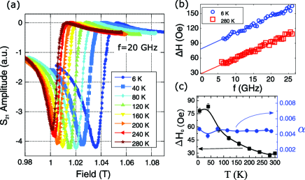
Figure 8: Temperature dependent FMR measurement for a CoFeB thin film of thickness 1.5 nm with the magnetic field applied perpendicular to the film plane. (a) Transmitted FMR signal at 20 GHz obtained at different temperatures. (b) FMR linewidth as a function of frequency at 6 K and 280 K. (c) Damping constant and inhomogeneous broadening as a function of temperature. The solid lines are the guides for the eye.

IV conclusion

We have developed a variable temperature FMR to measure the magnetic damping parameter in ultra thin films. The 3-stage dipper and FMR head with a spring-loaded sample holder design have a temperature stability of milli Kelvin during the FMR measurements. This apparatus demonstrates improved signal stability compared to traditional flip-sample mounting. The results for Py and CoFeB thin films show that the FMR dipper can measure the damping parameter of ultra thin films with: Field parallel and perpendicular to the film plane in the temperature range 4.2-300 K and frequency up to at least 26 GHz.