Uniform error bounds of a finite difference method for the Zakharov system in the subsonic limit regime via an asymptotic consistent formulation

Abstract

We present a uniformly accurate finite difference method and establish rigorously its uniform error bounds for the Zakharov system (ZS) with a dimensionless parameter $0<\varepsilon\leq 1$, which is inversely proportional to the speed of sound. In the subsonic limit regime, i.e., $0<\varepsilon\ll 1$, the solution propagates highly oscillatory waves and/or rapid outgoing initial layers due to the perturbation of the wave operator in ZS and/or the incompatibility of the initial data which is characterized by two nonnegative parameters $\alpha$ and $\beta$. Specifically, the solution propagates waves with $O(\varepsilon)$- and $O(1)$-wavelength in time and space, respectively, and amplitude at $O(\varepsilon^{\min\{2,\alpha,1+\beta\}})$ and $O(\varepsilon^{\alpha})$ for well-prepared ($\alpha\geq 1$) and ill-prepared ($0\leq\alpha<1$) initial data, respectively. This high oscillation of the solution in time brings significant difficulties in designing numerical methods and establishing their error bounds, especially in the subsonic limit regime. A uniformly accurate finite difference method is proposed by reformulating ZS into an asymptotic consistent formulation and adopting an integral approximation of the oscillatory term. By adapting the energy method and using the limiting equation via a nonlinear Schrödinger equation with an oscillatory potential, we rigorously establish two independent error bounds at $O(h^{2}+\tau^{2}/\varepsilon)$ and $O(h^{2}+\tau^{2}+\tau\varepsilon^{\alpha^{*}}+\varepsilon^{1+\alpha^{*}})$, respectively, with $h$ the mesh size, $\tau$ the time step and $\alpha^{*}=\min\{1,\alpha\}$. Thus we obtain error bounds at $O(h^{2}+\tau^{4/3})$ and $O(h^{2}+\tau^{1+\frac{\alpha}{2+\alpha}})$ for well-prepared and ill-prepared initial data, respectively, which are uniform in both space and time for $0<\varepsilon\leq 1$ and optimal at the second order in space. Other techniques in the analysis include the cut-off technique for treating the nonlinearity and inverse estimates to bound the numerical solution. Numerical results are reported to demonstrate that our error bounds are sharp.

1 Introduction

Consider the dimensionless Zakharov system (ZS) for describing the propagation of Langmuir waves in plasma [30, 27]

(1.1) $$\begin{split}&i\partial_{t}E^{\varepsilon}({\bf x},t)+\Delta E^{\varepsilon}({\bf x},t)-N^{\varepsilon}({\bf x},t)E^{\varepsilon}({\bf x},t)=0,\quad{\bf x}\in\mathbb{R}^{d},\quad t>0,\\ &\varepsilon^{2}\partial_{tt}N^{\varepsilon}({\bf x},t)-\Delta N^{\varepsilon}({\bf x},t)-\Delta|E^{\varepsilon}({\bf x},t)|^{2}=0,\quad{\bf x}\in\mathbb{R}^{d},\quad t>0,\\ &E^{\varepsilon}({\bf x},0)=E_{0}({\bf x}),\quad N^{\varepsilon}({\bf x},0)=N_{0}^{\varepsilon}({\bf x}),\quad\partial_{t}N^{\varepsilon}({\bf x},0)=N_{1}^{\varepsilon}({\bf x}),\quad{\bf x}\in\mathbb{R}^{d}.\end{split}$$

Here $t$ is time, ${\bf x}$ is the spatial coordinates, the complex function $E^{\varepsilon}:=E^{\varepsilon}({\bf x},t)$ is the slowly varying envelope of the highly oscillatory electric field, the real function $N^{\varepsilon}:=N^{\varepsilon}({\bf x},t)$ represents the deviation of the ion density from its equilibrium value, $0<\varepsilon\leq 1$ is a dimensionless parameter which is inversely proportional to the acoustic speed, and $E_{0}({\bf x})$, $N_{0}^{\varepsilon}({\bf x})$ and $N_{1}^{\varepsilon}({\bf x})$ are given functions satisfying $\int_{\mathbb{R}^{d}}N_{1}^{\varepsilon}({\bf x})d{\bf x}=0$.

There exist extensive analytical and numerical studies in the literatures for the standard ZS, i.e. $\varepsilon=1$ in (1.1). Along the analytical part, for the derivation of ZS from the Euler-Poisson equations, we refer to [18, 30]; and for the well-posedness, we refer to [12, 16, 18, 30] and references therein. Based on these results, we know that the ZS (1.1) conserves the wave energy

(1.2) $$\mathcal{M}(t)=\|E^{\varepsilon}(\cdot,t)\|^{2}:=\int_{\mathbb{R}^{d}}|E^{\varepsilon}({\bf x},t)|^{2}d{\bf x}\equiv\int_{\mathbb{R}^{d}}|E_{0}({\bf x})|^{2}d{\bf x}=\mathcal{M}(0),\quad t\geq 0,$$

and the Hamiltonian

(1.3) $$\mathcal{L}^{\varepsilon}(t):=\int_{\mathbb{R}^{d}}\left[|\nabla E^{\varepsilon}|^{2}+N^{\varepsilon}|E^{\varepsilon}|^{2}+\frac{1}{2}\left(\varepsilon^{2}|\nabla U^{\varepsilon}|^{2}+|N^{\varepsilon}|^{2}\right)\right]d{\bf x}\equiv\mathcal{L}^{\varepsilon}(0),\quad t\geq 0,$$

where $U^{\varepsilon}:=U^{\varepsilon}({\bf x},t)$ is defined as

(1.4) $$-\Delta U^{\varepsilon}({\bf x},t)=\partial_{t}N^{\varepsilon}({\bf x},t),\quad{\bf x}\in\mathbb{R}^{d},\qquad\lim\limits_{|{\bf x}|\rightarrow\infty}U^{\varepsilon}({\bf x},t)=0,\qquad t\geq 0.$$

Along the numerical part, different numerical methods have been proposed and analyzed in the last two decades. Glassey [19] presented an energy-preserving implicit finite difference scheme and established an error bound at first order in both spatial and temporal discretizations. Later, Chang and Jiang [14] improved it to the optimal second order convergence by considering an implicit or semi-explicit conservative finite difference schemes [15]. Other approaches include the exponential-wave-integrator spectral method [9, 28], Jacobi-type method [11], Legendre-Galerkin method [22], discontinuous-Galerkin method [33] and time-splitting spectral method [8, 24]. The analytical and numerical results for ZS have been extended to the generalized Zakharov system [20, 21], the vector Zakharov system [31] and the vector Zakharov system for multicomponents [21].

When $\varepsilon\to 0^{+}$, i.e., in the subsonic limit regime, formally we get $E^{\varepsilon}({\bf x},t)\to E({\bf x},t)$, $\rho^{\varepsilon}:=\rho^{\varepsilon}({\bf x},t)=|E^{\varepsilon}|^{2}\to|E|^{2}=\rho$ and $N^{\varepsilon}({\bf x},t)\to N({\bf x},t)=-|E({\bf x},t)|^{2}$, where $E:=E({\bf x},t)$ satisfies the cubic nonlinear Schrödinger equation (NLSE) [26, 27, 29]

(1.5) $$\begin{split}&i\partial_{t}E({\bf x},t)+\Delta E({\bf x},t)+|E({\bf x},t)|^{2}E({\bf x},t)=0,\quad t>0,\quad{\bf x}\in\mathbb{R}^{d},\\ &E({\bf x},0)=E_{0}({\bf x}),\quad{\bf x}\in\mathbb{R}^{d}.\end{split}$$

The NLSE (1.5) conserves the wave energy (1.2) with $E^{\varepsilon}=E$ and the Hamiltonian

(1.6) $$\mathcal{L}(t):=\int_{\mathbb{R}^{d}}\left[|\nabla E({\bf x},t)|^{2}-\frac{1}{2}|E({\bf x},t)|^{4}\right]d{\bf x}\equiv\mathcal{L}(0),\quad t\geq 0.$$

Convergence rates of the subsonic limit from the ZS (1.1) to the NLSE (1.5) and initial layers as well as the propagation of oscillatory waves have been rigorously studied in the literatures [26, 27, 29]. Based on the results, when $0<\varepsilon\ll 1$, the solution of the ZS (1.1) propagates highly oscillatory waves at wavelength $O(\varepsilon)$ and $O(1)$ in time and space, respectively, and/or rapid outgoing initial layers at speed $O(1/\varepsilon)$ in space. In addition, the initial data ($E_{0},N_{0}^{\varepsilon},N_{1}^{\varepsilon}$) in (1.1) can be decomposed as

(1.7) $$\begin{split}&\qquad\ N_{0}^{\varepsilon}({\bf x})=N({\bf x},0)+\varepsilon^{\alpha}\omega_{0}({\bf x}),\quad N_{1}^{\varepsilon}({\bf x})=\partial_{t}N({\bf x},0)+\varepsilon^{\beta}\omega_{1}({\bf x}),\qquad{\bf x}\in\mathbb{R}^{d},\\ &\qquad\ N({\bf x},0)=-|E_{0}({\bf x})|^{2},\quad\partial_{t}N({\bf x},0)=-\partial_{t}\rho({\bf x},0)=2\mathrm{Im}(\Delta E_{0}({\bf x})\overline{E_{0}({\bf x})}):=\phi_{1}({\bf x}),\end{split}$$

where $\alpha,\beta\geq 0$ are parameters describing the incompatibility of the initial data of the ZS (1.1) with respect to that of the NLSE (1.5) in the subsonic limit regime, $\omega_{0}({\bf x})$ and $\omega_{1}({\bf x})$ are two given real functions independent of $\varepsilon$ and satisfy $\int_{\mathbb{R}^{d}}\omega_{1}({\bf x})d{\bf x}=0$, and $\mathrm{Im}(f)$ and $\overline{f}$ denote the imaginary and complex conjugate parts of $f$, respectively. In fact, when $\alpha\geq 2$ and $\beta\geq 1$, the leading order oscillation is due to the term $\varepsilon^{2}\partial_{tt}N$ in ZS; and when either $0\leq\alpha<2$ or $0\leq\beta<1$, the leading order oscillation is due to the initial data.

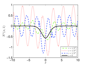
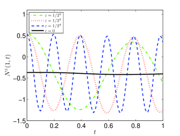
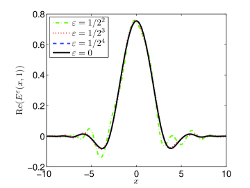
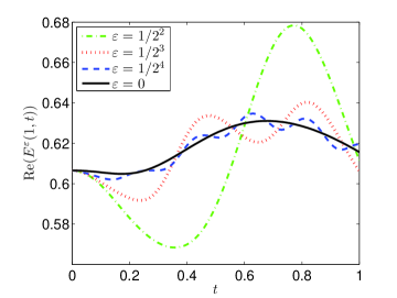
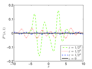
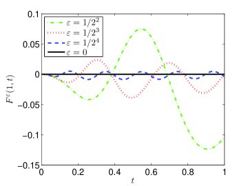
Fig. 1: The solutions of the ZS (1.1) for different $\varepsilon>0$ and the NLSE ($\varepsilon=0$) as well as $F^{\varepsilon}$ defined in (2.8) with $d=1$. Here $\mathrm{Re}(f)$ denotes the real part of $f$.

To illustrate the oscillatory and/or rapid outgoing wave phenomena, Fig. 1 shows the solutions $N^{\varepsilon}(x,1)$, $N^{\varepsilon}(1,t)$, Re$(E^{\varepsilon}(x,1))$ and Re$(E^{\varepsilon}(1,t))$ of the ZS (1.1) with $d=1$, $E_{0}(x)=e^{-x^{2}/2}$, $\alpha=0$, $\beta=0$, $\omega_{0}(x)=e^{-\frac{1}{18^{2}-x^{2}}}\sin(2x)\chi_{(-18,18)}$ with $\chi$ the characteristic function and $\omega_{1}(x)\equiv 0$ in (1.7) for different $\varepsilon$, which was obtained numerically on a bounded computational interval $[-200,200]$ with the homogenous Dirichlet boundary condition [8]. For comparison, here we also plot $F^{\varepsilon}(x,1)$ and $F^{\varepsilon}(1,t)$ defined in (2.8).

The highly oscillatory nature of the solution of the ZS (1.1) in time brings significant numerical burdens, especially in the subsonic limit regime. Some numerical results for ZS with different $0<\varepsilon\leq 1$ have been reported in the literatures [8, 24]. To the best of our knowledge, there are few results concerning error estimates of different numerical methods for ZS with respect to the mesh size $h$, time step $\tau$ as well as the parameter $0<\varepsilon\leq 1$ except that an error bound of the finite difference Legendre pseduospectral method was derived for ZS in one dimension (1D) when $\alpha\geq 2$ and $\beta\geq 1$ [22]. Very recently, for the conservative finite difference method, Cai and Yuan [13] established uniform error bounds at $O(h^{2}+\tau^{4/3})$ for $0<\varepsilon\leq 1$ when $\alpha\geq 2$ and $\beta\geq 1$, and at $O(h^{2}+\tau^{\frac{2}{3}\min\{\alpha,1+\beta\}})$ when $1\leq\alpha<2$ and/or $0\leq\beta<1$. However, when $0<\alpha<1$, their error bound $O(h^{2}/\varepsilon^{1-\alpha}+\tau^{\frac{2}{3}\alpha})$ is not uniform in space, and in particular, when $\alpha=0$, their error bound $O(h^{2}/\varepsilon+\tau^{2}/\varepsilon^{3})$ requests the meshing strategy (or $\varepsilon$-scalability) $h=O(\varepsilon^{1/2})$ and $\tau=O(\varepsilon^{3/2})$ which is not uniform in both space and time when $0<\varepsilon\ll 1$. The reason is due to that $N^{\varepsilon}({\bf x},t)$ does not converge to $N({\bf x},t)=-|E({\bf x},t)|^{2}$ when $\alpha=0$ and $\varepsilon\to 0^{+}$ [26, 29, 31] (cf. Fig 1.1 top row).

The aim of this work is to design a finite difference method for ZS, which is uniformly accurate in space and time for $0<\varepsilon\leq 1$, and carry out rigorous error analysis for the finite difference method by paying particular attention to how the error bounds depend on explicitly $h$ and $\tau$ as well as the parameter $\varepsilon$. The key ingredients in designing the uniformly accurate finite difference method are based on (i) reformulating ZS into an asymptotic consistent formulation and (ii) adapting an integral approximation of the oscillatory term. In establishing error bounds, we adapt the energy method, cut-off technique for treating the nonlinearity, the inverse estimates to bound the numerical solution, and the limiting equation via a nonlinear Schrödinger equation with an oscillatory potential. The error bounds of our new numerical method significantly improve the results of the standard finite difference method for ZS in the subsonic limit regime [13], especially for the ill-prepared initial data, i.e. $0\leq\alpha<1$.

The rest of the paper is organized as follows. In section 2, we introduce an asymptotic consistent formulation of ZS, present a finite difference method and state our main results. Section 3 is devoted to the details of the error analysis. Numerical results are reported in section 4 to confirm our error bounds. Finally some conclusions are drawn in section 5. Throughout the paper, we adopt the standard Sobolev spaces and the corresponding norms and adopt $A\lesssim B$ to mean that there exists a generic constant $C>0$ independent of $\varepsilon$, $\tau$, $h$, such that $|A|\leq C\,B$.

2 A finite difference method and its error bounds

In this section, we will introduce an asymptotic consistent formulation of ZS, present a uniformly accurate finite difference method and state its error bounds.

2.1 An asymptotic consistent formulation

Introduce

(2.8) $$F^{\varepsilon}({\bf x},t)=N^{\varepsilon}({\bf x},t)+|E^{\varepsilon}({\bf x},t)|^{2}-G^{\varepsilon}({\bf x},t/\varepsilon),\qquad{\bf x}\in\mathbb{R}^{d},\quad t\geq 0,$$

where

(2.9) $$G^{\varepsilon}({\bf x},s)=\varepsilon^{\alpha}G_{1}({\bf x},s)+\varepsilon^{1+\beta}G_{2}({\bf x},s),\qquad{\bf x}\in\mathbb{R}^{d},\quad s\geq 0,$$

with $G_{j}({\bf x},s)$ ($j=1,2$) being the solutions of the linear wave equations

(2.10) $$\begin{split}&\partial_{ss}G_{j}({\bf x},s)-\Delta G_{j}({\bf x},s)=0,\qquad{\bf x}\in\mathbb{R}^{d},\quad s>0,\\ &G_{1}({\bf x},0)=\omega_{0}({\bf x}),\quad\partial_{s}G_{1}({\bf x},0)\equiv 0,\quad G_{2}({\bf x},0)\equiv 0,\quad\partial_{s}G_{2}({\bf x},0)=\omega_{1}({\bf x}).\end{split}$$

Plugging (2.8) into the ZS (1.1), we can reformulate it into an asymptotic consistent formulation

(2.11) $$\begin{split}&i\partial_{t}E^{\varepsilon}({\bf x},t)+\Delta E^{\varepsilon}({\bf x},t)+\left[|E^{\varepsilon}({\bf x},t)|^{2}-F^{\varepsilon}({\bf x},t)-G^{\varepsilon}({\bf x},t/\varepsilon)\right]E^{\varepsilon}({\bf x},t)=0,\\ &\varepsilon^{2}\partial_{tt}F^{\varepsilon}({\bf x},t)-\Delta F^{\varepsilon}({\bf x},t)-\varepsilon^{2}\partial_{tt}|E^{\varepsilon}({\bf x},t)|^{2}=0,\quad{\bf x}\in\mathbb{R}^{d},\quad t>0,\\ &E^{\varepsilon}({\bf x},0)=E_{0}({\bf x}),\quad F^{\varepsilon}({\bf x},0)\equiv 0,\quad\partial_{t}F^{\varepsilon}({\bf x},0)\equiv 0,\quad{\bf x}\in\mathbb{R}^{d}.\end{split}$$

Now the initial conditions in (2.11) are always well-prepared for any $\alpha\geq 0$ and $\beta\geq 0$. In addition, the above system conserves the wave energy (1.2) and the ‘modified’ Hamiltonian

(2.12) $$\widetilde{\mathcal{L}}^{\varepsilon}(t) := \int_{\mathbb{R}^{d}}\biggl{[}|\nabla E^{\varepsilon}|^{2}-\frac{1}{2}|E^{\varepsilon}|^{4}+\frac{1}{2}|F^{\varepsilon}|^{2}+\frac{1}{\varepsilon^{2}}\int_{0}^{t}\int_{0}^{s}\nabla F^{\varepsilon}({\bf x},s)\cdot\nabla F^{\varepsilon}({\bf x},s^{\prime})ds^{\prime}ds$$

$$+\int_{0}^{t}\left[G({\bf x},s/\varepsilon)\partial_{s}|E^{\varepsilon}({\bf x},s)|^{2}-\phi_{1}({\bf x})F^{\varepsilon}({\bf x},s)\right]ds\biggr{]}d{\bf x}\equiv\widetilde{\mathcal{L}}^{\varepsilon}(0),\quad t\geq 0.$$

When $\varepsilon\to 0^{+}$, i.e., in the subsonic limit regime, formally we get $E^{\varepsilon}({\bf x},t)\to E({\bf x},t)$ and $F^{\varepsilon}({\bf x},t)\to 0$, where $E:=E({\bf x},t)$ satisfies the NLSE (1.5). In addition, when $\varepsilon\to 0^{+}$, formally we can also get $E^{\varepsilon}({\bf x},t)\to\widetilde{E}^{\varepsilon}({\bf x},t)$ and $F^{\varepsilon}({\bf x},t)\to 0$, where $\widetilde{E}^{\varepsilon}:=\widetilde{E}^{\varepsilon}({\bf x},t)$ satisfies the following nonlinear Schrödinger equation with an oscillatory potential $G^{\varepsilon}({\bf x},t/\varepsilon)$ (NLSE-OP)

(2.13) $$\begin{split}&i\partial_{t}\widetilde{E}^{\varepsilon}({\bf x},t)+\Delta\widetilde{E}^{\varepsilon}({\bf x},t)+\left[|\widetilde{E}^{\varepsilon}({\bf x},t)|^{2}-G^{\varepsilon}({\bf x},t/\varepsilon)\right]\widetilde{E}^{\varepsilon}({\bf x},t)=0,\qquad t>0,\\ &\widetilde{E}^{\varepsilon}({\bf x},0)=E_{0}({\bf x}),\quad{\bf x}\in\mathbb{R}^{d}.\end{split}$$

It conserves the wave energy (1.2) with $E^{\varepsilon}=\widetilde{E}^{\varepsilon}$ and the ‘modified’ Hamiltonian

(2.14) $$\qquad\ \widetilde{{\mathcal{L}}}(t):=\int_{\mathbb{R}^{d}}\left[|\nabla\widetilde{E}^{\varepsilon}|^{2}-\frac{1}{2}|\widetilde{E}^{\varepsilon}|^{4}+\int_{0}^{t}G({\bf x},\frac{s}{\varepsilon})\partial_{s}|\widetilde{E}^{\varepsilon}({\bf x},s)|^{2}ds\right]d{\bf x}\equiv\widetilde{{\mathcal{L}}}(0),\ t\geq 0.$$

2.2 A uniformly accurate finite difference method

For simplicity of notations, we will only present the numerical method for the ZS (2.11) in 1D and extensions to higher dimensions are straightforward. When $d=1$, we truncate ZS on a bounded computational interval $\Omega=(a,b)$ with homogeneous Dirichlet boundary condition (here $|a|$ and $b$ are chosen large enough such that the truncation error is negligible):

(2.15) $$\begin{split}&i\partial_{t}E^{\varepsilon}(x,t)+\partial_{xx}E^{\varepsilon}(x,t)+[|E^{\varepsilon}(x,t)|^{2}-F^{\varepsilon}(x,t)-G^{\varepsilon}(x,t/\varepsilon)]E^{\varepsilon}(x,t)=0,\\ &\varepsilon^{2}\partial_{tt}F^{\varepsilon}(x,t)-\partial_{xx}F^{\varepsilon}(x,t)-\varepsilon^{2}\partial_{tt}|E^{\varepsilon}(x,t)|^{2}=0,\quad x\in\Omega,\quad t>0,\\ &E^{\varepsilon}(x,0)=E_{0}(x),\quad F^{\varepsilon}(x,0)\equiv 0,\quad\partial_{t}F^{\varepsilon}(x,0)\equiv 0,\quad x\in\bar{\Omega},\\ &E^{\varepsilon}(a,t)=E^{\varepsilon}(b,t)=0,\qquad F^{\varepsilon}(a,t)=F^{\varepsilon}(b,t)=0,\qquad t\geq 0,\end{split}$$

where $G^{\varepsilon}(x,s)$ is defined as (2.9) with $d=1$ and $G_{j}(x,s)$ ($j=1,2$) being the solutions of the wave equations

(2.16) $$\begin{split}&\partial_{ss}G_{j}(x,s)-\partial_{xx}G_{j}(x,s)=0,\qquad x\in\Omega,\quad s>0,\\ &G_{1}(x,0)=\omega_{0}(x),\quad\partial_{s}G_{1}(x,0)\equiv 0,\quad G_{2}(x,0)\equiv 0,\quad\partial_{s}G_{2}(x,0)=\omega_{1}(x),\\ &G_{1}(a,s)=G_{1}(b,s)=G_{2}(a,s)=G_{2}(b,s)=0,\qquad s\geq 0.\end{split}$$

When $\varepsilon\to 0^{+}$, formally we get $E^{\varepsilon}(x,t)\to\widetilde{E}^{\varepsilon}(x,t)$ and $F^{\varepsilon}(x,t)\to 0$, where $\widetilde{E}^{\varepsilon}:=\widetilde{E}^{\varepsilon}(x,t)$ satisfies the NLSE-OP

(2.17) $$\begin{split}&\qquad i\partial_{t}\widetilde{E}^{\varepsilon}(x,t)+\partial_{xx}\widetilde{E}^{\varepsilon}(x,t)+\left[|\widetilde{E}^{\varepsilon}(x,t)|^{2}-G^{\varepsilon}(x,t/\varepsilon)\right]\widetilde{E}^{\varepsilon}(x,t)=0,\ \ t>0,\\ &\qquad\widetilde{E}^{\varepsilon}(x,0)=E_{0}(x),\quad{\bf x}\in\bar{\Omega};\qquad\widetilde{E}^{\varepsilon}(a,t)=\widetilde{E}^{\varepsilon}(b,t)=0,\quad t\geq 0.\end{split}$$

Choose a mesh size $h:=\Delta x=(b-a)/M$ with $M$ being a positive integer and a time step $\tau:=\Delta t>0$ and denote the grid points and time steps as

$$x_{j}:=a+jh,\quad j=0,1,\cdots,M;\quad t_{k}:=k\tau,\quad k=0,1,2,\cdots.$$

Define the index sets

$$\mathcal{T}_{M}=\{j\ |\ j=1,2,\cdots,M-1\},\quad\mathcal{T}_{M}^{0}=\{j\ |\ j=0,1,\cdots,M\}.$$

Let $E^{\varepsilon,k}_{j}$ and $F^{\varepsilon,k}_{j}$ be the approximations of $E^{\varepsilon}(x_{j},t_{k})$ and $F^{\varepsilon}(x_{j},t_{k})$, respectively, and denote $E^{\varepsilon,k}=(E^{\varepsilon,k}_{0},E^{\varepsilon,k}_{1},\ldots,E^{\varepsilon,k}_{M})^{T}\in\mathbb{C}^{(M+1)}$, $F^{\varepsilon,k}=(F^{\varepsilon,k}_{0},F^{\varepsilon,k}_{1},\ldots,F^{\varepsilon,k}_{M})^{T}\in\mathbb{R}^{(M+1)}$ as the numerical solution vectors at $t=t_{k}$. Define the standard finite difference operators

$$\delta_{t}^{+}E_{j}^{k}=\frac{E_{j}^{k+1}-E_{j}^{k}}{\tau},\quad\delta_{t}E_{j}^{k}=\frac{E_{j}^{k+1}-E_{j}^{k-1}}{2\tau},\quad\delta_{t}^{2}E_{j}^{k}=\frac{E_{j}^{k+1}-2E_{j}^{k}+E_{j}^{k-1}}{\tau^{2}},$$

$$\delta_{x}^{+}E_{j}^{k}=\frac{E_{j+1}^{k}-E_{j}^{k}}{h},\qquad\delta_{x}^{2}E_{j}^{k}=\frac{E_{j+1}^{k}-2E_{j}^{k}+E_{j-1}^{k}}{h^{2}}.$$

We present a finite difference discretization of (2.15) as following

(2.18) $$i\delta_{t}E_{j}^{\varepsilon,k}=\left(-\delta_{x}^{2}-|E_{j}^{\varepsilon,k}|^{2}+H_{j}^{\varepsilon,k}+\frac{F_{j}^{\varepsilon,k+1}+F_{j}^{\varepsilon,k-1}}{2}\right)\frac{E_{j}^{\varepsilon,k+1}+E_{j}^{\varepsilon,k-1}}{2},$$

$$\varepsilon^{2}\delta_{t}^{2}F_{j}^{\varepsilon,k}=\frac{1}{2}\delta_{x}^{2}(F_{j}^{\varepsilon,k+1}+F_{j}^{\varepsilon,k-1})+\varepsilon^{2}\delta_{t}^{2}|E_{j}^{\varepsilon,k}|^{2},\quad j\in\mathcal{T}_{M},\quad k\geq 1,$$

where an average of the oscillatory potential $G^{\varepsilon}$ over the interval $[t_{k-1},t_{k+1}]$ is used

(2.19) $$\qquad\ \ H_{j}^{\varepsilon,k}=\frac{1}{2\tau}\int_{t_{k-1}}^{t_{k+1}}G^{\varepsilon}(x_{j},s/\varepsilon)ds=\frac{\varepsilon}{2\tau}\int_{t_{k-1}/\varepsilon}^{t_{k+1}/\varepsilon}G^{\varepsilon}(x_{j},u)du,\quad j\in\mathcal{T}_{M},\quad k\geq 1.$$

The boundary and initial conditions are discretized as

(2.20) $$\qquad\ \ E_{0}^{\varepsilon,k}=E_{M}^{\varepsilon,k}=F_{0}^{\varepsilon,k}=F_{M}^{\varepsilon,k}=0,\ k\geq 0;\quad E_{j}^{\varepsilon,0}=E_{0}(x_{j}),\ F_{j}^{\varepsilon,0}=0,\quad j\in\mathcal{T}_{M}^{0}.$$

In addition, the first step $E_{j}^{\varepsilon,1}$ and $F_{j}^{\varepsilon,1}$ can be obtained via (2.15) and the Taylor expansion as

(2.21) $$E_{j}^{\varepsilon,1}=E_{0}(x_{j})+\tau\phi_{2}(x_{j})+\frac{\tau^{2}}{2}\phi_{3}(x_{j}),\quad F_{j}^{\varepsilon,1}=\frac{\tau^{2}}{2}\phi_{4}(x_{j}),\quad j\in\mathcal{T}_{M},$$

where

(2.22) $$\begin{split}&\phi_{2}(x):=\partial_{t}E^{\varepsilon}(x,0)=i\left[E_{0}^{\prime\prime}(x)-N_{0}^{\varepsilon}(x)E_{0}(x)\right],\\ &\phi_{3}(x):=\partial_{tt}E^{\varepsilon}(x,0)=i\left[\phi_{2}^{\prime\prime}(x)-N_{1}^{\varepsilon}(x)E_{0}(x)-N_{0}^{\varepsilon}(x)\phi_{2}(x)\right],\qquad x\in\Omega,\\ &\phi_{4}(x):=\partial_{tt}F^{\varepsilon}(x,0)=\partial_{tt}\rho^{\varepsilon}(x,0)=2{\rm Im}\left[\phi_{2}(x)\overline{E_{0}^{\prime\prime}(x)}+E_{0}(x)\overline{\phi_{2}^{\prime\prime}(x)}\right].\end{split}$$

If it is needed in practical computation, the second order derivatives in (2.22) can be approximated by the second order finite difference as $f^{\prime\prime}(x_{j})\approx\delta_{x}^{2}f(x_{j})$ for $j\in\mathcal{T}_{M}$. In addition, $H_{j}^{\varepsilon,k}$ in (2.19) can be approximated by solving the wave equations (2.16) via the sine pseudospectral method in space and then integrating in time in phase space exactly as

$$H_{j}^{\varepsilon,k} \approx \frac{\varepsilon}{2\tau}\sum_{l=1}^{M-1}\sin\left(\mu_{l}(x_{j}-a)\right)\int_{t_{k-1}/\varepsilon}^{t_{k+1}/\varepsilon}\left[\varepsilon^{\alpha}\widetilde{(\omega_{0})}_{l}\cos(\mu_{l}u)+\frac{\varepsilon^{1+\beta}}{\mu_{l}}\widetilde{(\omega_{1})}_{l}\sin(\mu_{l}u)\right]du$$

$$= \sum_{l=1}^{M-1}\frac{\varepsilon}{\tau\mu_{l}}\sin\left(\frac{lj\pi}{M}\right)\sin\left(\frac{\tau\mu_{l}}{\varepsilon}\right)\left[\varepsilon^{\alpha}\widetilde{(\omega_{0})}_{l}\cos\left(\frac{\mu_{l}t_{k}}{\varepsilon}\right)+\frac{\varepsilon^{1+\beta}}{\mu_{l}}\widetilde{(\omega_{1})}_{l}\sin\left(\frac{\mu_{l}t_{k}}{\varepsilon}\right)\right],$$

where for $l=1,2,\ldots,M-1$,

$$\mu_{l}=\frac{l\pi}{b-a},\quad\widetilde{(\omega_{0})}_{l}=\frac{2}{M}\sum_{j=1}^{M-1}\omega_{0}(x_{j})\sin\left(\frac{lj\pi}{M}\right),\quad\widetilde{(\omega_{1})}_{l}=\frac{2}{M}\sum_{j=1}^{M-1}\omega_{1}(x_{j})\sin\left(\frac{lj\pi}{M}\right).$$

2.3 Main results

For convenience of notation, denote

$$0\leq\alpha^{*}=\min\{\alpha,1\}\leq 1.$$

Let $T^{*}>0$ be the maximum common existence time for the solutions of the ZS (2.15) and the NLSE-OP (2.17). Then for any fixed $0<T<T^{*}$, according to the known results in [1, 26, 27, 29], we assume that the solution $(E^{\varepsilon},F^{\varepsilon})$ of the ZS (2.15) and the solution $\widetilde{E}^{\varepsilon}$ of the NLSE-OP (2.17) are smooth enough over $\Omega_{T}:=\Omega\times[0,T]$ and satisfy

$$(A)\begin{split}&\|E^{\varepsilon}\|_{W^{5,\infty}}+\|\partial_{t}E^{\varepsilon}\|_{W^{1,\infty}}+\|\partial_{tt}F^{\varepsilon}\|_{W^{2,\infty}}+\|\widetilde{E}^{\varepsilon}\|_{W^{5,\infty}}+\|\partial_{t}\widetilde{E}^{\varepsilon}\|_{W^{1,\infty}}\lesssim 1,\\ &\|F^{\varepsilon}\|_{W^{4,\infty}}\lesssim\varepsilon^{2},\qquad\|\partial_{t}F^{\varepsilon}\|_{W^{4,\infty}}\lesssim\varepsilon,\qquad\|\partial_{tt}\widetilde{E}^{\varepsilon}\|_{W^{4,\infty}}\lesssim\frac{1}{\varepsilon^{1-\alpha^{*}}},\\ &\|\partial_{tt}E^{\varepsilon}\|_{W^{4,\infty}}+\|\partial_{t}^{3}F^{\varepsilon}\|_{W^{2,\infty}}\lesssim\frac{1}{\varepsilon},\qquad\|\partial_{t}^{3}E^{\varepsilon}\|_{W^{4,\infty}}+\|\partial_{t}^{4}F^{\varepsilon}\|_{W^{2,\infty}}\lesssim\frac{1}{\varepsilon^{2}}.\end{split}$$

We further assume that the initial data satisfy

$$(B)\hskip 85.35826pt\|E_{0}\|_{W^{5,\infty}(\Omega)}+\|\omega_{0}\|_{W^{3,\infty}(\Omega)}+\|\omega_{1}\|_{W^{3,\infty}(\Omega)}\lesssim 1.\hskip 170.71652pt$$

Then one can obtain [26, 29, 31]

(2.23) $$\|G^{\varepsilon}\|_{W^{3,\infty}([0,\infty),W^{3,\infty}(\Omega))}\lesssim\varepsilon^{\alpha^{*}}.$$

In addition, we assume the following convergence rate from ZS to NLSE-OP

$$(C)\hskip 85.35826pt\|E^{\varepsilon}-\widetilde{E}^{\varepsilon}\|_{L^{\infty}([0,T];H^{1}(\Omega))}\lesssim\varepsilon^{2}.\hskip 170.71652pt$$

Denote

$$X_{M}=\left\{v=\left(v_{0},v_{1},\ldots,v_{M}\right)^{T}\ |\ v_{0}=v_{M}=0\right\}\subseteq\mathbb{C}^{M+1},$$

equipped with norms and inner products defined as

$$\|u\|^{2}=h\sum\limits_{j=1}^{M-1}|u_{j}|^{2},\quad\|\delta_{x}^{+}u\|^{2}=h\sum\limits_{j=0}^{M-1}|\delta_{x}^{+}u_{j}|^{2},\quad\|u\|_{\infty}=\sup\limits_{j\in\mathcal{T}_{M}^{0}}|u_{j}|,$$

$$(u,v)=h\sum\limits_{j=1}^{M-1}u_{j}\overline{v_{j}},\quad\langle\delta_{x}^{+}u,\delta_{x}^{+}v\rangle=h\sum\limits_{j=0}^{M-1}(\delta_{x}^{+}u_{j})\;(\delta_{x}^{+}\overline{v_{j}}),\qquad u,v\in X_{M}.$$

Then we have

(2.24) $$(-\delta_{x}^{2}u,v)=\langle\delta_{x}^{+}u,\delta_{x}^{+}v\rangle,\quad((-\delta_{x}^{2})^{-1}u,v)=(u,(-\delta_{x}^{2})^{-1}v),\qquad u,v\in X_{M}.$$

Define the error functions $e^{\varepsilon,k}\in X_{M}$ and $f^{\varepsilon,k}\in X_{M}$ as

(2.25) $$e^{\varepsilon,k}_{j}=E^{\varepsilon}(x_{j},t_{k})-E_{j}^{\varepsilon,k},\quad f_{j}^{\varepsilon,k}=F^{\varepsilon}(x_{j},t_{k})-F_{j}^{\varepsilon,k},\quad j\in\mathcal{T}_{M}^{0},\quad 0\leq k\leq\frac{T}{\tau}.$$

Then we have the following error estimates for (2.18) with (2.19)-(2.21).

Theorem 1.

Under the assumptions (A)-(C), there exist $h_{0}>0$ and $\tau_{0}>0$ sufficiently small and independent of $0<\varepsilon\leq 1$ such that, when $0<h\leq h_{0}$ and $0<\tau\leq\tau_{0}$, the following two error estimates of the scheme (2.18) with (2.19)-(2.21) hold

(2.26) $$\|e^{\varepsilon,k}\|+\|\delta_{x}^{+}e^{\varepsilon,k}\|+\|f^{\varepsilon,k}\| \lesssim h^{2}+\frac{\tau^{2}}{\varepsilon},\qquad 0\leq k\leq\frac{T}{\tau},\quad 0<\varepsilon\leq 1,$$

(2.27) $$\|e^{\varepsilon,k}\|+\|\delta_{x}^{+}e^{\varepsilon,k}\|+\|f^{\varepsilon,k}\| \lesssim h^{2}+\tau^{2}+\tau\varepsilon^{\alpha^{*}}+\varepsilon^{1+\alpha^{*}}.$$

Thus by taking the minimum among the two error bounds for $\varepsilon\in(0,1]$, we obtain a uniform error estimate for well-prepared initial data, i.e., $\alpha\geq 1$,

(2.28) $$\|e^{\varepsilon,k}\|+\|\delta_{x}^{+}e^{\varepsilon,k}\|+\|f^{\varepsilon,k}\|\lesssim h^{2}+\min_{0<\varepsilon\leq 1}\left\{\tau^{2}+\tau\varepsilon+\varepsilon^{2},\frac{\tau^{2}}{\varepsilon}\right\}\lesssim h^{2}+\tau^{4/3},$$

and respectively, for ill-prepared initial data, i.e., $0\leq\alpha<1$,

(2.29) $$\|e^{\varepsilon,k}\|+\|\delta_{x}^{+}e^{\varepsilon,k}\|+\|f^{\varepsilon,k}\|\lesssim h^{2}+\min_{0<\varepsilon\leq 1}\left\{\tau^{2}+\varepsilon^{\alpha}(\tau+\varepsilon),\frac{\tau^{2}}{\varepsilon}\right\}\lesssim h^{2}+\tau^{1+\frac{\alpha}{2+\alpha}}.$$

3 Error analysis

In order to prove Theorem 1, we will use the energy method to obtain one error bound (2.26) and use the limiting equation NLSE-OP (2.17) to get the other one (2.27), which is shown in the following diagram [3, 4, 6, 23, 17].

To simplify notations, for a function $V:=V(x,t)$ and a grid function $V^{k}\in X_{M}$ with $k\geq 0$, we denote for $k\geq 1$

$$\Lparen V\Rparen(x,t_{k})=\frac{V(x,t_{k+1})+V(x,t_{k-1})}{2},\quad x\in\bar{\Omega};\quad\Lbrack V\Rbrack_{j}^{k}=\frac{V^{k+1}_{j}+V^{k-1}_{j}}{2},\quad j\in\mathcal{T}_{M}^{0}.$$

In order to deal with the nonlinearity and to bound the numerical solution, we adapt the cut-off technique which has been widely used in the literatures [2, 4, 7, 32], i.e. the nonlinearity is first truncated to a global Lipschitz function with compact support and then the error bound can be achieved if the exact solution is bounded and the numerical solution is close to the exact solution under some conditions on the mesh size and time step. Choose a smooth function $\gamma(s)\in C^{\infty}(\mathbb{R})$ such that

$$\gamma(s)=\left\{\begin{aligned} &1,\quad&|s|\leq 1,\\ &\in[0,1],\quad&|s|\leq 2,\\ &0,\quad&|s|\geq 2,\\ \end{aligned}\right.$$

and by assumption (A) we can choose $M_{0}>0$ as

$$M_{0}=\max\left\{\sup\limits_{\varepsilon\in(0,1]}\|E^{\varepsilon}\|_{L^{\infty}(\Omega_{T})},\sup\limits_{\varepsilon\in(0,1]}\|\widetilde{E}^{\varepsilon}\|_{L^{\infty}(\Omega_{T})}\right\}.$$

For $s\geq 0$, $y_{1},y_{2}\in\mathbb{C}$, define

$$\gamma_{{}_{B}}(s)=s\,\gamma\left(\frac{s}{B}\right),\quad\hbox{with}\quad B=(M_{0}+1)^{2},$$

and

$$g(y_{1},y_{2})=\frac{y_{1}+y_{2}}{2}\int_{0}^{1}\gamma_{{}_{B}}^{\prime}(s|y_{1}|^{2}+(1-s)|y_{2}|^{2})ds=\frac{\gamma_{{}_{B}}(|y_{1}|^{2})-\gamma_{{}_{B}}(|y_{2}|^{2})}{|y_{1}|^{2}-|y_{2}|^{2}}\cdot\frac{y_{1}+y_{2}}{2}.$$

Then $\gamma_{{}_{B}}(s)$ is global Lipschitz and there exists $C_{{}_{B}}>0$, such that

(3.30) $$|\gamma_{{}_{B}}(s_{1})-\gamma_{{}_{B}}(s_{2})|\leq\sqrt{C_{{}_{B}}}|\sqrt{s_{1}}-\sqrt{s_{2}}|,\quad\forall s_{1},s_{2}\geq 0.$$

Let $\hat{E}^{\varepsilon,k}$, $\hat{F}^{\varepsilon,k}\in X_{M}$ ($k\geq 0$) be the solution of the following

(3.31) $$i\delta_{t}\hat{E}_{j}^{\varepsilon,k}=(-\delta_{x}^{2}+H_{j}^{\varepsilon,k})\Lbrack\hat{E}^{\varepsilon}\Rbrack_{j}^{k}+\big{(}-\gamma_{{}_{B}}(|\hat{E}_{j}^{\varepsilon,k}|^{2})+\Lbrack\hat{F}^{\varepsilon}\Rbrack_{j}^{k}\big{)}g(\hat{E}^{\varepsilon,k+1}_{j},\hat{E}_{j}^{\varepsilon,k-1}),$$

$$\varepsilon^{2}\delta_{t}^{2}\hat{F}_{j}^{\varepsilon,k}=\frac{1}{2}\delta_{x}^{2}(\hat{F}_{j}^{\varepsilon,k+1}+\hat{F}_{j}^{\varepsilon,k-1})+\varepsilon^{2}\delta_{t}^{2}\gamma_{{}_{B}}(|\hat{E}_{j}^{\varepsilon,k}|^{2}),\qquad j\in\mathcal{T}_{M},\quad k\geq 1,$$

$$\hat{E}^{\varepsilon,0}_{j}=E^{\varepsilon,0}_{j},\quad\hat{F}^{\varepsilon,0}_{j}=F^{\varepsilon,0}_{j}=0,\quad\hat{E}^{\varepsilon,1}_{j}=E^{\varepsilon,1}_{j},\quad\hat{F}^{\varepsilon,1}_{j}=F^{\varepsilon,1}_{j},\qquad j\in\mathcal{T}_{M}^{0}.$$

Here $(\hat{E}^{\varepsilon,k},\hat{F}^{\varepsilon,k})$ can be viewed as another approximation of the solution $(E^{\varepsilon},F^{\varepsilon})$ of ZS with a cut-off Lipschitz nonlinearity. Define error functions $\hat{e}^{\varepsilon,k}$, $\hat{f}^{\varepsilon,k}\in X_{M}$ as

(3.32) $$\hat{e}_{j}^{\varepsilon,k}=E^{\varepsilon}(x_{j},t_{k})-\hat{E}^{\varepsilon,k}_{j},\quad\hat{f}_{j}^{\varepsilon,k}=F^{\varepsilon}(x_{j},t_{k})-\hat{F}^{\varepsilon,k}_{j},\quad j\in\mathcal{T}_{M}^{0},\quad k\geq 0.$$

For $(\hat{e}^{\varepsilon,k},\hat{f}^{\varepsilon,k})$, we have the following estimates.

Theorem 2.

Under the assumption (A), there exists $\tau_{1}>0$ sufficiently small and independent of $0<\varepsilon\leq 1$ such that, when $0<\tau\leq\tau_{1}$ and $0<h\leq\frac{1}{2}$, we have the following error estimate for the scheme (3.31)

(3.33) $$\|\hat{e}^{\varepsilon,k}\|+\|\delta_{x}^{+}\hat{e}^{\varepsilon,k}\|+\|\hat{f}^{\varepsilon,k}\|\lesssim h^{2}+\frac{\tau^{2}}{\varepsilon},\quad 0\leq k\leq\frac{T}{\tau},\quad 0<\varepsilon\leq 1.$$

Introduce local truncation errors $\hat{\xi}_{j}^{\varepsilon,k}$, $\hat{\eta}_{j}^{\varepsilon,k}\in X_{M}$ as

(3.34) $$\begin{split}\hat{\xi}_{j}^{\varepsilon,k}=&i\delta_{t}E^{\varepsilon}(x_{j},t_{k})+(\delta_{x}^{2}-H_{j}^{\varepsilon,k})\Lparen E^{\varepsilon}\Rparen(x_{j},t_{k})\\ &+\big{(}\gamma_{{}_{B}}(|E^{\varepsilon}(x_{j},t_{k})|^{2})-\Lparen F^{\varepsilon}\Rparen(x_{j},t_{k})\big{)}g\big{(}E^{\varepsilon}(x_{j},t_{k+1}),E^{\varepsilon}(x_{j},t_{k-1})\big{)}\\ =&i\delta_{t}E^{\varepsilon}(x_{j},t_{k})+(\delta_{x}^{2}+|E^{\varepsilon}(x_{j},t_{k})|^{2}-H_{j}^{\varepsilon,k}-\Lparen F^{\varepsilon}\Rparen(x_{j},t_{k}))\Lparen E^{\varepsilon}\Rparen(x_{j},t_{k}),\\ \hat{\eta}_{j}^{\varepsilon,k}=&\varepsilon^{2}\delta_{t}^{2}F^{\varepsilon}(x_{j},t_{k})-\delta_{x}^{2}\Lparen F^{\varepsilon}\Rparen(x_{j},t_{k})-\varepsilon^{2}\delta_{t}^{2}\gamma_{{}_{B}}(|E^{\varepsilon}(x_{j},t_{k})|^{2})\\ =&\varepsilon^{2}\delta_{t}^{2}F^{\varepsilon}(x_{j},t_{k})-\delta_{x}^{2}\Lparen F^{\varepsilon}\Rparen(x_{j},t_{k})-\varepsilon^{2}\delta_{t}^{2}|E^{\varepsilon}(x_{j},t_{k})|^{2},\quad j\in\mathcal{T}_{M},\quad k\geq 1.\end{split}$$

Then we have

Lemma 3.

Under the assumption (A), when $0<h\leq\frac{1}{2}$ and $0<\tau\leq\frac{1}{2}$, we have

(3.35) $$|\hat{\xi}_{j}^{\varepsilon,k}|+|\delta_{x}^{+}\hat{\xi}_{j}^{\varepsilon,k}|\lesssim h^{2}+\frac{\tau^{2}}{\varepsilon},\ \ |\hat{\eta}_{j}^{\varepsilon,k}|\lesssim\varepsilon^{2}h^{2}+\tau^{2},\ \ |\delta_{t}\hat{\eta}_{j}^{\varepsilon,k}|\lesssim\varepsilon h^{2}+\frac{\tau^{2}}{\varepsilon},\quad j\in\mathcal{T}_{M}.$$

Proof. By (2.15) and using Taylor expansion, we get

$$i\delta_{t}E^{\varepsilon}(x_{j},t_{k})=\frac{i}{2\tau}\int_{t_{k-1}}^{t_{k+1}}\partial_{t}E^{\varepsilon}(x_{j},s)ds$$

$$=\frac{1}{2\tau}\int_{t_{k-1}}^{t_{k+1}}\left[(-\partial_{xx}E^{\varepsilon}-|E^{\varepsilon}|^{2}E^{\varepsilon}+E^{\varepsilon}F^{\varepsilon})(x_{j},s)+E^{\varepsilon}(x_{j},s)G^{\varepsilon}\left(x_{j},\frac{s}{\varepsilon}\right)\right]ds$$

$$=-E_{xx}^{\varepsilon}(x_{j},t_{k})-|E^{\varepsilon}(x_{j},t_{k})|^{2}E^{\varepsilon}(x_{j},t_{k})+E^{\varepsilon}(x_{j},t_{k})F^{\varepsilon}(x_{j},t_{k})$$

$$\quad-\frac{\tau^{2}}{4}\int_{0}^{1}(1-s)^{2}\sum\limits_{m=\pm 1}\partial_{tt}(E_{xx}^{\varepsilon}+|E^{\varepsilon}|^{2}E^{\varepsilon}-E^{\varepsilon}F^{\varepsilon})(x_{j},t_{k}+ms\tau)ds$$

$$\quad+\frac{1}{2\tau}\int_{-\tau}^{\tau}E^{\varepsilon}(x_{j},t_{k}+s)G^{\varepsilon}\left(x_{j},\frac{t_{k}+s}{\varepsilon}\right)ds,\quad j\in\mathcal{T}_{M},\quad 1\leq k\leq\frac{T}{\tau}-1.$$

Similarly, by Taylor expansion, we have

$$\left(\delta_{x}^{2}+|E^{\varepsilon}(x_{j},t_{k})|^{2}-H_{j}^{\varepsilon,k}-\Lparen F^{\varepsilon}\Rparen(x_{j},t_{k})\right)\Lparen E^{\varepsilon}\Rparen(x_{j},t_{k})$$

$$=E^{\varepsilon}_{xx}(x_{j},t_{k})+\big{(}|E^{\varepsilon}(x_{j},t_{k})|^{2}-H_{j}^{\varepsilon,k}-F^{\varepsilon}(x_{j},t_{k})\big{)}E^{\varepsilon}(x_{j},t_{k})$$

$$\ \ +\frac{h^{2}}{12}\int_{0}^{1}(1-s)^{3}\sum\limits_{m=\pm 1}\sum\limits_{l=\pm 1}E^{\varepsilon}_{xxxx}(x_{j}+slh,t_{k}+m\tau)ds$$

$$\ \ +\frac{\tau^{2}}{2}\int_{0}^{1}(1-s)\sum\limits_{m=\pm 1}\Bigl{(}E_{xxtt}^{\varepsilon}(x_{j},t_{k}+ms\tau)-E^{\varepsilon}(x_{j},t_{k})F_{tt}^{\varepsilon}(x_{j},t_{k}+ms\tau)\Bigr{)}ds$$

$$\ \ +\frac{\tau^{2}}{2}\left(|E^{\varepsilon}(x_{j},t_{k})|^{2}-H_{j}^{\varepsilon,k}-\Lparen F^{\varepsilon}\Rparen(x_{j},t_{k})\right)\int_{0}^{1}(1-s)\sum\limits_{m=\pm 1}E^{\varepsilon}_{tt}(x_{j},t_{k}+ms\tau)ds.$$

Note that by (2.19), we have

$$\frac{1}{2\tau}\int_{-\tau}^{\tau}E^{\varepsilon}(x_{j},t_{k}+s)G^{\varepsilon}\left(x_{j},\frac{t_{k}+s}{\varepsilon}\right)ds-E^{\varepsilon}(x_{j},t_{k})H_{j}^{\varepsilon,k}$$

$$=\frac{1}{2\tau}E^{\varepsilon}_{t}(x_{j},t_{k})\int_{-\tau}^{\tau}s\,G^{\varepsilon}\left(x_{j},\frac{t_{k}+s}{\varepsilon}\right)ds+A_{1}$$

$$=\frac{\tau^{2}}{2}E^{\varepsilon}_{t}(x_{j},t_{k})\int_{0}^{1}\frac{s}{\varepsilon}\int_{-s}^{s}G_{t}^{\varepsilon}\left(x_{j},\frac{t_{k}+\theta\tau}{\varepsilon}\right)d\theta ds+A_{1},$$

where

$$A_{1}=\frac{\tau^{2}}{2}\int_{-1}^{1}\int_{0}^{s}(s-\theta)\,G^{\varepsilon}\left(x_{j},\frac{t_{k}+s\tau}{\varepsilon}\right)E_{tt}^{\varepsilon}(x_{j},t_{k}+\theta\tau)d\theta ds.$$

Accordingly, by the assumption (A) and (2.23), we conclude that

$$|\hat{\xi}_{j}^{\varepsilon,k}| \lesssim h^{2}\|E^{\varepsilon}_{xxxx}\|_{L^{\infty}}+\tau^{2}\Bigl{[}\|E^{\varepsilon}_{xxtt}\|_{L^{\infty}}+\|\partial_{tt}(|E^{\varepsilon}|^{2}E^{\varepsilon})\|_{L^{\infty}}+\|E^{\varepsilon}\|_{L^{\infty}}\|F_{tt}^{\varepsilon}\|_{L^{\infty}}$$

$$+\frac{1}{\varepsilon}\|E_{t}^{\varepsilon}\|_{L^{\infty}}\left(\|G_{t}^{\varepsilon}\|_{L^{\infty}}+\varepsilon\|F_{t}^{\varepsilon}\|_{L^{\infty}}\right)+|E_{tt}^{\varepsilon}\|_{L^{\infty}}\left(\|G^{\varepsilon}\|_{L^{\infty}}+\|F^{\varepsilon}\|_{L^{\infty}}+\|E^{\varepsilon}\|^{2}_{L^{\infty}}\right)\Bigr{]}$$

$$\lesssim h^{2}+\frac{\tau^{2}}{\varepsilon},\qquad j\in\mathcal{T}_{M},\quad 1\leq k\leq\frac{T}{\tau}-1.$$

Applying $\delta_{x}^{+}$ to $\hat{\xi}^{\varepsilon,k}$ and using the same approach, we get

$$|\delta_{x}^{+}\hat{\xi}_{j}^{\varepsilon,k}|\lesssim h^{2}+\frac{\tau^{2}}{\varepsilon},\qquad j\in\mathcal{T}_{M},\quad 1\leq k\leq\frac{T}{\tau}-1.$$

Similarly, we obtain

$$\hat{\eta}_{j}^{\varepsilon,k} =\frac{\varepsilon^{2}\tau^{2}}{6}\int_{0}^{1}(1-s)^{3}\sum\limits_{m=\pm 1}\left(F_{tttt}^{\varepsilon}(x_{j},t_{k}+ms\tau)-(|E^{\varepsilon}|^{2})_{tttt}(x_{j},t_{k}+ms\tau)\right)ds$$

$$\quad-\frac{\tau^{2}}{2}\int_{0}^{1}(1-s)\sum\limits_{m=\pm 1}F_{xxtt}^{\varepsilon}(x_{j},t_{k}+ms\tau)ds$$

$$\quad-\frac{h^{2}}{12}\int_{0}^{1}(1-s)^{3}\sum\limits_{l=\pm 1}\sum\limits_{m=\pm 1}F_{xxxx}^{\varepsilon}(x_{j}+lsh,t_{k}+m\tau)ds,$$

which implies

$$|\hat{\eta}_{j}^{\varepsilon,k}| \lesssim h^{2}\|F^{\varepsilon}_{xxxx}\|_{L^{\infty}}+\tau^{2}(\|F_{xxtt}^{\varepsilon}\|_{L^{\infty}}+\varepsilon^{2}\|F_{tttt}^{\varepsilon}\|_{L^{\infty}}+\varepsilon^{2}\|\partial_{tttt}|E^{\varepsilon}|^{2}\|_{L^{\infty}})$$

$$\lesssim\varepsilon^{2}h^{2}+\tau^{2},\qquad j\in\mathcal{T}_{M},\quad 1\leq k\leq\frac{T}{\tau}-1.$$

Applying $\delta_{t}$ to $\hat{\eta}_{j}^{\varepsilon,k}$, we have

$$|\delta_{t}\hat{\eta}_{j}^{\varepsilon,k}| \lesssim h^{2}\|F^{\varepsilon}_{xxxxt}\|_{L^{\infty}}+\tau^{2}(\|F_{xxttt}^{\varepsilon}\|_{L^{\infty}}+\varepsilon^{2}\|F_{ttttt}^{\varepsilon}\|_{L^{\infty}}+\varepsilon^{2}\|\partial_{ttttt}|E^{\varepsilon}|^{2}\|_{L^{\infty}})$$

$$\lesssim\varepsilon h^{2}+\frac{\tau^{2}}{\varepsilon},\qquad j\in\mathcal{T}_{M},\quad 2\leq k\leq\frac{T}{\tau}-2.$$

Thus the proof is completed. $\square$

For the initial step, we have the following estimates.

Lemma 4.

Under the assumption (A), when $0<\tau\leq\frac{1}{2}$, the first step errors of the discretization (3.31) with (2.20) and (2.21) satisfy

(3.36) $$\qquad\ \ \hat{e}_{j}^{\varepsilon,0}=\hat{f}_{j}^{\varepsilon,0}=0,\ \ |\hat{e}_{j}^{\varepsilon,1}|+|\delta_{t}^{+}\hat{f}_{j}^{\varepsilon,0}|+|\delta_{x}^{+}\hat{e}_{j}^{\varepsilon,1}|\lesssim\frac{\tau^{2}}{\varepsilon},\ \ |\hat{f}_{j}^{\varepsilon,1}|\lesssim\frac{\tau^{3}}{\varepsilon},\ \ |\delta_{t}^{+}\hat{e}_{j}^{\varepsilon,0}|\lesssim\frac{\tau^{2}}{\varepsilon^{2}}.$$

Proof. By the definition of $\hat{E}^{\varepsilon,1}_{j}$, we obtain

$$|\hat{e}_{j}^{\varepsilon,1}|=\tau^{2}\,\left|\int_{0}^{1}(1-s)E_{tt}^{\varepsilon}(x_{j},s\tau)ds-\frac{1}{2}E^{\varepsilon}_{tt}(x_{j},0)\right|\lesssim\tau^{2}\|E^{\varepsilon}_{tt}\|_{L^{\infty}}\lesssim\frac{\tau^{2}}{\varepsilon}.$$

On the other hand, we also have

$$|\hat{e}_{j}^{\varepsilon,1}|=\frac{\tau^{3}}{2}\,\left|\int_{0}^{1}(1-s)^{2}E_{ttt}^{\varepsilon}(x_{j},s\tau)ds\right|\lesssim\tau^{3}\|E^{\varepsilon}_{ttt}\|_{L^{\infty}}\lesssim\frac{\tau^{3}}{\varepsilon^{2}},$$

which implies that $|\delta_{t}^{+}\hat{e}_{j}^{\varepsilon,0}|\lesssim\frac{\tau^{2}}{\varepsilon^{2}}$. Similarly, $|\delta_{x}^{+}\hat{e}_{j}^{\varepsilon,1}|\lesssim\tau^{2}\|E_{xtt}^{\varepsilon}\|_{L^{\infty}}\lesssim\frac{\tau^{2}}{\varepsilon}$. It follows from (2.21) and assumption (A) that

$$|\hat{f}^{\varepsilon,1}_{j}|=\frac{\tau^{3}}{2}\left|\int_{0}^{1}(1-s)^{2}F_{ttt}^{\varepsilon}(x_{j},s\tau)ds\right|\lesssim\tau^{3}\|F_{ttt}^{\varepsilon}\|_{L^{\infty}}\lesssim\frac{\tau^{3}}{\varepsilon}.$$

Recalling that $\hat{f}_{j}^{\varepsilon,0}=0$, we can get that $|\delta_{t}^{+}\hat{f}_{j}^{\varepsilon,0}|\lesssim\frac{\tau^{2}}{\varepsilon}$, which completes the proof. $\square$

Subtracting (3.31) from (3.34), we have the error equations

(3.37) $$\begin{split}&i\delta_{t}\hat{e}^{\varepsilon,k}_{j}=(-\delta_{x}^{2}+H_{j}^{\varepsilon,k})\frac{\hat{e}_{j}^{\varepsilon,k+1}+\hat{e}_{j}^{\varepsilon,k-1}}{2}+r_{j}^{k}+\hat{\xi}_{j}^{\varepsilon,k},\\ &\varepsilon^{2}\delta_{t}^{2}\hat{f}_{j}^{\varepsilon,k}=\frac{1}{2}\delta_{x}^{2}(\hat{f}_{j}^{\varepsilon,k+1}+\hat{f}_{j}^{\varepsilon,k-1})+\varepsilon^{2}\delta_{t}^{2}p_{j}^{k}+\hat{\eta}_{j}^{\varepsilon,k},\quad j\in\mathcal{T}_{M},\ 1\leq k\leq\frac{T}{\tau}-1,\end{split}$$

where $r^{k}\in X_{M}$ and $p^{k}\in X_{M}$ are defined as

(3.38) $$\begin{split}&r_{j}^{k}=\left.\left[-|E^{\varepsilon}|^{2}+\Lparen F^{\varepsilon}\Rparen\right]\Lparen E^{\varepsilon}\Rparen\right|_{(x_{j},t_{k})}+\left[\gamma_{{}_{B}}(|\hat{E}_{j}^{\varepsilon,k}|^{2})-\Lbrack\hat{F}^{\varepsilon}\Rbrack_{j}^{k}\right]g(\hat{E}_{j}^{\varepsilon,k+1},\hat{E}_{j}^{\varepsilon,k-1}),\\ &p_{j}^{k}=|E^{\varepsilon}(x_{j},t_{k})|^{2}-\gamma_{{}_{B}}(|\hat{E}_{j}^{\varepsilon,k}|^{2}),\qquad j\in\mathcal{T}_{M},\quad 1\leq k\leq\frac{T}{\tau}-1.\end{split}$$

By the property of $\gamma_{{}_{B}}$ in (3.30), we get for $0\leq k\leq\frac{T}{\tau}$

(3.39) $$|p_{j}^{k}|=\left|\gamma_{{}_{B}}(|E^{\varepsilon}(x_{j},t_{k})|^{2})-\gamma_{{}_{B}}(|\hat{E}_{j}^{\varepsilon,k}|^{2})\right|\leq\sqrt{C_{{}_{B}}}|\hat{e}_{j}^{\varepsilon,k}|,\quad j\in\mathcal{T}_{M}.$$

Recalling the definition of $g(\cdot,\cdot)$ and noting that $\Lparen E^{\varepsilon}\Rparen(x_{j},t_{k})=g\left(E^{\varepsilon}(x_{j},t_{k+1}),E^{\varepsilon}(x_{j},t_{k-1})\right)$, similar to the proof in [3, 13] with the details omitted here for brevity, we have for $j\in\mathcal{T}_{M}$ and $1\leq k\leq\frac{T}{\tau}-1$,

(3.40) $$\begin{split}&\left|g(\hat{E}^{\varepsilon,k+1}_{j},\hat{E}_{j}^{\varepsilon,k-1})\right|\lesssim 1,\qquad\left|\Lparen E^{\varepsilon}\Rparen(x_{j},t_{k})-g(\hat{E}_{j}^{\varepsilon,k+1},\hat{E}_{j}^{\varepsilon,k-1})\right|\lesssim\sum_{l=k\pm 1}|\hat{e}_{j}^{\varepsilon,l}|,\\ &\left|\delta_{x}^{+}\big{(}\Lparen E^{\varepsilon}\Rparen(x_{j},t_{k})-g(\hat{E}_{j}^{\varepsilon,k+1},\hat{E}_{j}^{\varepsilon,k-1}))\right|\lesssim\sum\limits_{l=k\pm 1}(|\hat{e}_{j}^{\varepsilon,l}|+|\hat{e}_{j+1}^{\varepsilon,l}|+|\delta_{x}^{+}\hat{e}_{j}^{\varepsilon,l}|).\end{split}$$

Proof of Theorem 2. Multiplying both sides of the first equation in (3.37) by $4\tau\,\overline{\Lbrack\hat{e^{\varepsilon}}\Rbrack_{j}^{k}}$, summing together for $j\in\mathcal{T}_{M}$ and taking the imaginary parts, we obtain

(3.41) $$\|\hat{e}^{\varepsilon,k+1}\|^{2}-\|\hat{e}^{\varepsilon,k-1}\|^{2}=4\tau\,\mathrm{Im}\left(r^{k}+\hat{\xi}^{\varepsilon,k},\Lbrack\hat{e}^{\varepsilon}\Rbrack^{k}\right),\qquad 1\leq k\leq\frac{T}{\tau}-1.$$

Using the same approach by multiplying $4\tau\delta_{t}\overline{\hat{e}_{j}^{\varepsilon,k}}$ and taking the real parts, we get

(3.42) $$\|\delta_{x}^{+}\hat{e}^{\varepsilon,k+1}\|^{2}-\|\delta_{x}^{+}\hat{e}^{\varepsilon,k-1}\|^{2}=-4\,\mathrm{Re}\left(H^{\varepsilon,k}\Lbrack\hat{e}^{\varepsilon}\Rbrack^{k}+r^{k}+\hat{\xi}^{\varepsilon,k},\tau\delta_{t}\hat{e}^{\varepsilon,k}\right).$$

Introduce $\hat{u}^{\varepsilon,k+1/2}\in X_{M}$ satisfying

$$-\delta_{x}^{2}\hat{u}_{j}^{\varepsilon,k+1/2}=\delta_{t}^{+}(\hat{f}_{j}^{\varepsilon,k}-p_{j}^{k}),\qquad j\in\mathcal{T}_{M}.$$

Multiplying both sides of the second equation in (3.37) by $\tau(\hat{u}_{j}^{\varepsilon,k+1/2}+\hat{u}_{j}^{\varepsilon,k-1/2})$, summing together for $j\in\mathcal{T}_{M}$, we obtain

$$\varepsilon^{2}\left(\|\delta_{x}^{+}\hat{u}^{\varepsilon,k+1/2}\|^{2}-\|\delta_{x}^{+}\hat{u}^{\varepsilon,k-1/2}\|^{2}\right)+\frac{1}{2}\left(\|\hat{f}^{\varepsilon,k+1}\|^{2}-\|\hat{f}^{\varepsilon,k-1}\|^{2}\right)$$

(3.43) $$=\left(\Lbrack\hat{f}^{\varepsilon}\Rbrack^{k},2\tau\delta_{t}p^{k}\right)+\tau\left(\hat{\eta}^{\varepsilon,k},\hat{u}^{\varepsilon,k+1/2}+\hat{u}^{\varepsilon,k-1/2}\right),\qquad 1\leq k\leq\frac{T}{\tau}-1.$$

Define a discrete ‘energy’

(3.44) $$\mathcal{A}^{k} = C_{{}_{B}}(\|\hat{e}^{\varepsilon,k}\|^{2}+\hat{e}^{\varepsilon,k+1}\|^{2})+\|\delta_{x}^{+}\hat{e}^{\varepsilon,k}\|^{2}+\|\delta_{x}^{+}\hat{e}^{\varepsilon,k+1}\|^{2}$$

$$+\varepsilon^{2}\|\delta_{x}^{+}\hat{u}^{\varepsilon,k+1/2}\|^{2}+\frac{1}{2}(\|\hat{f}^{\varepsilon,k}\|^{2}+\|\hat{f}^{\varepsilon,k+1}\|^{2}),\qquad 0\leq k\leq\frac{T}{\tau}-1.$$

Multiplying (3.41) by $C_{{}_{B}}>0$ and then summing with (3.42) and (3.43), we get

(3.45) $$\mathcal{A}^{k}-\mathcal{A}^{k-1} = 4\tau C_{{}_{B}}\;\mathrm{Im}\left(r^{k}+\hat{\xi}^{\varepsilon,k},\Lbrack\hat{e}^{\varepsilon}\Rbrack^{k}\right)-4\,\mathrm{Re}\left(H^{\varepsilon,k}\Lbrack\hat{e}^{\varepsilon}\Rbrack^{k}+r^{k}+\hat{\xi}^{\varepsilon,k},\tau\delta_{t}\hat{e}^{\varepsilon,k}\right)$$

$$+\left(\Lbrack\hat{f}^{\varepsilon}\Rbrack^{k},2\tau\delta_{t}p^{k}\right)+\tau\left(\hat{\eta}^{\varepsilon,k},\hat{u}^{\varepsilon,k+1/2}+\hat{u}^{\varepsilon,k-1/2}\right),\quad 1\leq k\leq\frac{T}{\tau}-1.$$

Now we estimate different terms in the right hand side of (3.45). Let $q_{1}^{k}\in X_{M}$ and $q_{2}^{k}\in X_{M}$ defined as

(3.46) $$\begin{split}&q^{k}_{1j}=\big{(}-|E^{\varepsilon}(x_{j},t_{k})|^{2}+\Lparen F^{\varepsilon}\Rparen(x_{j},t_{k})\big{)}\big{(}\Lparen E^{\varepsilon}\Rparen(x_{j},t_{k})-g(\hat{E}^{\varepsilon,k+1}_{j},\hat{E}_{j}^{\varepsilon,k-1})\big{)},\\ &q_{2j}^{k}=-g(\hat{E}^{\varepsilon,k+1}_{j},\hat{E}_{j}^{\varepsilon,k-1})\big{(}p_{j}^{k}-\Lbrack\hat{f}^{\varepsilon}\Rbrack_{j}^{k}\big{)},\qquad j\in\mathcal{T}_{M}.\end{split}$$

Then we have

(3.47) $$r^{k}=q_{1}^{k}+q_{2}^{k},\qquad 1\leq k\leq\frac{T}{\tau}-1.$$

In view of the assumption (A), noting (3.39) and (3.40), we get

(3.48) $$|r_{j}^{k}|\lesssim|\hat{e}_{j}^{\varepsilon,k+1}|+|\hat{e}_{j}^{\varepsilon,k}|+|\hat{e}_{j}^{\varepsilon,k-1}|+|\hat{f}^{\varepsilon,k+1}_{j}|+|\hat{f}^{\varepsilon,k-1}_{j}|,\qquad j\in\mathcal{T}_{M}.$$

This implies that

(3.49) $$|(r^{k},\Lbrack\hat{e}^{\varepsilon}\Rbrack^{k})|\lesssim\mathcal{A}^{k}+\mathcal{A}^{k-1},\qquad 1\leq k\leq\frac{T}{\tau}-1.$$

By Cauchy inequality, we have

(3.50) $$\left|\mathrm{Im}\big{(}\hat{\xi}^{\varepsilon,k},\Lbrack\hat{e}^{\varepsilon}\Rbrack^{k}\big{)}\right|\lesssim\|\hat{\xi}^{\varepsilon,k}\|^{2}+\|\hat{e}^{\varepsilon,k+1}\|^{2}+\|\hat{e}^{\varepsilon,k-1}\|^{2}\lesssim\|\hat{\xi}^{\varepsilon,k}\|^{2}+\mathcal{A}^{k}+\mathcal{A}^{k-1}.$$

In view of (3.37), (3.48) and (2.23), and using Cauchy inequality, we find

$$\left|\mathrm{Re}(H^{\varepsilon,k}\Lbrack\hat{e}^{\varepsilon}\Rbrack^{k}+\hat{\xi}^{\varepsilon,k},\tau\delta_{t}\hat{e}^{\varepsilon,k})\right|$$

$$=\tau\,\left|\mathrm{Im}\big{(}H^{\varepsilon,k}\Lbrack\hat{e}^{\varepsilon}\Rbrack^{k}+\hat{\xi}^{\varepsilon,k},(-\delta_{x}^{2}+H^{\varepsilon,k})\Lbrack\hat{e}^{\varepsilon}\Rbrack^{k}+r^{k}+\hat{\xi}^{\varepsilon,k}\big{)}\right|$$

$$\lesssim\tau\left(1+\|H^{\varepsilon,k}\|_{\infty}+\|\delta_{x}^{+}H^{\varepsilon,k}\|_{\infty}\right)\left(\|\hat{\xi}^{\varepsilon,k}\|^{2}+\|\delta_{x}^{+}\hat{\xi}^{\varepsilon,k}\|^{2}+\mathcal{A}^{k}+\mathcal{A}^{k-1}\right)$$

(3.51) $$\lesssim\tau\left(\|\hat{\xi}^{\varepsilon,k}\|^{2}+\|\delta_{x}^{+}\hat{\xi}^{\varepsilon,k}\|^{2}+\mathcal{A}^{k}+\mathcal{A}^{k-1}\right),\qquad 1\leq k\leq\frac{T}{\tau}-1.$$

Combining (3.46) and (3.40), we have

$$\left|\mathrm{Re}(q_{1}^{k},4\tau\delta_{t}\hat{e}^{\varepsilon,k})\right|=4\tau\,\left|\mathrm{Im}\left(q_{1}^{k},(-\delta_{x}^{2}+H^{\varepsilon,k})\Lbrack\hat{e}^{\varepsilon}\Rbrack^{k}+r^{k}+\hat{\xi}^{\varepsilon,k}\right)\right|$$

$$\lesssim\tau(1+\|H^{\varepsilon,k}\|_{\infty})(\|\delta_{x}^{+}\hat{e}^{\varepsilon,k+1}\|^{2}+\|\delta_{x}^{+}\hat{e}^{\varepsilon,k-1}\|^{2}+\|\delta_{x}^{+}q_{1}^{k}\|^{2}+\|q_{1}^{k}\|^{2}$$

$$\quad+\|r^{k}\|^{2}+\|\hat{\xi}^{\varepsilon,k}\|^{2}+\|\hat{e}^{\varepsilon,k+1}\|^{2}+\|\hat{e}^{\varepsilon,k-1}\|^{2})$$

(3.52) $$\lesssim\tau(\|\hat{\xi}^{\varepsilon,k}\|^{2}+\mathcal{A}^{k}+\mathcal{A}^{k-1}),\qquad 1\leq k\leq\frac{T}{\tau}-1.$$

In view of (3.46), we get

(3.53) $$\mathrm{Re}(q_{2}^{k},4\tau\delta_{t}\hat{e}^{\varepsilon,k}) = 2\,\mathrm{Re}\big{(}g(\hat{E}^{\varepsilon,k+1},\hat{E}^{\varepsilon,k-1})(\Lbrack\hat{f}^{\varepsilon}\Rbrack^{k}-p^{k}),E^{\varepsilon}(\cdot,t_{k+1})-E^{\varepsilon}(\cdot,t_{k-1})\big{)}$$

$$-\big{(}\Lbrack\hat{f}^{\varepsilon}\Rbrack^{k}-p^{k},2\tau\delta_{t}(\gamma_{{}_{B}}(|\hat{E}^{\varepsilon,k}|^{2}))\big{)}=q^{k}+\big{(}\Lbrack\hat{f}^{\varepsilon}\Rbrack^{k}-p^{k},2\tau\delta_{t}p^{k}\big{)},$$

where

$$q^{k}=2\,\mathrm{Re}\big{(}(g(\hat{E}^{\varepsilon,k+1},\hat{E}^{\varepsilon,k-1})-\Lparen E^{\varepsilon}\Rparen(\cdot,t_{k}))(\Lbrack\hat{f}^{\varepsilon}\Rbrack^{k}-p^{k}),E^{\varepsilon}(\cdot,t_{k+1})-E^{\varepsilon}(\cdot,t_{k-1})\big{)}.$$

By Assumption (A) and (3.40), we have

$$|q^{k}|\lesssim\tau\|\partial_{t}E^{\varepsilon}\|_{L^{\infty}}(\mathcal{A}^{k}+\mathcal{A}^{k-1})\lesssim\tau(\mathcal{A}^{k}+\mathcal{A}^{k-1}),\qquad 1\leq k\leq\frac{T}{\tau}-1.$$

Combining the above inequalities, we obtain

(3.54) $$\left|4\,\mathrm{Re}\left(r^{k},\tau\delta_{t}\hat{e}^{\varepsilon,k}\right)-\left(\Lbrack\hat{f}^{\varepsilon}\Rbrack^{k}-p^{k},2\tau\delta_{t}p^{k}\right)\right|\lesssim\tau(\|\hat{\xi}^{\varepsilon,k}\|^{2}+\mathcal{A}^{k}+\mathcal{A}^{k-1}).$$

Hence it can be concluded from (3.45), (3.49), (3.50), (3) and (3.54) that

$$\mathcal{A}^{k}-\mathcal{A}^{k-1}-(p^{k},p^{k+1}-p^{k-1})-\tau(\hat{\eta}^{\varepsilon,k},\hat{u}^{\varepsilon,k+1/2}+\hat{u}^{\varepsilon,k-1/2})$$

(3.55) $$\lesssim\tau(\|\hat{\xi}^{\varepsilon,k}\|^{2}+\|\delta_{x}^{+}\hat{\xi}^{\varepsilon,k}\|^{2}+\mathcal{A}^{k}+\mathcal{A}^{k-1}),\qquad 1\leq k\leq\frac{T}{\tau}-1.$$

Summing the above equation for $k=1,2,\cdots,m\leq\frac{T}{\tau}-1$ and noting $p^{0}={\bf 0}$ in (3.38), we have

$$\mathcal{A}^{m}-\mathcal{A}^{0}-(p^{m},p^{m+1})-\tau\sum\limits_{l=1}^{m}(\hat{\eta}^{\varepsilon,l},\hat{u}^{\varepsilon,l+1/2}+\hat{u}^{\varepsilon,l-1/2})$$

(3.56) $$\lesssim\tau\mathcal{A}^{0}+\tau\sum\limits_{l=1}^{m}(\|\hat{\xi}^{\varepsilon,l}\|^{2}+\|\delta_{x}^{+}\hat{\xi}^{\varepsilon,l}\|^{2}+\mathcal{A}^{l}),\qquad 1\leq m\leq\frac{T}{\tau}-1.$$

Noting (2.24) and using Sobolev and Cauchy inequalities, we obtain

$$-\frac{\mathcal{A}^{m}}{4}+\tau\sum\limits_{l=1}^{m}\left(\hat{\eta}^{\varepsilon,l},\hat{u}^{\varepsilon,l+1/2}+\hat{u}^{\varepsilon,l-1/2}\right)$$

$$=-\frac{\mathcal{A}^{m}}{4}+\sum\limits_{l=1}^{m}\left((-\delta_{x}^{2})^{-1}\hat{\eta}^{\varepsilon,l},\hat{f}^{\varepsilon,l+1}-p^{l+1}-(\hat{f}^{\varepsilon,l-1}-p^{l-1})\right)$$

$$=-\frac{\mathcal{A}^{m}}{4}-2\tau\sum\limits_{l=2}^{m-1}\left(\delta_{t}(-\delta_{x}^{2})^{-1}\hat{\eta}^{\varepsilon,l},\hat{f}^{\varepsilon,l}-p^{l}\right)$$

$$\quad+\sum\limits_{l=m}^{m+1}\left((-\delta_{x}^{2})^{-1}\hat{\eta}^{\varepsilon,l-1},\hat{f}^{\varepsilon,l}-p^{l}\right)-\sum\limits_{l=0}^{1}\left((-\delta_{x}^{2})^{-1}\hat{\eta}^{\varepsilon,l+1},\hat{f}^{\varepsilon,l}-p^{l}\right)$$

(3.57) $$\lesssim\mathcal{A}^{0}+\tau\sum\limits_{l=2}^{m-1}(\|\delta_{t}\hat{\eta}^{\varepsilon,l}\|^{2}+\mathcal{A}^{l})+\sum\limits_{l=1}^{2}\|\hat{\eta}^{\varepsilon,l}\|^{2}+\sum\limits_{l=m-1}^{m}\|\hat{\eta}^{\varepsilon,l}\|^{2}.$$

Recalling that

(3.58) $$\left(p^{m},p^{m+1}\right)\leq\frac{C_{{}_{B}}}{2}(\|\hat{e}^{\varepsilon,m}\|^{2}+\|\hat{e}^{\varepsilon,m+1}\|^{2})\leq\frac{1}{2}\mathcal{A}^{m},\qquad 1\leq m\leq\frac{T}{\tau}-1.$$

Combining (3), (3) and (3.58), there exists $0<\tau_{1}\leq\frac{1}{16}$ such that when $0<\tau\leq\tau_{1}$, we have

(3.59) $$\mathcal{A}^{m} \lesssim \mathcal{A}^{0}+\tau\sum\limits_{l=1}^{m-1}\mathcal{A}^{l}+\sum\limits_{l=1}^{2}\|\hat{\eta}^{\varepsilon,l}\|^{2}+\sum\limits_{l=m-1}^{m}\|\hat{\eta}^{\varepsilon,l}\|^{2}$$

$$+\tau\sum\limits_{l=1}^{m}(\|\hat{\xi}^{\varepsilon,l}\|^{2}+\|\delta_{x}^{+}\hat{\xi}^{\varepsilon,l}\|^{2})+\tau\sum\limits_{l=2}^{m-1}\|\delta_{t}\hat{\eta}^{\varepsilon,l}\|^{2},\qquad 1\leq m\leq\frac{T}{\tau}-1.$$

By Lemma 4 and using the discrete Sobolev inequality, we have

(3.60) $$\varepsilon\|\delta_{x}^{+}\hat{u}^{\varepsilon,1/2}\|\lesssim\varepsilon\|\delta_{t}^{+}(\hat{f}^{\varepsilon,0}-p^{0})\|\lesssim\varepsilon\|\delta_{t}^{+}\hat{f}^{\varepsilon,0}\|+\varepsilon\|\delta_{t}^{+}\hat{e}^{\varepsilon,0}\|\lesssim\frac{\tau^{2}}{\varepsilon},$$

which together with Lemma 4 yields that

(3.61) $$\mathcal{A}^{0}\lesssim\left(h^{2}+\frac{\tau^{2}}{\varepsilon}\right)^{2}.$$

Plugging (3.61) into (3.59) and noting Lemma 3, we get

(3.62) $$\mathcal{A}^{m}\lesssim\left(h^{2}+\frac{\tau^{2}}{\varepsilon}\right)^{2}+\tau\sum\limits_{l=1}^{m-1}\mathcal{A}^{l},\qquad 1\leq m\leq\frac{T}{\tau}-1.$$

Applying the discrete Gronwall inequality, when $0<\tau\leq\tau_{1}$, we obtain

$$\mathcal{A}^{m}\lesssim\left(h^{2}+\frac{\tau^{2}}{\varepsilon}\right)^{2},\qquad 0\leq m\leq\frac{T}{\tau}-1,$$

which completes the proof of Theorem 2 by noting (3.44). $\square$

Theorem 5.

Under the assumptions (A)-(C), there exists $\tau_{2}>0$ sufficiently small and independent of $0<\varepsilon\leq 1$, when $0<\tau\leq\tau_{2}$ and $0<h\leq\frac{1}{2}$, we have the following error estimate of the scheme (3.31)

(3.63) $$\|\hat{e}^{\varepsilon,k}\|+\|\delta_{x}^{+}\hat{e}^{\varepsilon,k}\|+\|\hat{f}^{\varepsilon,k}\|\lesssim h^{2}+\tau^{2}+\tau\varepsilon^{\alpha^{*}}+\varepsilon^{1+\alpha^{*}},\quad 0\leq k\leq\frac{T}{\tau}.$$

Define another set of error functions $\widetilde{e}^{\varepsilon,k}\in X_{M}$ and $\widetilde{f}^{\varepsilon,k}\in X_{M}$ as

(3.64) $$\widetilde{e}^{\varepsilon,k}_{j}=\widetilde{E^{\varepsilon}}(x_{j},t_{k})-\hat{E}_{j}^{\varepsilon,k},\quad\widetilde{f}_{j}^{\varepsilon,k}=-\hat{F}_{j}^{\varepsilon,k},\quad j\in\mathcal{T}_{M}^{0},\quad 0\leq k\leq\frac{T}{\tau},$$

where $\widetilde{E^{\varepsilon}}$ is the solution of the NLSE-OP (2.17), and their corresponding local truncation errors $\widetilde{\xi}^{\varepsilon,k}\in X_{M}$ and $\widetilde{\eta}^{\varepsilon,k}\in X_{M}$ as

(3.65) $$\begin{split}\widetilde{\xi}_{j}^{\varepsilon,k}&=i\delta_{t}\widetilde{E}^{\varepsilon}(x_{j},t_{k})+(\delta_{x}^{2}-H_{j}^{\varepsilon,k})\Lparen\widetilde{E}^{\varepsilon}\Rparen(x_{j},t_{k})\\ &\quad+\gamma_{{}_{B}}(|\widetilde{E}^{\varepsilon}(x_{j},t_{k})|^{2})g\big{(}\widetilde{E}^{\varepsilon}(x_{j},t_{k+1}),\widetilde{E}^{\varepsilon}(x_{j},t_{k-1})\big{)}\\ &=i\delta_{t}\widetilde{E}^{\varepsilon}(x_{j},t_{k})+\big{(}\delta_{x}^{2}+|\widetilde{E}^{\varepsilon}(x_{j},t_{k})|^{2}-H_{j}^{\varepsilon,k}\big{)}\Lparen\widetilde{E}^{\varepsilon}\Rparen(x_{j},t_{k}),\\ \widetilde{\eta}_{j}^{\varepsilon,k}&=-\varepsilon^{2}\delta_{t}^{2}\gamma_{{}_{B}}(|\widetilde{E}^{\varepsilon}(x_{j},t_{k})|^{2})=-\varepsilon^{2}\delta_{t}^{2}(|\widetilde{E}^{\varepsilon}(x_{j},t_{k})|^{2}),\qquad j\in\mathcal{T}_{M}.\end{split}$$

Lemma 6.

Under the assumption (A), when $0<h\leq\frac{1}{2}$ and $0<\tau\leq\frac{1}{2}$, we have

(3.66) $$\|\widetilde{\xi}^{\varepsilon,k}\|+\|\delta_{x}^{+}\widetilde{\xi}^{\varepsilon,k}\|\lesssim h^{2}+\tau^{2}+\tau\varepsilon^{\alpha^{*}},\quad\|\widetilde{\eta}^{\varepsilon,k}\|\lesssim\varepsilon^{2},\quad\|\delta_{t}\widetilde{\eta}^{\varepsilon,k}\|\lesssim\varepsilon^{1+\alpha^{*}}.$$

Proof. Similar to the proof of Lemma 3, we can get that

$$\widetilde{\xi}^{\varepsilon,k}_{j}= \frac{h^{2}}{12}\int_{0}^{1}(1-s)^{3}\sum\limits_{m=\pm 1}\sum\limits_{l=\pm 1}\widetilde{E}^{\varepsilon}_{xxxx}(x_{j}+slh,t_{k}+m\tau)ds$$

$$-\frac{\tau^{2}}{4}\int_{0}^{1}(1-s)^{2}\sum\limits_{m=\pm 1}\partial_{tt}(\widetilde{E}_{xx}^{\varepsilon}+|\widetilde{E}^{\varepsilon}|^{2}\widetilde{E}^{\varepsilon})(x_{j},t_{k}+ms\tau)ds$$

$$+\frac{\tau^{2}}{2}\int_{0}^{1}(1-s)\sum\limits_{m=\pm 1}\widetilde{E}^{\varepsilon}_{xxtt}(x_{j},t_{k}+ms\tau)ds+A_{2}$$

$$+\frac{\tau^{2}}{2}\big{(}|\widetilde{E}^{\varepsilon}(x_{j},t_{k})|^{2}-H_{j}^{\varepsilon,k}\big{)}\int_{0}^{1}(1-s)\sum\limits_{m=\pm 1}\widetilde{E}^{\varepsilon}_{tt}(x_{j},t_{k}+ms\tau)ds,$$

where

$$|A_{2}| =\left|\frac{1}{2\tau}\int_{-\tau}^{\tau}\widetilde{E}^{\varepsilon}(x_{j},t_{k}+s)G^{\varepsilon}\left(x_{j},\frac{t_{k}+s}{\varepsilon}\right)ds-\widetilde{E}^{\varepsilon}(x_{j},t_{k})H_{j}^{\varepsilon,k}\right|$$

$$=\left|\frac{\tau}{2}\int_{-1}^{1}G^{\varepsilon}\left(x_{j},\frac{t_{k}+s\tau}{\varepsilon}\right)\int_{0}^{s}\widetilde{E}^{\varepsilon}_{t}(x_{j},t_{k}+\theta\tau)d\theta ds\right|$$

$$\lesssim\tau\|G^{\varepsilon}\|_{L^{\infty}}\,\|\widetilde{E}^{\varepsilon}_{t}\|_{L^{\infty}}\lesssim\tau\varepsilon^{\alpha^{*}},\qquad j\in\mathcal{T}_{M},\quad 1\leq k\leq\frac{T}{\tau}-1.$$

Recalling (2.13), (2.23) and assumption (A), and using integration by parts, we have

$$\tau^{2}\left|\int_{0}^{1}(1-s)\widetilde{E}^{\varepsilon}_{tt}(x_{j},t_{k}+s\tau)ds\right|$$

$$=\left|\tau^{2}\int_{0}^{1}(1-s)\big{(}\widetilde{E}^{\varepsilon}_{xxt}+(|\widetilde{E}^{\varepsilon}|^{2}\widetilde{E}^{\varepsilon})_{t}\big{)}(x_{j},t_{k}+s\tau)ds\right.$$

$$\quad\left.-\tau^{2}\int_{0}^{1}(1-s)\partial_{s}\left[\widetilde{E}^{\varepsilon}(x_{j},s)G^{\varepsilon}\left(x_{j},\frac{s}{\varepsilon}\right)\right]\Big{|}_{(t_{k}+s\tau)}ds\right|$$

$$\leq\tau\left|\widetilde{E}^{\varepsilon}(x_{j},t_{k})G^{\varepsilon}\left(x_{j},\frac{t_{k}}{\varepsilon}\right)-\int_{0}^{1}\widetilde{E}^{\varepsilon}(x_{j},t_{k}+s\tau)G^{\varepsilon}\left(x_{j},\frac{t_{k}+s\tau}{\varepsilon}\right)ds\right|$$

$$\quad+\tau^{2}\left|\int_{0}^{1}(1-s)\big{(}\widetilde{E}^{\varepsilon}_{xxt}+(|\widetilde{E}^{\varepsilon}|^{2}\widetilde{E}^{\varepsilon})_{t}\big{)}(x_{j},t_{k}+s\tau)ds\right|$$

(3.67) $$\lesssim\tau^{2}+\tau\varepsilon^{\alpha^{*}},\qquad j\in\mathcal{T}_{M},\quad 1\leq k\leq\frac{T}{\tau}-1.$$

Similarly, we can get that

$$\tau^{2}\left|\int_{0}^{1}(1-s)^{2}\sum\limits_{m=\pm 1}\partial_{tt}(\widetilde{E}_{xx}^{\varepsilon}+|\widetilde{E}^{\varepsilon}|^{2}\widetilde{E}^{\varepsilon})(x_{j},t_{k}+ms\tau)ds\right|\lesssim\tau^{2}+\tau\varepsilon^{\alpha^{*}},$$

$$\tau^{2}\left|\int_{0}^{1}(1-s)\sum\limits_{m=\pm 1}\widetilde{E}^{\varepsilon}_{xxtt}(x_{j},t_{k}+ms\tau)ds\right|\lesssim\tau^{2}+\tau\varepsilon^{\alpha^{*}}.$$

Hence we can conclude that

$$\|\widetilde{\xi}^{\varepsilon,k}\|\lesssim h^{2}+\tau^{2}+\tau\varepsilon^{\alpha^{*}},\qquad 1\leq k\leq\frac{T}{\tau}-1.$$

Similarly, we can get

$$\|\delta_{x}^{+}\widetilde{\xi}^{\varepsilon,k}\|\lesssim h^{2}+\tau^{2}+\tau\varepsilon^{\alpha^{*}},\qquad 1\leq k\leq\frac{T}{\tau}-1.$$

By assumption (A), it is easy to get that

$$\begin{split}&\left|\partial_{tt}|\widetilde{E}^{\varepsilon}(x,t)|^{2}\right|=\left|-2\,\mathrm{Im}\left(\overline{\widetilde{E}^{\varepsilon}_{t}}\widetilde{E}^{\varepsilon}_{xx}+\overline{\widetilde{E}^{\varepsilon}}\widetilde{E}^{\varepsilon}_{xxt}\right)\right|\lesssim 1,\qquad x\in\Omega,\quad 0\leq t\leq T,\\ &\left|\partial_{ttt}|\widetilde{E}^{\varepsilon}(x,t)|^{2}\right|=\left|-2\,\mathrm{Im}\left(\overline{\widetilde{E}^{\varepsilon}_{tt}}\widetilde{E}^{\varepsilon}_{xx}+2\overline{\widetilde{E}^{\varepsilon}_{t}}\widetilde{E}^{\varepsilon}_{xxt}+\overline{\widetilde{E}^{\varepsilon}}\widetilde{E}^{\varepsilon}_{xxtt}\right)\right|\lesssim\varepsilon^{\alpha^{*}-1},\end{split}$$

which indicate that

$$\|\widetilde{\eta}^{\varepsilon,k}\|\lesssim\varepsilon^{2},\quad 1\leq k\leq\frac{T}{\tau}-1;\quad\|\delta_{t}\widetilde{\eta}^{\varepsilon,k}\|\lesssim\varepsilon^{1+\alpha^{*}},\quad 2\leq k\leq\frac{T}{\tau}-2.$$

Thus the proof is completed. $\square$

Analogous to Lemma 4, we have error bounds of $\widetilde{e}^{\varepsilon,k}$, $\widetilde{f}^{\varepsilon,k}$ at the first step.

Lemma 7.

Under the assumptions (A) and (B), when $0<h\leq\frac{1}{2}$ and $0<\tau\leq\frac{1}{2}$, we have

$$\widetilde{e}_{j}^{\varepsilon,0}=\widetilde{f}_{j}^{\varepsilon,0}=0,\qquad|\widetilde{e}_{j}^{\varepsilon,1}|+|\delta_{x}^{+}\widetilde{e}_{j}^{\varepsilon,1}|\lesssim\tau^{2}+\tau\varepsilon^{\alpha^{*}},$$

$$|\delta_{t}^{+}\widetilde{e}_{j}^{\varepsilon,0}|\lesssim\tau+\varepsilon^{\alpha^{*}},\qquad|\widetilde{f}_{j}^{\varepsilon,1}|\lesssim\tau^{2},\qquad|\delta_{t}^{+}\widetilde{f}_{j}^{\varepsilon,0}|\lesssim\tau,\qquad j\in\mathcal{T}_{M}.$$

Proof. It follows from (2.15) and (2.13) that $\partial_{t}E^{\varepsilon}(x_{j},0)=\partial_{t}\widetilde{E}^{\varepsilon}(x_{j},0)=\phi_{2}(x_{j})$ for $j\in\mathcal{T}_{M}^{0}$. By (2.21), (3) and assumption (B), we get

$$|\widetilde{e}_{j}^{\varepsilon,1}|=\left|\tau^{2}\int_{0}^{1}(1-s)\widetilde{E}^{\varepsilon}_{tt}(x_{j},s\tau)ds-\frac{\tau^{2}}{2}E^{\varepsilon}_{tt}(x_{j},0)\right|\lesssim\tau^{2}+\tau\varepsilon^{\alpha^{*}},\qquad j\in\mathcal{T}_{M}.$$

Similarly, we have

$$|\delta_{x}^{+}\widetilde{e}_{j}^{\varepsilon,1}|\lesssim\tau^{2}+\tau\varepsilon^{\alpha^{*}},\qquad j\in\mathcal{T}_{M}.$$

Moreover, it is easy to get that

$$|\widetilde{f}^{\varepsilon,1}_{j}|=|F_{j}^{\varepsilon,1}|\lesssim\tau^{2}|F^{\varepsilon}_{tt}(x_{j},0)|\lesssim\tau^{2},\qquad j\in\mathcal{T}_{M}.$$

The rest can be obtained similarly and details are omitted here for brevity. $\square$

Proof of Theorem 5. Subtracting (3.31) from (3.65), we obtain the error equations

(3.68) $$\begin{split}&i\delta_{t}\widetilde{e}^{\varepsilon,k}_{j}=(-\delta_{x}^{2}+H_{j}^{\varepsilon,k})\Lbrack\widetilde{e}^{\varepsilon}\Rbrack_{j}^{k}+\widetilde{r}_{j}^{k}+\widetilde{\xi}_{j}^{\varepsilon,k},\\ &\varepsilon^{2}\delta_{t}^{2}\widetilde{f}_{j}^{\varepsilon,k}=\delta_{x}^{2}\Lbrack\widetilde{f}^{\varepsilon}\Rbrack_{j}^{k}+\varepsilon^{2}\delta_{t}^{2}\widetilde{p}_{j}^{k}+\widetilde{\eta}_{j}^{\varepsilon,k},\qquad j\in\mathcal{T}_{M},\quad 1\leq k\leq\frac{T}{\tau}-1,\end{split}$$

where $\widetilde{r}^{k}\in X_{M}$ and $\widetilde{p}^{k}\in X_{M}$ defined as

$$\widetilde{r}_{j}^{k} =-|\widetilde{E}^{\varepsilon}(x_{j},t_{k})|^{2}\Lparen\widetilde{E}^{\varepsilon}\Rparen(x_{j},t_{k})+\left(\gamma_{{}_{B}}(|\hat{E}_{j}^{\varepsilon,k}|^{2})-\Lbrack\hat{F}^{\varepsilon}\Rbrack^{k}_{j}\right)g(\hat{E}_{j}^{\varepsilon,k+1},\hat{E}_{j}^{\varepsilon,k-1}),$$

$$\widetilde{p}_{j}^{k} =|\widetilde{E}^{\varepsilon}(x_{j},t_{k})|^{2}-\gamma_{{}_{B}}(|\hat{E}_{j}^{\varepsilon,k}|^{2}),\qquad j\in\mathcal{T}_{M},\quad 1\leq k\leq\frac{T}{\tau}-1.$$

Let $\widetilde{u}^{\varepsilon,k+\frac{1}{2}}\in X_{M}$ be the solution of the equation

$$-\delta_{x}^{2}\widetilde{u}_{j}^{\varepsilon,k+\frac{1}{2}}=\delta_{t}^{+}(\widetilde{f}_{j}^{\varepsilon,k}-\widetilde{p}_{j}^{k}),\qquad j\in\mathcal{T}_{M},\quad 0\leq k\leq\frac{T}{\tau}-1.$$

Define another discrete ‘energy’

$$\widetilde{\mathcal{A}}^{k}=C_{{}_{B}}(\|\widetilde{e}^{\varepsilon,k}\|^{2}+\widetilde{e}^{\varepsilon,k+1}\|^{2})+\|\delta_{x}^{+}\widetilde{e}^{\varepsilon,k}\|^{2}+\|\delta_{x}^{+}\widetilde{e}^{\varepsilon,k+1}\|^{2}$$

(3.69) $$\qquad+\varepsilon^{2}\|\delta_{x}^{+}\widetilde{u}^{\varepsilon,k+1/2}\|^{2}+\frac{1}{2}(\|\widetilde{f}^{\varepsilon,k}\|^{2}+\|\widetilde{f}^{\varepsilon,k+1}\|^{2}),\qquad 0\leq k\leq\frac{T}{\tau}-1.$$

Applying the same approach as in the proof of Theorem 3.1 and noting $(\widetilde{p}^{k},\widetilde{p}^{k+1})\leq\frac{1}{2}\widetilde{\mathcal{A}}^{k}$, there exists $0<\tau_{2}\leq\frac{1}{16}$ sufficiently small and independent of $0<\varepsilon\leq 1$ such that when $0<\tau\leq\tau_{2}$,

$$\widetilde{\mathcal{A}}^{k}\lesssim\widetilde{\mathcal{A}}^{0}+\tau\sum\limits_{l=1}^{k-1}\widetilde{\mathcal{A}}^{l}+\sum\limits_{l=1}^{2}\|\widetilde{\eta}^{\varepsilon,l}\|^{2}+\sum\limits_{l=k-1}^{k}\|\widetilde{\eta}^{\varepsilon,l}\|^{2}\\ +\tau\sum\limits_{l=1}^{k}(\|\widetilde{\xi}^{\varepsilon,l}\|^{2}+\|\delta_{x}^{+}\widetilde{\xi}^{\varepsilon,l}\|^{2})+\tau\sum\limits_{l=2}^{k-1}\|\delta_{t}\widetilde{\eta}^{\varepsilon,l}\|^{2}.$$

By Lemma 7 and the discrete Sobolev inequality, we deduce that

$$\varepsilon\|\delta_{x}^{+}\widetilde{u}^{\varepsilon,1/2}\|\lesssim\varepsilon\|\delta_{t}^{+}\widetilde{f}^{\varepsilon,0}\|+\varepsilon\|\delta_{t}^{+}\widetilde{e}^{\varepsilon,0}\|\lesssim\varepsilon\tau+\varepsilon^{1+\alpha^{*}},$$

which together with Lemma 7 yields that

$$\widetilde{\mathcal{A}}^{0}\lesssim(\tau^{2}+\tau\varepsilon^{\alpha^{*}}+\varepsilon^{1+\alpha^{*}})^{2}.$$

By Lemma 6, when $0<\tau\leq\tau_{2}$ and $0<h\leq\frac{1}{2}$, we have

$$\widetilde{\mathcal{A}}^{k}\lesssim\left(h^{2}+\tau^{2}+\tau\varepsilon^{\alpha^{*}}+\varepsilon^{1+\alpha^{*}}\right)^{2}+\tau\sum\limits_{l=1}^{k-1}\widetilde{\mathcal{A}}^{l},\qquad 1\leq k\leq\frac{T}{\tau}-1.$$

Using the discrete Gronwall inequality, when $0<\tau\leq\tau_{2}$, one has

$$\widetilde{\mathcal{A}}^{k}\lesssim\left(h^{2}+\tau^{2}+\tau\varepsilon^{\alpha^{*}}+\varepsilon^{1+\alpha^{*}}\right)^{2},\qquad 1\leq k\leq\frac{T}{\tau}-1.$$

Noting (3.69), we get

$$\|\widetilde{e}^{\varepsilon,k}\|+\|\delta_{x}^{+}\widetilde{e}^{\varepsilon,k}\|+\|\widetilde{f}^{\varepsilon,k}\|\lesssim h^{2}+\tau^{2}+\tau\varepsilon^{\alpha^{*}}+\varepsilon^{1+\alpha^{*}},\qquad 0\leq k\leq\frac{T}{\tau}.$$

Combining the above inequality and (2.23), using the triangle inequality and noting assumption (C), we obtain

$$\begin{split}&\|\hat{e}^{\varepsilon,k}\|+\|\delta_{x}^{+}\hat{e}^{\varepsilon,k}\|\lesssim\|\widetilde{e}^{\varepsilon,k}\|+\|\delta_{x}^{+}\widetilde{e}^{\varepsilon,k}\|+\|E^{\varepsilon}(\cdot,t_{k})-\widetilde{E}^{\varepsilon}(\cdot,t_{k})\|_{H^{1}}\\ &\qquad\qquad\qquad\quad\ \lesssim h^{2}+\tau^{2}+\tau\varepsilon^{\alpha^{*}}+\varepsilon^{1+\alpha^{*}},\qquad 0\leq k\leq\frac{T}{\tau},\\ &\|\hat{f}^{\varepsilon,k}\|\lesssim\|\widetilde{f}^{\varepsilon,k}\|+\|F^{\varepsilon}(\cdot,t_{k})-F(\cdot,t_{k})\|_{L^{2}}\lesssim h^{2}+\tau^{2}+\tau\varepsilon^{\alpha^{*}}+\varepsilon^{1+\alpha^{*}},\end{split}$$

which complete the proof of Theorem 5. $\square$

Proof of Theorem 1. When $0<\tau\leq\min\left\{\frac{1}{16},\tau_{1},\tau_{2}\right\}$ and $0<h\leq\frac{1}{2}$, combining (3.33) and (3.63), we have for $0\leq k\leq\frac{T}{\tau}$

(3.70) $$\|\hat{e}^{\varepsilon,k}\|+\|\delta_{x}^{+}\hat{e}^{\varepsilon,k}\|+\|\hat{f}^{\varepsilon,k}\|\lesssim h^{2}+\min_{0<\varepsilon\leq 1}\left\{\tau^{2}+\varepsilon^{\alpha^{*}}(\tau+\varepsilon),\frac{\tau^{2}}{\varepsilon}\right\}\lesssim h^{2}+\tau^{1+\frac{\alpha^{*}}{2+\alpha^{*}}}.$$

This, together with the inverse inequality [32], implies

$$\|\hat{E}^{\varepsilon,k}\|_{\infty}-\|E^{\varepsilon}(\cdot,t_{k})\|_{\infty}\leq\|\hat{e}^{\varepsilon,k}\|_{\infty}\lesssim\|\delta_{x}^{+}\hat{e}^{\varepsilon,k}\|\lesssim h^{2}+\tau^{1+\frac{\alpha^{*}}{2+\alpha^{*}}},\qquad 0\leq k\leq\frac{T}{\tau}.$$

Thus, there exist $h_{1}>0$ and $\tau_{3}>0$ sufficiently small and independent of $0<\varepsilon\leq 1$ such that when $0<h\leq h_{1}$ and $0<\tau\leq\tau_{3}$,

$$\|\hat{E}^{\varepsilon,k}\|_{\infty}\leq 1+\|E^{\varepsilon}(\cdot,t_{k})\|_{\infty}\leq 1+M_{0},\qquad 0\leq k\leq\frac{T}{\tau}.$$

Taking $h_{0}=\min\left\{\frac{1}{2},h_{1}\right\}$ and $\tau_{0}=\min\left\{\frac{1}{16},\tau_{1},\tau_{2},\tau_{3}\right\}$, when $0<h\leq h_{0}$ and $0<\tau\leq\tau_{0}$, the numerical method (3.31) collapses to (2.18), i.e.

$$\hat{E}^{\varepsilon,k}_{j}=E^{\varepsilon,k}_{j},\qquad\hat{F}^{\varepsilon,k}_{j}=F^{\varepsilon,k}_{j},\qquad j\in\mathcal{T}_{M}^{0},\quad 0\leq k\leq\frac{T}{\tau}.$$

Thus the proof is completed. $\square$

Remark 3.1.

The error bounds in Theorem 1 are still valid in high dimensions, e.g. $d=2,3$, provided that an additional condition on the time step $\tau$ is added

$$\tau=o\left(C_{d}(h)^{1-\frac{\alpha^{*}}{2+2\alpha^{*}}}\right),$$

with

$$C_{d}(h)\sim\left\{\begin{aligned} &\frac{1}{|\mathrm{ln}\,h|},\quad&d=2,\\ &h^{1/2},\quad&d=3.\\ \end{aligned}\right.$$

The reason is due to the discrete Sobolev inequality [3, 4, 5]

$$\|\psi_{h}\|_{\infty}\leq\frac{1}{C_{d}(h)}\|\psi_{h}\|_{H^{1}},$$

where $\psi_{h}$ is a mesh function over $\Omega$ with homogeneous Dirichlet boundary condition.

4 Numerical results

In this section, we present numerical results for the ZS (1.1) by our proposed finite difference method. In order to do so, we take $d=1$ in (1.1) and the initial condition is taken as

$$E_{0}(x)=e^{-x^{2}/2},\quad\omega_{0}(x)=e^{-x^{2}/4},\quad\omega_{1}(x)=e^{-x^{2}/3}\sin(x),\qquad x\in{\mathbb{R}}.$$

We mainly consider two types of initial data

Case I. well-prepared initial data, i.e., $\alpha=1$ and $\beta=0$;

Case II. ill-prepared initial data, i.e., $\alpha=0$ and $\beta=0$.

In practical computation, the problem is truncated on a bounded interval $\Omega=[-200,200]$, which is large enough such that the homogeneous Dirichlet boundary condition does not introduce significant errors. In addition, we introduce the following error functions

$$e^{\varepsilon}(t_{k}):=\|e^{\varepsilon,k}\|+\|\delta_{x}^{+}e^{\varepsilon,k}\|,\quad n^{\varepsilon}(t_{k}):=\|N^{\varepsilon}(\cdot,t_{k})-N^{\varepsilon,k}\|,\qquad k\geq 0,$$

where $e^{\varepsilon,k}_{j}=E^{\varepsilon}(x_{j},t_{k})-E^{\varepsilon,k}_{j}$ and $N^{\varepsilon,k}_{j}=-|E^{\varepsilon,k}_{j}|^{2}+F^{\varepsilon,k}_{j}+G^{\varepsilon}(x_{j},t_{k}/\varepsilon)$ for $0\leq j\leq M$. The “exact” solution is obtained by the time splitting spectral method [8] with very small mesh size $h=1/64$ and time step $\tau=10^{-6}$.

Table 1 depicts the spatial errors at $t=1$ with a fixed time step $\tau=10^{-5}$ and Case II initial data for different mesh size $h$ and $0<\varepsilon\leq 1$. It clearly demonstrates that our new finite difference method is uniformly second order accurate in space for all $\varepsilon\in(0,1]$. The results for other initial data are analogous, e.g. different $\alpha\geq 0$ and $\beta\geq 0$ and thus are omitted for brevity.

Table 1: Spatial error analysis at time $t=1$ for Case II, i.e. $\alpha=\beta=0$.

  $e^{\varepsilon}(1)$ $h_{0}=0.2$ $h_{0}/2$ $h_{0}/2^{2}$ $h_{0}/2^{3}$ $h_{0}/2^{4}$ $h_{0}/2^{5}$ $\varepsilon=1$ 2.83E-2 7.27E-3 1.82E-3 4.56E-4 1.14E-4 2.85E-5 rate - 1.96 1.99 2.00 2.00 2.00 $\varepsilon=1/2$ 2.62E-2 6.73E-3 1.69E-3 4.23E-4 1.06E-4 2.65E-5 rate - 1.96 1.99 2.00 2.00 2.00 $\varepsilon=1/2^{2}$ 2.52E-2 6.44E-3 1.61E-3 4.03E-4 1.01E-4 2.53E-5 rate - 1.97 2.00 2.00 2.00 2.00 $\varepsilon=1/2^{3}$ 2.63E-2 6.73E-3 1.69E-3 4.23E-4 1.06E-4 2.65E-5 rate - 1.97 1.99 2.00 2.00 2.00 $\varepsilon=1/2^{4}$ 2.64E-2 6.67E-3 1.67E-3 4.18E-4 1.05E-4 2.63E-5 rate - 1.98 2.00 2.00 2.00 2.00 $\varepsilon=1/2^{5}$ 2.68E-2 6.80E-3 1.70E-3 4.26E-4 1.07E-4 2.68E-5 rate - 1.98 2.00 2.00 2.00 2.00 $\varepsilon=1/2^{6}$ 2.69E-2 6.83E-3 1.71E-3 4.28E-4 1.07E-4 2.68E-5 rate - 1.98 2.00 2.00 2.00 2.00 $n^{\varepsilon}(1)$ $h_{0}=0.2$ $h_{0}/2$ $h_{0}/2^{2}$ $h_{0}/2^{3}$ $h_{0}/2^{4}$ $h_{0}/2^{5}$ $\varepsilon=1$ 7.24E-3 1.80E-3 4.50E-4 1.12E-4 2.81E-5 7.03E-6 rate - 2.01 2.00 2.00 2.00 2.00 $\varepsilon=1/2$ 9.52E-3 2.36E-3 5.90E-4 1.47E-4 3.69E-5 9.23E-6 rate - 2.01 2.00 2.00 2.00 2.00 $\varepsilon=1/2^{2}$ 7.20E-3 1.80E-3 4.49E-4 1.12E-4 2.81E-5 7.03E-6 rate - 2.00 2.00 2.00 2.00 2.00 $\varepsilon=1/2^{3}$ 4.76E-3 1.18E-3 2.95E-4 7.36E-5 1.84E-5 4.60E-6 rate - 2.01 2.00 2.00 2.00 2.00 $\varepsilon=1/2^{4}$ 4.55E-3 1.13E-3 2.81E-4 7.01E-5 1.75E-5 4.38E-6 rate - 2.02 2.00 2.00 2.00 2.00 $\varepsilon=1/2^{5}$ 4.52E-3 1.12E-3 2.78E-4 6.95E-5 1.74E-5 4.35E-6 rate - 2.02 2.00 2.00 2.00 2.00 $\varepsilon=1/2^{6}$ 4.51E-3 1.11E-3 2.78E-4 6.94E-5 1.74E-5 4.35E-6 rate - 2.02 2.00 2.00 2.00 2.00  

Table 2 presents the temporal errors at $t=1$ with a fixed mesh size $h=2.5\times 10^{-4}$ and Case I initial data for different time step $\tau$ and $0<\varepsilon\leq 1$, and respectively, Table 3 depicts similar results for Case II initial data.

Table 2: Temporal error analysis at time $t=1$ for Case I, i.e. $\alpha=1$ and $\beta=0$.

  $e^{\varepsilon}(1)$ $\tau_{0}=0.1$ $\tau_{0}/2$ $\tau_{0}/2^{2}$ $\tau_{0}/2^{3}$ $\tau_{0}/2^{4}$ $\tau_{0}/2^{5}$ $\tau_{0}/2^{6}$ $\tau_{0}/2^{7}$ $\varepsilon=1$ 1.19E-1 4.47E-2 1.65E-2 4.83E-3 1.25E-3 3.16E-4 7.90E-5 1.99E-5 rate - 1.42 1.44 1.77 1.95 1.99 2.00 1.99 $\varepsilon=1/2$ 7.80E-2 3.66E-2 1.46E-2 4.33E-3 1.12E-3 2.83E-4 7.10E-5 1.79E-5 rate - 1.09 1.33 1.76 1.94 1.99 2.00 1.99 $\varepsilon=1/2^{2}$ 7.18E-2 3.19E-2 1.27E-2 3.86E-3 1.01E-3 2.55E-4 6.39E-5 1.61E-5 rate - 1.17 1.32 1.72 1.94 1.99 2.00 1.99 $\varepsilon=1/2^{3}$ 7.12E-2 3.67E-2 1.35E-2 3.80E-3 9.79E-4 2.47E-4 6.19E-5 1.56E-5 rate - 0.96 1.45 1.83 1.96 1.99 2.00 1.99 $\varepsilon=1/2^{4}$ 6.99E-2 3.63E-2 1.35E-2 3.84E-3 9.89E-4 2.49E-4 6.24E-5 1.57E-5 rate - 0.94 1.43 1.81 1.96 1.99 2.00 1.99 $\varepsilon=1/2^{5}$ 6.97E-2 3.63E-2 1.36E-2 3.87E-3 9.96E-4 2.51E-4 6.29E-5 1.58E-5 rate - 0.95 1.42 1.81 1.96 1.99 2.00 1.99 $\varepsilon=1/2^{6}$ 6.97E-2 3.63E-2 1.36E-2 3.87E-3 9.95E-4 2.50E-4 6.26E-5 1.58E-5 rate - 0.94 1.42 1.81 1.96 1.99 2.00 1.99 $n^{\varepsilon}(1)$ $\tau_{0}=0.1$ $\tau_{0}/2$ $\tau_{0}/2^{2}$ $\tau_{0}/2^{3}$ $\tau_{0}/2^{4}$ $\tau_{0}/2^{5}$ $\tau_{0}/2^{6}$ $\tau_{0}/2^{7}$ $\varepsilon=1$ 1.09E-2 2.89E-3 7.47E-4 1.90E-4 4.79E-5 1.21E-5 3.03E-6 7.63E-7 rate - 1.91 1.95 1.98 1.99 1.99 2.00 1.99 $\varepsilon=1/2$ 2.15E-2 6.09E-3 1.59E-3 4.05E-4 1.02E-4 2.56E-5 6.46E-6 1.63E-6 rate - 1.82 1.94 1.97 1.99 1.99 1.99 1.99 $\varepsilon=1/2^{2}$ 3.08E-2 1.33E-2 4.23E-3 1.12E-3 2.86E-4 7.18E-5 1.80E-5 4.53E-6 rate - 1.22 1.65 1.91 1.98 1.99 1.99 1.99 $\varepsilon=1/2^{3}$ 1.62E-2 6.76E-3 2.72E-3 1.23E-3 3.57E-4 9.16E-5 2.30E-5 5.78E-6 rate - 1.26 1.31 1.14 1.79 1.96 1.99 2.00 $\varepsilon=1/2^{4}$ 5.87E-3 3.95E-3 2.38E-3 9.46E-4 4.14E-4 1.40E-4 3.63E-5 9.14E-6 rate - 0.57 0.73 1.33 1.19 1.57 1.94 1.99 $\varepsilon=1/2^{5}$ 7.39E-3 1.98E-3 1.08E-3 7.62E-4 4.01E-4 1.45E-4 6.20E-5 1.73E-5 rate - 1.90 0.87 0.51 0.93 1.47 1.22 1.84 $\varepsilon=1/2^{6}$ 7.63E-3 2.72E-3 6.17E-4 2.87E-4 2.24E-4 1.49E-4 5.91E-5 2.50E-5 rate - 1.49 2.14 1.10 0.36 0.59 1.33 1.24  

Table 3: Temporal error analysis at time $t=1$ for Case II, i.e. $\alpha=\beta=0$.

  $e^{\varepsilon}(1)$ $\tau_{0}=0.1$ $\tau_{0}/2$ $\tau_{0}/2^{2}$ $\tau_{0}/2^{3}$ $\tau_{0}/2^{4}$ $\tau_{0}/2^{5}$ $\tau_{0}/2^{6}$ $\tau_{0}/2^{7}$ $\varepsilon=1$ 1.19E-1 4.47E-2 1.65E-2 4.83E-3 1.25E-3 3.16E-4 7.90E-5 1.99E-5 rate - 1.42 1.44 1.77 1.95 1.99 2.00 1.99 $\varepsilon=1/2$ 1.10E-1 4.23E-2 1.60E-2 4.74E-3 1.23E-3 3.11E-4 7.78E-5 1.96E-5 rate - 1.38 1.40 1.76 1.94 1.99 2.00 1.99 $\varepsilon=1/2^{2}$ 1.03E-1 4.13E-2 1.50E-2 4.52E-3 1.18E-3 2.98E-4 7.45E-5 1.88E-5 rate - 1.33 1.46 1.73 1.94 1.99 2.00 1.99 $\varepsilon=1/2^{3}$ 7.87E-2 4.08E-2 1.57E-2 4.65E-3 1.21E-3 3.07E-4 7.68E-5 1.93E-5 rate - 0.95 1.38 1.75 1.94 1.99 2.00 1.99 $\varepsilon=1/2^{4}$ 7.05E-2 3.66E-2 1.35E-2 3.81E-3 9.77E-4 2.46E-4 6.15E-5 1.55E-5 rate - 0.95 1.44 1.83 1.96 1.99 2.00 1.99 $\varepsilon=1/2^{5}$ 7.05E-2 3.59E-2 1.35E-2 3.87E-3 9.98E-4 2.51E-4 6.28E-5 1.58E-5 rate - 0.97 1.41 1.81 1.96 1.99 2.00 1.99 $\varepsilon=1/2^{6}$ 6.99E-2 3.62E-2 1.35E-2 3.86E-3 9.96E-4 2.51E-4 6.29E-5 1.58E-5 rate - 0.95 1.42 1.81 1.95 1.99 2.00 1.99 $n^{\varepsilon}(1)$ $\tau_{0}=0.1$ $\tau_{0}/2$ $\tau_{0}/2^{2}$ $\tau_{0}/2^{3}$ $\tau_{0}/2^{4}$ $\tau_{0}/2^{5}$ $\tau_{0}/2^{6}$ $\tau_{0}/2^{7}$ $\varepsilon=1$ 1.09E-2 2.89E-3 7.47E-4 1.90E-4 4.79E-5 1.21E-5 3.03E-6 7.63E-7 rate - 1.91 1.95 1.98 1.99 1.99 2.00 1.99 $\varepsilon=1/2$ 2.62E-2 7.37E-3 1.93E-3 4.90E-4 1.24E-4 3.11E-5 7.78E-6 1.96E-6 rate - 1.83 1.94 1.97 1.99 1.99 2.00 1.99 $\varepsilon=1/2^{2}$ 3.46E-2 1.38E-2 4.30E-3 1.14E-3 2.90E-4 7.29E-5 1.82E-5 4.58E-6 rate - 1.33 1.68 1.91 1.98 1.99 2.00 1.99 $\varepsilon=1/2^{3}$ 2.21E-2 1.07E-2 3.71E-3 1.31E-3 3.70E-4 9.45E-5 2.38E-5 5.96E-6 rate - 1.05 1.52 1.50 1.83 1.97 1.99 2.00 $\varepsilon=1/2^{4}$ 6.28E-3 5.16E-3 3.70E-3 1.61E-3 5.12E-4 1.53E-4 3.95E-5 9.91E-6 rate - 0.28 0.48 1.20 1.66 1.74 1.96 1.99 $\varepsilon=1/2^{5}$ 5.73E-3 2.34E-3 1.34E-3 1.11E-3 6.74E-4 2.25E-4 7.10E-5 1.91E-5 rate - 1.29 0.80 0.27 0.72 1.58 1.67 1.90 $\varepsilon=1/2^{6}$ 7.63E-3 4.44E-3 8.36E-4 3.48E-4 2.98E-4 2.35E-4 1.04E-4 3.18E-5 rate - 0.78 2.41 1.26 0.22 0.35 1.17 1.71  

From Tables 2 & 3, we can see that our numerical method is ‘essentially’ second-order in time for any fixed $0<\varepsilon\leq 1$ for both well-prepared and ill-prepared initial data. In fact, for each fixed $0<\varepsilon\leq 1$, second order convergence in time is observed for $0<\tau\tau_{0}$ with $\tau_{0}>0$ independent of $\varepsilon$ except a small resonance region (cf. each row in Tables 2 & 3), e.g. at $\tau=O(\varepsilon^{3/2})$ for the well-prepared initial data Case I and at $\tau=O(\varepsilon)$ for the ill-prepared initial data Case II. In fact, for well-prepared initial data Case I, in the resonance region $\tau=O(\varepsilon^{3/2})$, the convergence rate is downgraded to $4/3$; and respectively, for the ill-prepared initial data Case II, it is downgraded to first order in the resonance region $\tau=O(\varepsilon)$; which are listed in Table 4. All these numerical results demonstrate that our error bounds are sharp.

Table 4: Temporal error analysis at time $t=1$ for well-prepared and ill-prepared initial data in the resonance regions with different $\tau$ and $\varepsilon$.

  Case I ($\tau=O(\varepsilon^{3/2})$) $\varepsilon_{0}=1/2,\tau_{0}=0.1$ $\varepsilon_{0}/2^{2},\tau_{0}/2^{3}$ $\varepsilon_{0}/2^{4},\tau_{0}/2^{6}$ $\varepsilon_{0}/2^{6},\tau_{0}/2^{9}$ $n^{\varepsilon}(t=1)$ 2.15E-2 1.23E-3 6.20E-5 3.88E-6 order in time - 4.13/3 4.31/3 4.00/3 Case II ($\tau=O(\varepsilon)$) $\varepsilon_{0}=1/2^{3},\tau_{0}=0.1/2^{3}$ $\varepsilon_{0}/2,\tau_{0}/2$ $\varepsilon_{0}/2^{2},\tau_{0}/2^{2}$ $\varepsilon_{0}/2^{3},\tau_{0}/2^{3}$ $n^{\varepsilon}(t=1)$ 1.31E-3 5.12E-4 2.25E-4 1.04E-4 order in time - 1.35 1.19 1.11  

5 Conclusion

A uniformly accurate finite difference method was presented for the Zakharov system (ZS) with a dimensionless parameter $0<\varepsilon\leq 1$ which is inversely proportional to the speed of sound. When $0<\varepsilon\ll 1$, i.e. subsonic limit regime, the solution of ZS propagates highly oscillatory waves in time and/or rapid outgoing waves in space. Our method was designed by reformulating ZS into an asymptotic consistent formulation and adopting an integral approximation of the oscillating term. Two error bounds were established by using the energy method and the limiting equation, respectively, which depend explicitly on the mesh size $h$ and time step $\tau$ as well as the parameter $0<\varepsilon\leq 1$. From the two error bounds, uniform error estimates were obtained for $0<\varepsilon\leq 1$. Numerical results were reported to demonstrate that the error bounds are sharp.

References

[1]
H. Added and S. Added,
Equations of Langmuir turbulence and nonlinear Schrödinger equation: smoothness and approximation,
J. Funct. Anal., 79 (1988), pp. 183-210.
[2]
G. Akrivis, V. Dougalis and O. Karakashiam,
On fully discrete Galerkin methods of second-order temporal accuracy
for the nonlinear Schrödinger equation, Numer. Math., 59 (1991), pp. 31-53.
[3] W. Bao and Y. Cai,
Uniform error estimates of finite difference methods for the
nonlinear Schroödinger equation with wave operator,
SIAM J. Numer. Anal., 50 (2012), pp. 492-521.
[4]
W. Bao and Y. Cai, Optimal error estimates of finite difference methods
for the Gross-Pitaevskii equation with angular momentum rotation,
Math. Comp., 82 (2013), pp. 99-128.
[5]
W. Bao and Y. Cai,
Mathematical theory and numerical methods for Bose-Einstein condensation,
Kinet. Relat. Mod., 6 (2013), pp. 1-135.
[6]
W. Bao, Y. Cai and X. Zhao,
A uniformly accurate multiscale time integrator pseudospectral method for the Klein-Gordon equation in the nonrelativistic limit regime,
SIAM J. Numer. Anal., 52 (2014), pp. 2488-2511.
[7]
W. Bao and X. Dong,
Analysis and comparison of numerical methods for Klein-Gordon equation in nonrelativistic limit regime,
Numer. Math., 120 (2012), pp. 189-229.
[8]
W. Bao and F. Sun,
Efficient and stable numerical methods for the generalized and vector Zakharov system,
SIAM J. Sci. Comput., 26 (2015), pp. 1057-1088.
[9]
W. Bao, F. Sun and G. W. Wei,
Numerical methods for the generalized Zakharov system,
J. Comput. Phys., 190 (2003), pp. 201-228.
[10]
L. Bergé, B. Bidégaray and T. Colin,
A perturbative analysis of the time-envelope approximation in strong Langmuir turbulence,
Physica D, 95 (1996), pp. 351-379.
[11]
A. H. Bhrawy,
An efficient Jacobi pseudospectral approximation for nonlinear complex generalized Zakharov system,
Appl. Math. Comput., 247 (2014), pp. 30-46.
[12]
J. Bourgain and J. Colliander,
On well-posedness of the Zakharov system,
Internat. Math. Res. Notices, 11 (1996), pp. 515-546.
[13]
Y. Cai and Y. Yuan,
Uniform error estimates of finite difference method for Zakharov system in the subsonic limit,
preprint.
[14]
Q. Chang and H. Jiang,
A conservative difference scheme for the Zakharov equations,
J. Comput. Phys., 113 (1994), pp. 309-319.
[15]
Q. Chang, B. Guo and H. Jiang,
Finite difference method for generzlized Zakharov equations,
Math. Comp., 64 (1995), pp. 537-553.
[16]
J. Colliander,
Well-posedness for Zakharov systems with generalized nonlinearity,
J. Diff. Equations, 148 (1998), pp. 351-363.
[17]
P. Degond, J. Liu, and M. Vignal, Analysis of an asymptotic preserving scheme for the
Euler-Poisson system in the quasineutral limit, SIAM J. Numer. Anal., 46 (2008), pp. 1298-1322.
[18]
J. Ginibre, Y. Tsutsumi and G. Velo,
The Cauchy problem for the Zakharov system,
J. Funct. Anal., 151 (1997), pp. 384-436.
[19]
R. Glassey,
Convergence of an energy-preserving scheme for the Zakharov equations in one space dimension,
Math. Comp., 58 (1992), pp. 83-102.
[20]
H. Hadouaj, B. A. Malomed and G. A. Maugin,
Soliton-soliton collisions in a generalized Zakharov system,
Phys. Rev. A, 44 (1991), pp. 3932-3940.
[21]
H. Hadouaj, B. A. Malomed and G. A. Maugin,
Aynamics of a soliton in a generalized Zakharov system with dissipation,
Phys. Rev. A, 44 (1991), pp. 3925-3931.
[22]
Y. Ji and H. Ma,
Uniform convergence of the Legendre spectral method for the Zakharov equations,
Numer. Methods Partial Differential Eq., 29 (2013), pp. 475-495.
[23]
S. Jin, Efficient asymptotic-preserving
(AP) schemes for some multiscale kinetic equations,
SIAM J. Sci. Comput., 21 (1999), pp. 441-454.
[24]
S. Jin, P. A. Markowich and C. Zheng,
Numerical simulation of a generalized Zakharov system,
J. Comput. Phys., 201 (2004), pp. 376-395.
[25]
N. Masmoudi and K. Nakanishi,
From the Klein-Gordon-Zakharov system to the nonlinear Schrödinger equation,
J. Hyperbolic Differential Equations, 2 (2005), pp. 975-1008.
[26]
N. Masmoudi and K. Nakanishi,
Energy convergence for singular limits of Zakharov type systems,
Invent. Math., 172 (2008), pp. 535-583.
[27]
T. Ozawa and Y. Tsutsumi,
The nonlinear schrödinger limit and the initial layer of the Zakharov equations,
Proc. Japan Acad. A, 67 (1991), pp. 113-116.
[28]
G. L. Payne, D. R. Nicholson and R. M. Downie,
Numerical solution of the Zakharov equations,
J. Comput. Phys., 50 (1983), pp. 482-498.
[29]
S. H. Schochet and M. I. Weinstein,
The nonlinear Schrödinger limit of the Zakharov equations governing Langmuir turbulence,
Comm. Math. Phys., 106 (1986), pp. 569-580.
[30]
C. Sulem and P. L. Sulem,
Regularity properties for the equations of Langmuir turbulence,
C. R. Acad. Sci. Paris Sér. A Math., 289 (1979), pp. 173-176.
[31]
C. Sulem and P. L. Sulem,
The Nonlinear Schrödinger Equation,
Springer, New York, 1999.
[32]
V. Thomée,
Galerkin finite element methods for parabolic problems,
Springer-Verlag, Berlin, Heidelberg, 1997.
[33]
Y. Xia, Y. Xu and C. Shu,
Local discontinuous Galerkin methods for the generalized Zakharov system,
J. Comput. Phys., 229 (2010), pp. 1238-1259.
[34]
V. E. Zakharov,
Collapse of Langmuir waves,
Sov. Phys., 35 (1972), pp. 908-914.