Multi-Manifold Stark Splittings Lift the Rydberg Blockade

Abstract

The spatial evolution of the Rydberg blockade is studied taking into account Stark-split energy levels across several manifolds. We find that the unexpected restoration of a blockaded Rydberg excitation at small interatomic distances, e.g., experimentally observed by P. Schauß, et al. [Nature 491, 87 (2012)], can be explained by the perturbed energy levels from neighboring manifolds that enter the energy window of excitation defined by the bandwidth of the exciting laser. The same mechanism can also explain why the pair correlation function of Rydberg atoms remains nonzero in the entire region of Rydberg blockade.

I Introduction

Strong interatomic interaction prevents simultaneous excitation of more than one Rydberg atom within a compact atomic ensemble by a narrow-band laser radiation. This phenomenon of Rydberg blockade was first discussed in Ref. Lukin et al. (2001), and a few years later it was observed experimentally Tong et al. (2004); Singer et al. (2004). Since that time, the Rydberg blockade remains at the heart of quantum information with ultracold neutral atoms Saffman et al. (2010). Particularly, in the recent years this effect was successfully used for implementation of the CNOT gate Isenhower et al. (2001) and demonstration of entanglement in the two-qubit array of trapped atoms Maller et al. (2015).

The concept of Rydberg blockade was involved also in a number of interesting quantum-optical phenomena, such as a very efficient entanglement of light with atoms Li et al. (2013); Weidemüller (2013), coupling a single electron to a Bose–Einstein condensate Balewski et al. (2013), strong effective interaction between photons Peyronel et al. (2012); Walker (2012) and even creation of the photon pairs Firstenberg et al. (2013); Bose (2013), etc. Besides, it was suggested that the spontaneous ionization of ultracold gases, widely studied in the early 2000’s Gould and Eyler (2001); Bergeson and Killian (2003), might be substantially affected by the Rydberg blockade Robert-de Saint-Vincent et al. (2013).

A detailed spatially-resolved study of the Rydberg blockade, by means of optical lattices, was performed in Ref. Schauß et al. (2012). These authors measured the probabilities and spatial ordering for simultaneous excitation of a few atoms (on the time scale an order of magnitude smaller than the Rabi period). Particular attention was paid to the case of two atoms. As a result, it was unexpectedly found that the pair correlation function exhibits a sharp maximum at small interatomic distances (see Fig. 3a in the above-cited paper), i.e., the blockade is lifted. This effect was attributed to imperfection of the detection procedure, namely, hopping of atoms to the adjacent sites of the optical lattice. However, as we will demonstrate, the observed behavior can be an inherent property of the blockade mechanism, which naturally appears if multi-manifold effects are taken into account.

II Theoretical Model

Let us consider two Rydberg excited atoms close to each other. Due to the mutual interaction, the electronic clouds of such atoms should be deformed with respect to their ionic cores, resulting in the induced electric dipole moments ${\rm\bf d}_{e}$. Consequently, the dipolar electric field of each atom will produce Stark splittings of energy levels in the respective other atom.

When the two atoms approach each other, the energy levels of a manifold, asymptotically degenerate and resonant with the laser within its bandwidth at large separations, experience the increasing perturbation and eventually leave the bandwidth of the exciting irradiation. Thereby, the Rydberg blockade develops (see Fig. 4, which will be discussed in detail below). However, when the interatomic separation decreases further, the strongly perturbed energy levels from neighboring Stark manifolds will enter the excitation band. Hence, we expect the Rydberg blockade to be lifted at small distances, about a few Rydberg-atom radii. (In other words, both atoms can be simultaneously excited.)

To describe this phenomenon, one needs just the standard Van der Waals interaction, routinely considered in the physics of ultracold gases. Indeed, the interaction energy between two induced dipoles ${\rm\bf d}_{e1}$ and ${\rm\bf d}_{e2}$ is $E\propto d_{e1}d_{e2}/r^{3}$. However, the absolute values of these dipole moments are not fixed but rather induced by each other. Hence, the magnitude of the second dipole is not constant but will be proportional to the electric field produced by the first dipole, i.e., $d_{e2}\!\propto d_{e1}/r^{3}$, and vice versa. Therefore, the interaction energy results in $E\!\propto d_{e1}^{\,2}/r^{6}$. To study the corresponding splitting of the atomic energy levels, we shall take into account the terms of the perturbation theory up to the second order in the electric field and to the first order in the field gradient.

The energy shift for a hydrogen-like Rydberg level $n$ then reads (atomic units are used unless specified otherwise):

$$\delta E_{n}=E_{n}+\frac{1}{2n^{2}}=g_{1}{\cal E}_{z}-g_{2}{\cal E}_{z}^{2}+g_{3}\frac{d{\cal E}_{z}}{dz}\,,$$ (1)

where the $g_{i}$ ($g_{2,3}\geqslant 0$) are

$$g_{1}\!\! = \!\frac{3}{2}\,n\Delta\,,$$ (2a)

$$g_{2}\!\! = \!\frac{n^{4}}{16}\left[17n^{2}-3\Delta^{2}-9m^{2}+19\right],$$ (2b)

$$g_{3}\!\! = \!\frac{n^{2}}{4}\left[5\Delta^{2}+2n_{1}n_{2}+(n-m)(m+1)+1\right].$$ (2c)

Here, $\cal E$ is the electric field, $n$ is the principal quantum number, $n_{1}$ and $n_{2}$ are the parabolic quantum numbers ($n_{1,2}\geqslant 0$), $\Delta=n_{1}-n_{2}$, and $m$ is the absolute value of the magnetic quantum number (following the Bethe–Salpeter designations Bethe and Salpeter (1957)); such that $n=n_{1}+n_{2}+m+1$. These quantum numbers satisfy the well-known conditions: $m\,\geqslant\,0$,  $n\,\geqslant\,m+1$,  and $0\,\leqslant\,n_{1},n_{2}\,\leqslant\,n-m-1$.

The $z$-axis is chosen in the direction of the electric field at the position of the atom experiencing the Stark splitting. The first two terms in the right-hand side of Eq. (1) represent the first- and second-order Stark effect in a uniform field Bethe and Salpeter (1957); Gallagher (1994); Landau and Lifshitz (1977); Yavorsky and Detlaf (1980). The last term represents a contribution by the electric-field gradient, calculated in our recent paper Dumin (2015) (the corresponding formula differs somewhat from the early one by Bekenstein and Krieger Bekenstein and Krieger (1970), which was based on the WKB approximation). In principle, it is possible to include here also higher-order perturbative terms Alliluev and Malkin (1974); Silverstone (1978). However, these terms are negligible in the present context, as our subsequent analysis will show.

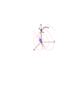
Figure 1: Schematic pattern of the electric field produced in the point ${\rm\bf r}_{0}$ by the dipole ${\rm\bf d}_{e}$ located at the coordinate origin.

Next, we calculate the potential

$$\Phi=\frac{{\bf d}_{e}\!\!\cdot\!{\bf r}_{0}}{r_{0}^{3}}\,$$ (3)

of the electric dipole ${\bf d}_{e}$ at the origin of coordinates in Fig. 1 produced in the point ${\bf r}_{0}$, where the second atom (experiencing the Stark splitting) is located. The corresponding electric field and its gradient are given by

$${\cal E}_{z}=\frac{d_{e}}{r_{0}^{3}}\,(1+3\cos^{2}\theta)^{1/2}$$ (4a)

and

$$\frac{d{\cal E}_{z}}{dz}=-\frac{3d_{e}}{r_{0}^{4}}\>\frac{3+5\cos^{2}\theta}{1+3\cos^{2}\theta}\,\cos\theta\,,$$ (4b)

respectively.

We shall consider below in detail the case of two simultaneously-excited dipoles aligned along ${\bf r}_{0}$, either in the same direction or oppositely to each other. From a physical point of view, the simultaneous excitation corresponds to processes on a time scale much smaller than the Rabi period, e.g., as in experiment Schauß et al. (2012). Then,

$${\cal E}_{z}=\frac{2d_{e}}{r_{0}^{3}},\qquad\frac{d{\cal E}_{z}}{dz}=-{\epsilon}_{\theta}\frac{6d_{e}}{r_{0}^{4}},$$ (5)

where

$${\epsilon}_{\theta}=\begin{cases}\hphantom{-}1,\quad\mbox{at }\theta=0,\\ -1,\quad\mbox{at }\theta={\pi}.\end{cases}$$ (6)

Since the electric field is treated here in the classical approximation, its source is the expectation value of the electric dipole operator $\hat{\rm\bf d}_{e}=-\hat{\rm\bf r}_{e}$, where ${\rm\bf r}_{e}$ is the radius vector of an electron inside the atom,

$$d_{e}=-\langle\,\hat{\xi}_{e}\,\rangle=-\frac{3}{2}\,n\Delta\,.$$ (7)

This matrix element is well known from the calculation of the first-order Stark effect Bethe and Salpeter (1957); Gallagher (1994); Landau and Lifshitz (1977). It is easy to see that

$${\epsilon}_{\theta}=-{\rm sign}({\Delta}).$$ (8)

In the context of Rydberg blockade, it is convenient to measure the perturbative energy shift with respect to the energy of the unperturbed original manifold $\bar{n}$ whose blockade is studied and which is denoted by a bar,

$$\delta E_{\bar{n}}=\frac{1}{2{\bar{n}}^{2}}-\frac{1}{2n^{2}}+\delta E_{n}\,.$$ (9)

Furthermore, we scale all lengths and energies with the characteristic size and energy of the state $\bar{n}$. The scaled quantities will be denoted with a tilde,

$$r_{0}={\bar{n}}^{2}\tilde{r},\quad E=\tilde{E}/(2{\bar{n}}^{2}).$$ (10)

(For conciseness, the scaled radius vector of the atom is written without subscript ‘0’.)

At last, combining (1), (5), (7)–(10), we arrive at the electronic energy-level shifts in the second atom produced by the first atom:

$$\delta\tilde{E}_{\bar{n}}^{(2)} \!\!=\!\! 1-\frac{\bar{n}^{2}}{n^{(2)2}}+9\bigg{[}\frac{1}{{\tilde{r}}^{3}}\,\frac{n^{(1)}\,n^{(2)}\,|{\Delta}^{(1)}|\,{\Delta}^{(2)}}{\bar{n}^{4}}$$ (11)

$$-\,\frac{2}{{\tilde{r}}^{6}}\,\frac{g_{2}^{(2)}n^{(1)2}{\Delta}^{(1)2}}{\bar{n}^{10}}+\frac{2}{{\tilde{r}}^{4}}\,\frac{g_{3}^{(2)}n^{(1)}{\Delta}^{(1)}}{\bar{n}^{6}}\bigg{]}.$$

The number of the particular atom is designated by a superscript in parentheses (to avoid its confusion with exponents). The energy shifts in the first atom are given, evidently, by the same expression with interchanged superscripts.

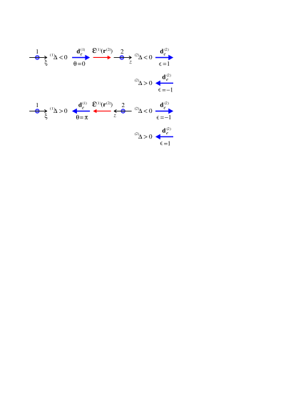
Figure 2: Sketch of possible orientations of two dipoles.

Finally, let us consider in detail two particular types of excitations in our diatomic system:

(a) $${|n_{1},n_{2},m\rangle}^{\!(1)}\,{|n_{1},n_{2},m\rangle}^{\!(2)},\;\textit{i.e.},$$

$$n\equiv n^{(1)}=n^{(2)},\quad\Delta\equiv{\Delta}^{(1)}={\Delta}^{(2)},$$

$$g_{2}^{(1)}\!=g_{2}^{(2)},\quad g_{3}^{(1)}\!=g_{3}^{(2)};$$

(b) $${|n_{1},n_{2},m\rangle}^{\!(1)}\,{|n_{2},n_{1},m\rangle}^{\!(2)},\;\textit{i.e.},$$

$$n\equiv n^{(1)}=n^{(2)},\quad\Delta\equiv{\Delta}^{(1)}=-{\Delta}^{(2)},$$

$$g_{2}^{(1)}\!=g_{2}^{(2)},\quad g_{3}^{(1)}\!=g_{3}^{(2)}.$$

In other words, both atoms are excited exactly to the same states in case (a) and to the states with interchanged parabolic quantum numbers in case (b). As is seen in Fig. 2, case (a) corresponds to the same orientation of the dipoles (directed to the right or to the left), while case (b) features oppositely oriented dipoles (either towards or away from each other). We can expect that these two cases represent two limiting situations, so that the patterns of Rydberg blockade for other orientations will lie between them.

So, the energy shifts in both atoms under the above-mentioned conditions will be the same and equal to

$$\delta\tilde{E}_{\bar{n}}\! \!\equiv\,\delta\tilde{E}_{\bar{n}}^{(1)}\!=\,\delta\tilde{E}_{\bar{n}}^{(2)}\!=1-\frac{\bar{n}^{2}}{n^{2}}+9\bigg{[}\frac{1}{{\tilde{r}}^{3}}\,\frac{n^{2}{\Delta}^{2}}{\bar{n}^{4}}\,\epsilon\>{\rm sign}(\Delta)$$ (12)

$$-\,\frac{2}{{\tilde{r}}^{6}}\,\frac{g_{2}n^{2}{\Delta}^{2}}{\bar{n}^{10}}+\frac{2}{{\tilde{r}}^{4}}\,\frac{g_{3}n\Delta}{\bar{n}^{6}}\bigg{]},$$

where

$${\epsilon}=\begin{cases}\hphantom{-}1,\;\mbox{for parallel dipoles},\\ -1,\;\mbox{for anti-parallel dipoles}.\end{cases}$$ (13)

Note that the first and second terms in square brackets in Eq. (12) result from the first- and second-order Stark effect in the uniform field, respectively; while the third term comes from the first-order perturbation by the electric field gradient.

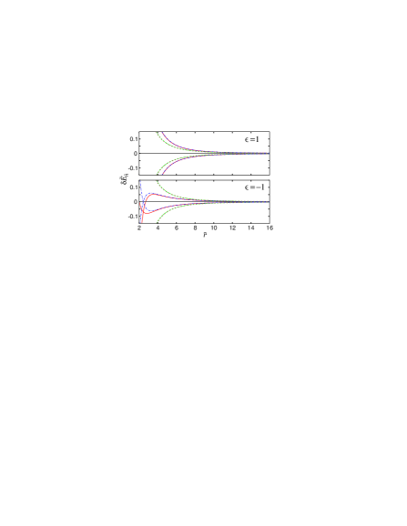
Figure 3: Energy level shifts $\delta\tilde{E}_{\bar{n}}$ for $n=\!\bar{n}\!=43$; $m=0$; $n_{1}\!=\!0$ and 42 (the most disturbed sublevels) taking into account only the first-order uniform-field Stark effect (dashed green curves), the first- and second-order uniform-field effects (dotted brown curves), the first-order uniform-field and gradient-term effects (dot-and-dashed blue curves), and all three contributions in (12) (red solid curves).

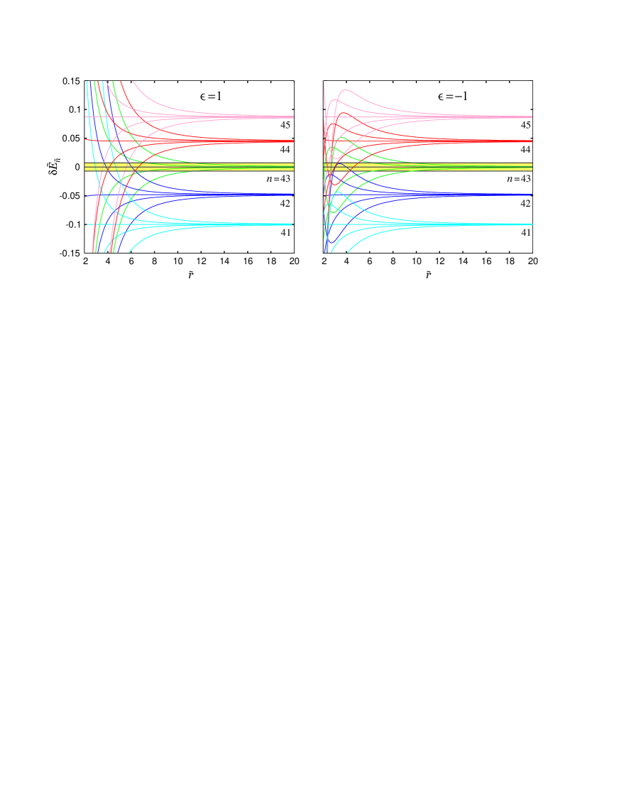
Figure 4: Stark splitting $\delta\tilde{E}_{\bar{n}}$ of energy levels as function of the interatomic distance $\tilde{r}$ for $n=\!\bar{n}\!=43,\>n_{1}\!=\!0,10,21,32,42$ (green curves), $n\!=\!42,\>n_{1}\!=\!0,10,20,31,41$ (blue), $n\!=\!41,\>n_{1}\!=\!0,10,20,30,40$ (cyan), $n\!=\!44,\>n_{1}\!=\!0,11,22,32,43$ (red), and $n\!=\!45,\>n_{1}\!=\!0,11,22,33,44$ (magenta). The horizontal shaded (yellow) strip denotes the energy excitation band of laser irradiation, $\Delta\tilde{E}=1.44{\cdot}10^{-2}$.

To reveal effects of the different perturbative terms, we have drawn in Fig. 3 a series of curves taking into account the combinations of them. For parallel dipoles ($\epsilon=1$) the following conclusions can be drawn:

• The dotted (brown) curves are almost indistinguishable from the dashed (green) curves, implying that the second-order Stark shift is negligible compared to the first-order Stark shift in the uniform field.

• There is an appreciable yet not qualitative difference between the dashed (green) and dot-dashed (blue) curves. Consequently, the gradient-term Stark effect is noticeable.

• Since the solid (red) curves almost coincide with the dot-dashed (blue) curves, the second-order Stark effect is again negligible.

With regard to anti-parallel dipoles ($\epsilon=-1$) the situation is as follows:

• Again, the dotted (brown) curves are indistinguishable from the dashed (green) curves. Hence, the second-order Stark shift can be ignored if the gradient term is not taken into consideration.

• The difference between the dashed (green) curves and the dot-dashed (blue) curves is larger than in the case $\epsilon=1$ and becomes even qualitative (the corresponding curves are bent in the opposite direction at small distances). Therefore, the gradient-term Stark effect plays an important role.

• One also sees that the solid (red) curves are shifted downwards with respect to the dot-dashed (blue) curves at small $\tilde{r}$. Hence, in principle, the second-order Stark effect becomes noticeable but does not play a crucial role.

In summary, we can say that the gradient term is always important and can even qualitatively change the behavior of energy curves at small $\tilde{r}$ in the case of anti-parallel dipoles. On the other hand, one can usually neglect the second-order Stark effect in the uniform field. It becomes noticeable only at small distances in the case of anti-parallel dipoles, when the first-order perturbations by the uniform field and the gradient term compensate each other to a large extent.

Returning to the problem of breaking the Rydberg blockade, we show in Fig. 4 examples of a few Stark-split energy levels for the parameters of experiment Schauß et al. (2012), where ${}^{87}{\rm Rb}$ with $\bar{n}=43$ and $m=0$ was used. For better visibility, the energy excitation band $\Delta\tilde{E}$ (yellow stripe) was taken here 100 times larger than in the experiment. Besides, to avoid excessive complication of the figure, we have not shown the avoided crossings, because they do not affect the total density of energy levels in the excitation band.

The pattern of levels for $\epsilon=1$ is approximately symmetric with respect to their asymptotic degenerate positions, in qualitative agreement with our earlier considerations Dumin (2014). On the other hand, for anti-parallel dipoles ($\epsilon=-1$) the levels show nonmonotonic and asymmetric behavior.

At sufficiently large distances, all levels of the $n=43$ manifold are within the excitation band. When $\tilde{r}$ decreases, these levels begin to deviate from the horizontal line and leave the excitation band such that the Rydberg blockade develops. However, when the distance decreases further, down to $\tilde{r}=5-6$, the strongly-perturbed energy levels from the neighboring Stark manifolds (or even the levels from the same manifold $n=43$ bent in the opposite direction) enter the excitation band, thereby lifting the Rydberg blockade. As can be seen in this figure, at $\epsilon=1$ the blockade is lifted by both the upper- and lower-lying Stark manifolds. In contrast, for $\epsilon=-1$ the contribution comes mostly from the upper-lying manifolds.

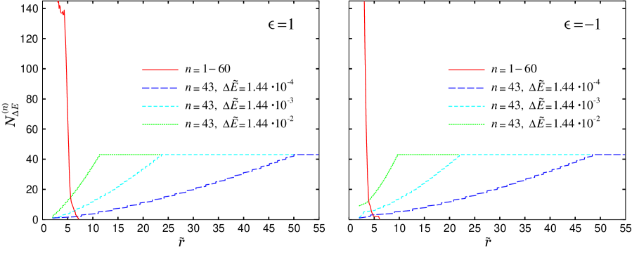
Figure 5: The number of energy levels $N_{\Delta E}^{(n)}$ within the running window $\Delta\tilde{r}=1$ for various bandwidths $\Delta\tilde{E}$ of the exciting irradiation and different Stark manifolds $n$.

The total effect of the level shifts is illustrated in Fig. 5, which represents the total number of energy levels $N_{\Delta E}^{(n)}$ in the excitation band $\Delta\tilde{E}$ within a running window $\Delta\tilde{r}=1$ (i.e., the characteristic size of the Rydberg atom). The dashed and dotted (blue, cyan, and green) curves show the number of levels of the basic manifold $n=43$ remaining within the excitation band as function of the distance. Not unexpected, the narrower the excitation band, the larger is the Rydberg blockade zone. The experimental bandwidth in Schauß et al. (2012) was very small, $\Delta\tilde{E}=1.44{\cdot}10^{-4}$, corresponding to the long-dashed (blue) curves in Fig. 5 that drop off at the largest distance ($\tilde{r}{\leqslant}50$) and vary most gradually.

The red curve, sharply rising at small distances indicates lifting of the Rydberg blockade by the Stark-split energy levels from the neighbouring manifolds. It is approximately independent of $\Delta\tilde{E}$, since the strongly-perturbed energy levels enter the excitation band almost vertically. The upper limit of $n$, until which the energy levels are counted, is somewhat arbitrary but certainly limited by the range of validity of the perturbative Stark splitting. The latter is roughly given by the condition that the energy shift should be less than the absolute value of the unperturbed energy: $|E_{\bar{n}}|-|E_{n}|\lesssim|E_{n}|$, implying $n\lesssim\sqrt{2}\,\bar{n}$. Hence, for $\bar{n}=43$, we get an upper limit of $n\approx 60$. On the other hand, it can be easily seen that perturbation theory is applicable to all the low-lying levels, because the criterion $|E_{n}|-|E_{\bar{n}}|\lesssim\,|E_{n}|$ is always satisfied for $n<\bar{n}$.

Note that despite the qualitatively different patterns of individual energy levels for $\epsilon=1$ and $-1$ (Fig. 4), the resulting effect on the Rydberg blockade is almost the same: the left and right panels of Fig. 5 are very similar to each other; only the blockade-lifting red peak is narrower for the anti-parallel dipoles.

The values for the outer boundary of the Rydberg blockade zone ($\tilde{r}=50$ at $\Delta\tilde{E}=1.44{\cdot}10^{-4}$) and the inner boundary, where the blockade breaks down ($\tilde{r}=5$), correspond very well to the measurements presented in Fig. 3a of Schauß et al. (2012). For the comparison of the experimental and theoretical plots, one should keep in mind that 1 $\mu$m corresponds to 9.8 dimensionless units of length used in the present paper. In passing, we note that the additional excitation zones, formed by the neighboring Stark manifolds, merge into one broad shell about $\tilde{r}=0$. Therefore, the individual thin shells (qualitatively discussed in Dumin (2014)) can be hardly resolved under realistic experimental conditions.

III Discussion

Strictly speaking, our study refers only to hydrogen-like atoms without quantum defects. They were taken into account recently in Derevianko et al. (2015), whose authors employed the idea of quasi-molecular levels of two nearby Rydberg atoms. Calculating in detail such levels for the 100s state of rubidium, they obtained the probabilities of detrimental excitation (or the “molecular loss rates”) for a few unblocked shells. It was found that the most significant effect, i.e., the largest excitation rate, is produced by the outermost unblocked shell. Since it is affected least by the quantum defects, neglecting them should be reasonable in many situations.

Relevant is also the size of the outermost shell $R_{\rm b}$, which we estimate in the following to exponential accuracy (i.e., ignoring pre-exponential factors on the order of unity). In the framework of the quasi-molecular (qm) model one gets

$$R_{\rm b}^{\rm(qm)}\!\propto n^{8/3}\approx n^{2.67},$$ (14a)

see Sec. II in Ref. Derevianko et al. (2015). On the other hand, our earlier treatment of the Rydberg blockade in terms of the Stark effect in the uniform field (uS) gives

$$R_{\rm b}^{\rm(uS)}\!\propto n^{7/3}\approx n^{2.33},$$ (14b)

see formula (14) in Ref. Dumin (2014). At last, the same treatment for the strongly nonuniform field (nS) results in formula (36) of Ref. Dumin (2015) with

$$R_{\rm b}^{\rm(nS)}\!\propto n^{9/4}\approx n^{2.25}.$$ (14c)

Hence, all three approximations give similar results with the quasi-molecular model predicting the steepest dependence on the principal quantum number.

Clearly, the quasi-molecular treatment appears to be more accurate, because it takes into account the structure of energy levels of a particular atom at the expense of a cumbersome computation and the loss of general relevance. Our approach based on Stark splitting is of complementary value, offering a simple and straightforward determination of the blockade breaking from a general perspective, omitting possible additional features, different for each atom. It can be especially valuable for reasonable estimates in situations where it is unknown in advance which chemical element and which of its states could be employed best for the quantum information processing.

Besides and most importantly, our approach explains transparently why the pair correlation function of Rydberg atoms is never equal to zero in the blockaded volume (e.g., Fig. 3a of Ref. Schauß et al. (2012)), whereas this fact is not so clear from the quasi-molecular model Derevianko et al. (2015).

Yet another method of treating the interactions between Rydberg atoms is the multipole expansion Flannery et al. (2005). It is based on the same physical assumptions as our calculation of the gradient-term Stark effect Dumin (2015), namely, the first-order perturbation theory with respect to the product state of two unperturbed atoms. However, the multipole expansion results in a lot of cumbersome terms, making a subsequent analysis necessary which of them are really important in the respective context. In contrast, the treatment based on the gradient term “automatically” takes into account the most important contributions just from the beginning. Hence, it has the same physical accuracy as the multipole techniques but works more efficiently for our needs.

Finally, let us mention that also non-additive perturbations in the systems containing more than two atoms can break the Rydberg blockade. Such a situation for three atoms was considered in paper Pohl and Berman (2009).

IV Conclusions

In summary, we have developed an analytical model, sufficiently general to be used in order to refine certain properties of the Rydberg blockade. Firstly, we conclude that lifting the Rydberg blockade at small interparticle distances has a universal physical reason, rather than being a result of experimental imperfections. This effect should be kept in mind in the design of future high-precision experiments, e.g., for quantum information processing.

Secondly, our description in terms of the Stark-split manifolds naturally explains also why the probability of excitation remains nonzero in the major part of the blockaded volume. This is yet another inherent property of the Rydberg blockade, rather than the effect of “imperfect removal of the ground-state atoms” in Schauß et al. (2012).

Finally, the treatment of the Rydberg blockade performed in the present paper refers to the coherent (simultaneous) excitation of Rydberg atoms. If the excitation of atoms is incoherent (sequential), as assumed in our previous works Dumin (2014, 2015), the Rydberg blockade should also be lifted at small distances but can possess some specific features, which still have to be studied in detail. This may be interesting, e.g., for the experiments with ultracold plasmas performed on much longer time scales Robert-de Saint-Vincent et al. (2013).