Statistical Test of Distance–Duality Relation with Type Ia Supernovae and Baryon Acoustic Oscillations

Abstract

We test the distance–duality relation $\eta\equiv d_{\text{L}}/[(1+z)^{2}d_{\text{A}}]=1$ between cosmological luminosity distance ($d_{\text{L}}$) from the JLA SNe Ia compilation and angular-diameter distance ($d_{\text{A}}$) based on Baryon Oscillation Spectroscopic Survey (BOSS) and WiggleZ baryon acoustic oscillation measurements. The $d_{\text{L}}$ measurements are matched to $d_{\text{A}}$ redshift by a statistically consistent compression procedure. With Monte Carlo methods, nontrivial and correlated distributions of $\eta$ can be explored in a straightforward manner without resorting to a particular evolution template $\eta(z)$. Assuming independent constraints on cosmological parameters that are necessary to obtain $d_{\text{L}}$ and $d_{\text{A}}$ values, we find 9% constraints consistent with $\eta=1$ from the analysis of SNIa + BOSS and an 18% bound results from SNIa + WiggleZ. These results are contrary to previous claims that $\eta<1$ has been found close to or above the $1\sigma$ level. We discuss the effect of different cosmological parameter inputs and the use of the apparent deviation from distance–duality as a proxy of systematic effects on cosmic distance measurements. The results suggest possible systematic overestimation of SNIa luminosity distances compared with $d_{\text{A}}$ data when a Planck CDM cosmological parameter inference is used to enhance the precision. If interpreted as an extinction correction due to a gray dust component, the effect is broadly consistent with independent observational constraints.

2018 July 12

1 Introduction

A generic property of cosmological distances in general relativity is that the angular-diameter distance $d_{\text{A}}$ and the luminosity distance $d_{\text{L}}$ to the same cosmological redshift $z$ satisfy the distance–duality (DD) relation (Ellis, 1971, 2009)

$$\eta\equiv\frac{d_{\text{L}}(z)}{(1+z)^{2}d_{\text{A}}(z)}=1.$$ (1)

The theoretical underpinnings of this relation are the geometrical reciprocity relation (Etherington, 1933, 2007) that holds in any metric theory of gravity and the fact that light propagates along null geodesics with the photon number conserved. This is not the case in nonmetric theories of gravity, theories of varying fundamental constants, or axion–photon mixing models (Bassett & Kunz, 2004; Uzan et al., 2004). Therefore, an observational falsification of Equation (1) could be a useful probe of exotic physics, provided that cosmic distance measurements are exempt from astrophysical systematic effects (e.g., see Corasaniti, 2006, for violations induced by intergalactic dust extinction).

Several cosmological probes can be used for this purpose. Luminosity distances are indicated by the brightness of Type Ia supernovae (SNIa) through the standard-candle relation, and angular-diameter distances can be inferred from the apparent size of cosmic standard rulers. Numerous studies devoted to testing the validity of Equation (1) have used SNIa $d_{\text{L}}$ data in combination with $d_{\text{A}}$ estimates from X-ray observations of galaxy clusters (e.g., Bassett & Kunz, 2004; Uzan et al., 2004; De Bernardis et al., 2006; Holanda et al., 2010; Santos-da-Costa et al., 2015). However, angular distance measurements from galaxy cluster observations are cosmological-model dependent (see, e.g., Bonamente et al., 2006). Furthermore, astrophysical uncertainties such as the three-dimensional profile of intra-cluster plasma may significantly affect the estimation of $d_{\text{A}}$ (Meng et al., 2012; Yang et al., 2013). Recent works have instead used angular-diameter distance measurements from observations of strong lens systems (Holanda et al., 2016, 2017; Liao et al., 2016; Fu & Li, 2017; Rana et al., 2017). These estimates have the advantage of being cosmological-model independent, but they are not exempt from systematic effects. In fact, lens mass model uncertainties due to the mass-sheet degeneracy and the effect of external perturbators may have a strong impact on the inferred properties of these systems (Schneider & Sluse, 2013). More reliable estimates can be derived from the baryon acoustic oscillation (BAO) signal in the galaxy power spectrum. Although they depend on the cosmic matter density and the Hubble constant, thus demanding prior external information, these only contribute to statistical uncertainties. In contrast, systematic effects due to the nonlinearity of the matter density field are largely sub-dominant, as they are expected to alter $d_{\text{A}}$ estimates to less than a few percent level (Crocce & Scoccimarro, 2008; Rasera et al., 2014).

A common approach to test the DD relation uses distance measurements to constrain parameterizations of $\eta$ as a function of redshift $z$ (e.g. Nair et al., 2012; Wu et al., 2015; Holanda et al., 2016, 2017; Liao et al., 2016; Fu & Li, 2017). The choice of an $\eta(z)$ template function imposes a strong prior on the DD analysis, which may result in different outcomes depending on its form. In our view, a template-free study is preferred because of its generality and robustness in the absence of abundant data.

A practical issue underlying the tests is the fact that measurements of $d_{\text{L}}$ and $d_{\text{A}}$ may not be available at the same redshift. Several studies have attempted to address this problem by selecting data points under a proximity criterion, e.g., by only using data within a redshift separation $\left|\Delta z\right|\leq 5\times 10^{-3}$ (Holanda et al., 2010). However, this may incur the penalty of significantly reduced statistical information encoded in the data sets. Moreover, it does not guarantee that the data points thus chosen provide a representative local sample. This situation is analogous to the problem of estimating the cross-correlation of unevenly sampled time-series data, for which narrow windows centered on cherry-picked data can lead to a spuriously high significance of detection (Max-Moerbeck et al., 2014).

To overcome the redshift-matching problem, Cardone et al. (2012) have applied a local regression technique to the SNIa $d_{\text{L}}$ data at redshift windows of interest with adjustable bandwidth. However, this method is not easily generalized to highly correlated data. It still rejects the majority of data points outside of the narrow windows, and one might overlook their influence on $d_{\text{L}}$ estimates through their systematic correlations with data points inside the windows.

Here, we address the issue by using a Bayesian statistical method detailed in Ma et al. (2016, hereafter M16), which compresses correlated luminosity distance data at given control points in log-redshift. This has been specifically developed for the analysis of the SNIa data from the Joint Light-curve Analysis (JLA; Betoule et al., 2014). The goal of this work is to provide up-to-date, straightforward, and independent measurements of $\eta$ at selected redshifts, along with their correlations, using $d_{\text{L}}$ from the compressed JLA data set and $d_{\text{A}}$ estimates from BAO measurements. The derived constraints are largely limited by the uncertainties on the cosmological parameters that the $d_{\text{A}}$ values depend on. Combining external information from Planck measurements of the cosmic microwave background (CMB) temperature and polarization anisotropy power spectrum (Planck Collaboration, 2016a) can significantly reduce such uncertainties. However, as we will amply explain, Planck-derived constraints on cosmological parameters implicitly assume that there is no violation of the photon number conservation. In such a case, the DD test can be used as probe of systematic effects affecting the luminosity distance or the angular-diameter distance measurements.

In Section 2, we derive expressions for $d_{\text{L}}$ and $d_{\text{A}}$ in terms of the data. In Section 3, we describe the Monte Carlo (MC) analysis methods. The results are presented and analyzed in Section 4 and further discussed in Section 5.

2 Data Sets

2.1 BAO Angular-diameter Distance

We use $d_{\text{A}}$ estimates from BAO measurements of the WiggleZ survey (Blake et al., 2011a, 2012) and the Baryon Oscillation Spectroscopic Survey (BOSS) DR12 (Alam et al., 2017) consensus compilation. WiggleZ data consist of BAO volume distance parameter $A(z)$ (Eisenstein et al., 2005; Blake et al., 2011a) and the Alcock–Paczyński effect parameter $F(z)$ (Ballinger et al., 1996; Blake et al., 2011b) at effective redshifts 0.44, 0.60, and 0.73, respectively. From the measurements, $d_{\text{A}}$ is derived through the following equation

$$d_{\text{A,WiggleZ}}(z)=\frac{c}{H_{0}}\frac{A(z)[z^{2}F(z)]^{1/3}}{\sqrt{\Omega_{\text{m}}}(1+z)},$$ (2)

where $c$ is the speed of light, $H_{0}$ is the Hubble constant, and $\Omega_{\text{m}}$ is the matter density parameter.

BOSS data on the other hand provide consensual estimates of the ratio $\widetilde{d}_{M}=d_{\text{A}}(1+z)r_{\text{d}}^{\text{fid}}/r_{\text{d}}$ by joining the constraints from BAO features and the full shape of galaxy correlations at effective redshifts 0.38, 0.51, and 0.61. Here, $r_{\text{d}}$ is the acoustic horizon at the photon–baryon drag epoch and the BOSS DR12 fiducial value is $r_{\text{d}}^{\text{fid}}=147.78$ Mpc. Thus, $d_{\text{A}}$ is expressed in terms of the data by

$$d_{\text{A,BOSS}}(z)=\frac{r_{\text{d}}}{r_{\text{d}}^{\text{fid}}}\frac{\widetilde{d}_{M}(z)}{(1+z)}.$$ (3)

We notice that the overlap of WiggleZ and BOSS survey volumes makes the two BAO data sets correlated (Beutler et al., 2016). However, a full analysis consistently joining the data sets is beyond the scope of this work.

Evidently from Equations (2) and (3), in order to use the BAO data, it is necessary to specify the cosmological parameters, or “complementary parameters” (CPs), namely $\boldsymbol{\varphi}=(H_{0},\Omega_{\text{m}},r_{\text{d}})$. The CPs are similar to the role of prior distributions in the context of inference problems, in that they are specified independently of and in complement to the data to express our belief or uncertainty. However, unlike prior distributions, they cannot be updated by the analysis. In Section 3 we describe the choice of such CPs in detail.

2.2 SNIa Luminosity Distance

We compute compressed SNIa luminosity distance moduli $\mu_{\text{Lc}}$ and their covariance matrix from the JLA data set with the method detailed in M16. The redshifts of compression, or “control points,” are chosen with two criteria in mind. First, $\mu_{\text{Lc}}$ must be available at the redshift of $d_{\text{A}}$ data. Second, the control points should be distributed such that the statistical uncertainties on $\mu_{\text{Lc}}$ are evenly imputed to them. In practice, we perform two separate compression runs for SNIa + BOSS and SNIa + WiggleZ respectively. Each compressed data set contains 15 suitably chosen control points between $0.01\leq z\leq 1.30$, and the relevant data portions are listed in Table 1. We have verified that the compression results are not affected significantly by the choice of other control points.

Table 1: Compressed SNIa Data at Anchoring and BAO-matching Control Points

$z$	$\mu_{\text{Lc}}$	$\text{Covariance}\times 10^{4}$
SNIa + BOSS
0.01	33.12 ±0.05	21.18	2.392	1.625	1.395
0.38	41.57 ±0.03	$\cdots$	8.925	0.192	2.450
0.51	42.30 ±0.03	$\cdots$	$\cdots$	10.05	1.869
0.61	42.74 ±0.03	$\cdots$	$\cdots$	$\cdots$	12.02
SNIa + WiggleZ
0.01	33.12 ±0.05	21.69	2.115	1.341	0.067
0.44	41.93 ±0.03	$\cdots$	8.636	1.023	3.238
0.60	42.70 ±0.03	$\cdots$	$\cdots$	9.746	4.636
0.73	43.21 ±0.05	$\cdots$	$\cdots$	$\cdots$	26.00

Note. — Covariance values have been scaled by $10^{4}$ for presentation.

It should be noted that the compression step computes the distance moduli only up to an implicit magnitude offset $M$. It is the quantity

$$\mu_{\text{Lc}}=\mu_{\text{L}}-M=5\log_{10}\left(\frac{d_{\text{L}}}{10\leavevmode\nobreak\ \text{pc}}\right)-M$$ (4)

that is produced by the compression. The parameter $M$ in Equation (4) is degenerate with $H_{0}$ as discussed in M16 (see also Yang et al., 2013), and it is possible to eliminate $M$ and to obtain $d_{\text{L}}$ that is directly comparable to $d_{\text{A}}$. We exploit the fact that at the lowest available, or the “anchoring” redshift $z_{1}=0.01$, the luminosity distance can be approximated to the second order as

$$d_{\text{L}}(z_{1})=\frac{cz_{1}}{H_{0}}\left[1+\frac{1}{2}\left(1-q_{0}\right)z_{1}+\mathcal{O}(z_{1}^{2})\right]\approx\frac{cz_{1}}{H_{0}},$$ (5)

where $q_{0}$ is the deceleration parameter. For the small value of $z_{1}$, higher-order terms in Equation (5) are negligible (unless one must consider unrealistic cosmological scenarios with $\left|q_{0}\right|\approx 10^{2}$). This allows us to express $M$ by $d_{\text{L}}(z_{1})\approx cz_{1}/H_{0}$ and $\mu_{\text{Lc}}(z_{1})$ using Equation (4). Carrying out the algebra, we obtain the expression for $d_{\text{L}}(z)$ as

$$d_{\text{L}}(z)=\left(\frac{cz_{1}}{H_{0}}\right)10^{\left[\mu_{\text{Lc}}(z)-\mu_{\text{Lc}}(z_{1})\right]/5}.$$ (6)

3 Methods

We derive the probability density function (PDF) of $\eta$ at a given redshift from MC samples of $d_{\text{L}}$ and $d_{\text{A}}$ inferred from the observational data sets. The underlying idea is that the SNIa and BAO distance data, the CPs, and $\eta$ at the chosen redshifts are all random variables. In particular, $\eta$ is a transformation of the combined random variable of data and CPs, which is specified by the composition of Equation (1) with Equation (6) and either Equation (2) or (3) for WiggleZ or BOSS data, respectively.

The view of observational data as random variables fits naturally into the Bayesian statistical inference framework commonly encountered in the study of cosmological models (for example, see M16, Section 2). The CPs themselves are often obtained from Bayesian inference with observational data. In such a case, a self-consistent analysis demands that the inference of CPs does not rely on the $d_{\text{A}}$ and $d_{\text{L}}$ data sets used here, and that the underlying statistical model used in the CP inference does not put restrictive assumptions on $\eta$ or related functions.

In practice, it can be difficult to unambiguously satisfy both these points, and we must also be attentive to the context of their validity. Still, we can make our best efforts in this direction.

3.1 Complementary Parameters

Following the discussion in Section 2.1, in order to estimate the BAO angular-diameter distances, we need input on the CPs, $\boldsymbol{\varphi}=(H_{0},\Omega_{\text{m}},r_{\text{d}})$, while for SNIa data we need to incorporate the dependence on $H_{0}$. In this work, we consider two CP sets motivated by current knowledge of those parameters from independent observations.

The first CP set consists of a joint distribution on $(h,\Omega_{\text{m}},\Omega_{\text{b}}h^{2})$ where $h=H_{0}/100\leavevmode\nobreak\ \text{km\leavevmode\nobreak\ s}^{-1}\leavevmode\nobreak\ \text{Mpc}^{-1}$ is the dimensionless Hubble constant and $\Omega_{\text{b}}h^{2}$ the baryon energy density parameter. We sample $h$ from a conservative choice, namely the Gaussian distribution $\mathcal{N}(0.688,0.033^{2})$ used in M16 based on the re-selected and re-calibrated nearby SNIa distances with the independent megamaser distance to NGC 4258 as the Cepheid zero point (Rigault et al., 2015). The usefulness of NGC 4258 as a calibration source with independent, well-understood systematic uncertainties is explained by Efstathiou (2014). We further adopt the conservative estimate $\Omega_{\text{b}}h^{2}\sim\mathcal{N}(0.02228,0.00084^{2})$ from a big-bang nucleosynthesis analysis with relic [4][]He and deuterium abundance data (Cyburt et al., 2016, table V). For $\Omega_{\text{m}}$, we use a simple, non-informative distribution, namely the uniform distribution over the range [0.15, 0.45], which is inclusive enough to cover independent constraints from the mass function of galaxy clusters (Bocquet et al., 2015). Furthermore, as an indirect check on these choices, we compute the baryon fraction $f_{\text{b}}=\Omega_{\text{b}}/\Omega_{\text{m}}$ as implied by the random samples. The resultant $f_{\text{b}}$ distribution, with mean and standard deviation 0.17 $\pm$ 0.06, is consistent with independent constraints from galaxy cluster observations (Gonzalez et al., 2013; Chiu et al., 2016).

In order to check the sensitivity of the results to the particular choice of $h$, we also derive constraints by sampling $h$ from a Gaussian distribution with $\mathcal{N}(0.7348,0.0166^{2})$ based on the Cepheid period–luminosity relation determined by parallaxes of Milky Way Cepheids (Riess et al., 2018). The other parameters’ distributions are unmodified. We will refer to this alternative CP set as “H73.”

From these random samples, we derive the sample for $r_{\text{d}}$, which is necessary for application with BOSS BAO distances. Following the discussions in Mehta et al. (2012) and Anderson et al. (2014), we evaluate $r_{\text{d}}$ as a function of $(h,\Omega_{\text{m}},\Omega_{\text{b}}h^{2})$ using the software CAMB (Lewis et al., 2000, 2017) with the other cosmological parameters fixed at the values of the BOSS fiducial CDM model specified in Alam et al. (2017). The CP set thus generated is denoted by the label “Synthetic” in the rest of this paper, for it is based on the combination of independent observation constraints. The sample size is $2\times 10^{6}$.

The other CP choice is based on the Markov chain MC analysis for the Bayesian cosmological parameter constraints of the KiDS-450 tomographic weak lensing (WL) survey (Hildebrandt et al., 2017), including posterior samples for $H_{0}$, $\Omega_{\text{m}}$, and $r_{\text{d}}$. They are valuable as an independent, data-informed source for $\Omega_{\text{m}}$ and $r_{\text{d}}$. However, WL alone offers no informative update on its $H_{0}$ prior. If one had accepted the $H_{0}$ constraint as it is, value ranges far removed from informative observational measurements (such as Riess et al., 2016, 2018; Abbott et al., 2017) would have been over-weighted. For this reason, we perform a re-weighting of the Markov chains by a weighting function $f_{h}$, the Gaussian PDF underlying the $h$ distribution in the Synthetic CP set. The re-weighting is implemented with an accept–reject MC algorithm. For each sample point in the KiDS-450 Markov chain output, it is randomly accepted with the suitably normalized probability $p\propto f_{h}$. Overall, the acceptance rate is about 32.6%, leaving a sample size of about $6.9\times 10^{5}$. We have verified that the induced shifts in the distributions of $\Omega_{\text{m}}$ and $r_{\text{d}}$ are about $0.1\sigma$. This confirms that the $h$-based re-weighting does not contaminate the relevant WL-inferred cosmological parameters noticeably. We thus obtain an alternative CP set, and for simplicity, in the following sections we refer to it as “KiDS.”

3.2 Cosmic Distance Samples

We now discuss the random samples of $d_{\text{L}}$ and $d_{\text{A}}$ generated from the observational data sets described in Section 2. Their distributions are well-approximated by multivariate Gaussian random variables. We generate the two samples separately and verify that they are not correlated with the CP samples. In the case of the WiggleZ BAO data, we generate the $(A,F)$ joint Gaussian sample using the mean vector and covariance matrix of Blake et al. (2012), having marginalized over the growth rate parameter $f\sigma_{8}$. This is combined with the CP samples through Equation (2) to obtain the sample of $d_{\text{A,WiggleZ}}(z)$. In the case of BOSS data, the Gaussian sample of $\widetilde{d}_{M}$ is created using the mean and covariance values of Alam et al. (2017), having marginalized over the $r_{\text{d}}$-scaled expansion rate $(r_{\text{d}}/r_{\text{d}}^{\text{fid}})H$ and $f\sigma_{8}$. Then, by combining through Equation (3) the $\widetilde{d}_{M}$ sample with that of $r_{\text{d}}$, we obtain the sample of $d_{\text{A,BOSS}}(z)$.

For the SNIa data, we generate Gaussian samples of $\mu_{\text{Lc}}$ based on the compressed distance moduli described in Section 2.2. Combining them with $H_{0}$ through Equation (6), we obtain the $d_{\text{L}}$ samples.

Finally, by combining the $d_{\text{A}}$ and $d_{\text{L}}$ samples, we derive $\eta$ through its definition in Equation (1) as two distinct samples from SNIa + WiggleZ and SNIa + BOSS respectively. In each case, the data sample size is matched with the CP sample. It is worth noticing that the distance scale $c/H_{0}$ is eliminated by combining Equations (2) and (6). As a result, the $\eta$ distribution from SNIa + WiggleZ is independent of $H_{0}$. This is not true for SNIa + BOSS, because $r_{\text{d}}$ deviates from the scaling $r_{\text{d}}\propto H_{0}^{-1}$ due to the effect of cosmic expansion rate on early-Universe matter-to-radiation ratio (Hu et al., 1995) and recombination rates (Seager et al., 2000).

4 Results

4.1 Testing the DD Relation

We derive constraints on $\eta$ from the analysis of SNIa + BOSS and SNIa + WiggleZ samples separately. Figure 1 shows the mean and standard deviation estimated from the random samples, and the corresponding values are quoted in Table 2. In Figure 1, we also show the constraints inferred using H73. As we can see, despite the discrepancy between the choices of $h$ distribution, it has no significant effect on the inferred bounds on $\eta$. Here, we stress again that results from different BAO surveys cannot be combined trivially. In the case of the KiDS CP, because the analysis partially depends on Markov chains, we have used the method of batch means (Flegal et al., 2008) to verify that the $\eta$ samples provides sufficiently accurate sample statistics and that the values of the mean and standard deviation reported here do not exceed their significant figures.

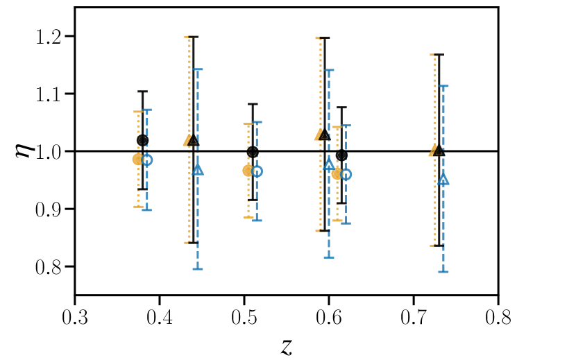
Figure 1: Marginal mean and standard deviation of $\eta$. Results with the Synthetic CP are shown in black as filled markers with solid error bars, and those with the KiDS CP are shown in blue and as open markers with dashed error bars. Results with H73 are shown in orange (dotted). SNIa + BOSS results are shown as circles, and those from SNIa + WiggleZ as triangles. For readability, the redshift locations are shifted slightly around their actual values.

Table 2: Statistical Summary of the DD Test Random Variable $\eta$

$z$	Synthetic	KiDS	Synthetic	KiDS
SNIa + BOSS
0.38	1.02 ±0.08	0.98 ±0.09	1.06^+0.06_-0.13	0.96^+0.10_-0.08
0.51	1.00 ±0.08	0.96 ±0.08	1.04^+0.06_-0.12	0.95^+0.10_-0.08
0.61	0.99 ±0.08	0.96 ±0.08	1.03^+0.06_-0.12	0.94^+0.10_-0.08
SNIa + WiggleZ
0.44	1.02 ±0.18	0.97 ±0.17	1.06^+0.14_-0.24	0.92^+0.20_-0.16
0.60	1.03 ±0.17	0.98 ±0.16	1.12^+0.10_-0.27	0.93^+0.19_-0.15
0.73	1.00 ±0.17	0.95 ±0.16	1.08^+0.10_-0.26	0.91^+0.19_-0.15

We find the $\eta$ sample distributions to be skewed. Hence, the statistical uncertainties can be characterized more precisely by a mode and credible interval analysis. To this end, we use a Gaussian kernel density estimator to overcome MC noise and smooth the sample distribution. Then, we find the approximate location of the mode for the smoothed one-dimensional marginal distribution at each redshift. The mode estimates and the $68.3\%$ credible intervals are quoted in Table 2.

The $\eta$ distributions obtained from this analysis are correlated from one redshift to another. This can be better appreciated in Figures 2 and 3, which show the two-dimensional joint constraints from SNIa + BOSS and SNIa + WiggleZ, respectively.

Figure 2: Two-dimensional MC distribution of $\eta$ from SNIa + BOSS. Each contour set encloses a region measuring $p_{1}=0.683$ (inner, thick) and $p_{2}=0.954$ (outer, thin) under the corresponding sample distribution. Solid (black) contours show the results with Synthetic CPs, and the dashed (blue) ones with the KiDS. The mean value for each case is shown by a marker of the matching color.

Figure 3: Similar to Figure 2 but from SNIa + WiggleZ and with different scales.

These results indicate the absence of substantial evidence for deviations from Equation (1). Moreover, there is no clear trend of $\eta(z)$ evolution.

From Section 3, we can readily understand that the large statistical uncertainties on $\eta$ are a consequence of the quality of both the distance data and the CPs. Tighter CPs can be used at the cost of generality, and as previously noted, when testing the DD relation, one must pay attention to the assumptions under which the CPs have been derived. In particular, one may be inclined to include one of the most stringent constraints on the cosmological parameters, namely the results from Planck measurements of CMB anisotropy power spectra (Planck Collaboration, 2016a). However, such results implicitly assume the photon number conservation and the validity of the DD relation. Any process violating the photon number conservation during the photon–baryon coupling epoch or the propagation of CMB photons will likely induce temperature anisotropy and modify the power spectra, eventually leading to a different cosmological parameter inference. Unfortunately, the effects of photon-number violating processes on CMB are highly model-specific (see, e.g., Räsänen et al., 2016). As such, tight constraints on $\eta$ obtained by including CMB information are difficult to interpret (see also Chluba, 2014).

However, this does not imply that the incorporation of CMB constraints (and implicitly their assumptions) cannot lead to a meaningful comparison between the SNIa and BAO cosmological distances. In fact, one can assume the DD relation to be valid and use the inferred constraints on $\eta$ as a proxy of potential systematics affecting cosmic distance estimations. The nature of these systematic effects does not have to be exotic physics to which CMB anisotropies are sensitive, but rather the result of unaccounted for yet mundane mechanisms independent of the CMB. As an example, in Evslin (2016) the validity of DD was used to test the calibration of the SNIa standard-candle relation. Hereafter, we will present results on cosmic distance systematics using the DD estimates in combination with a CMB-informed CP.

4.2 Cosmic Distance Systematics

In the following, we assume the DD relation to hold and use the estimates of $\eta$ from SNIa and BAO in combination with Planck results to derive constraints on systematics affecting cosmic distance measurements. In particular, we take the CPs $(H_{0},\Omega_{\text{m}},r_{\text{d}})$ (see Section 3.1), from the posterior Markov chains of the flat CDM “base” model parameters obtained from the Planck TT + TE + EE + low-$\ell$ temperature and polarization (“lowP”) anisotropy. Again, we have checked that there is minimal correlation between the chains and the data samples. We dub this CP set as “Planck.” Its sample size is about $1.07\times 10^{5}$.

In the case of SNIa $d_{\text{L}}$ measurements, systematic effects may arise from a variety of sources (see, e.g., Goobar & Leibundgut, 2011). As suggested in Corasaniti (2006), one way of using the estimates on the deviations from the DD relation is to test the presence of dust extinction due to an intergalactic gray dust component that is not removed through standard color analysis. This extinction would systematically dim SNIa, thus making them appear more remote, but would not affect the BAO distance as indicated by the shape and location of the acoustic peak in the galaxy correlation functions.

In such a case, the rest-frame B-band extinction correction to the SNIa standard-candle magnitude, $A_{B}$, is related to $\eta$ by $A_{B}(z)-A_{B}(z_{1})=5\log_{10}\eta(z)$, where, again, $z_{1}=0.01$ is the anchoring redshift (see Section 2.2). At that low redshift, the optical depth and intergalactic extinction is typically negligible. Therefore, in the remainder of this paper, we will simply refer to $A_{B}(z)$.

Table 3 displays the mean and standard deviation of the extinction $A_{B}$. These values are shown at their respective redshifts in Figure 4. Again, batch means are used to check the accuracy of these results. The $A_{B}$ samples are sufficiently symmetric when marginalized to each redshift, and the credible interval analysis reveals no substantial difference from $1\sigma$ bounds. As a joint distribution, the SNIa + BOSS result is closely approximated by the multivariate Gaussian. For future reference, we report the tests for normality and the MC estimates for its mean vector and covariance matrix in Appendix A.

Table 3: Mean and Standard Deviation of the Extinction Correction $A_{B}$ Marginalized at Each Redshift Using Planck-based CP Sets.

$z$	Planck	Planck-$w$CDM
SNIa + BOSS
0.38	0.10 ±0.06	string0.01 ±0.11
0.51	0.05 ±0.06	-0.03 ±0.12
0.61	0.04 ±0.07	-0.05 ±0.12
SNIa + WiggleZ
0.44	0.11 ±0.20	string0.03 ±0.22
0.60	0.14 ±0.14	string0.05 ±0.17
0.73	0.08 ±0.16	-0.01 ±0.18

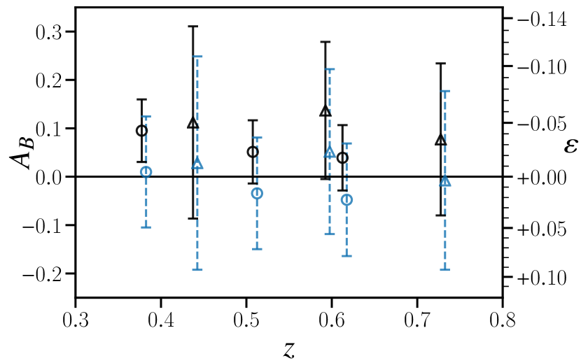
Figure 4: Marginal mean and standard deviation of $A_{B}$ as a function of redshift $z$ assuming $d_{\text{A}}$ values derived from Planck CPs. Results from the Planck and Planck-$w$CDM CPs are represented, respectively, by black (solid) and blue (dashed) bars. Similar to Figure 1, circles and triangles denote the result from SNIa + BOSS and SNIa + WiggleZ, respectively. On the right side, an alternative set of scales shows the same results expressed in terms of $\varepsilon$ as a proxy of systematics affecting BAO angular-diameter distances. The spacings on the $\varepsilon$ scale are logarithmic in $(1+\varepsilon)$, but within the relevant data range, they are visually indistinguishable from linear scales.

As we can see, the overall results are consistent with a null extinction magnitude, although there appears to be a slight preference of the sign, $A_{B}\geq 0$ (see Appendix A for a more detailed explanation).

The results described above constitute the main results for $A_{B}$ based on the Planck base CDM model that is precisely constrained by the CMB power spectra. To check whether an alternative dark energy prescription might modify our interpretation, we perform a similar analysis based on the Planck-$w$CDM cosmological posterior constraints.

It is worth noticing that a general problem with CMB constraints and non-CDM dark energy is parameter degeneracy. As the CMB spectral features are only indirectly sensitive to late-time evolution, free parameters introduced to describe more complex dark energy may not be well-constrained, and degeneracies may arise among parameters (see also Planck Collaboration, 2016b). In the case of $w$CDM, the Hubble constant $h$ fails to be constrained, as it is the case with KiDS posterior analysis. Therefore, we adopt the same re-weighting by the conservative Gaussian distribution (see Section 3.1). The inability to constrain $h$ has also be addressed by the Planck Collaboration (2016a, Section 5.4), and our re-weighting distribution is an update from their “conservative prior” based on Efstathiou (2014).

The results are displayed in tandem with the Planck base results in Table 3 and Figure 4. The use of re-weighted Planck-$w$CDM CP shifts $A_{B}$ closer to zero, but the standard deviation is about twice as large as the CDM one in the case of SNIa + BOSS even after re-weighting. The smaller sample size ($1.0\times 10^{4}$) also causes larger MC standard errors, but they remain dominated by the distributional spread. The shift results from the fact that $r_{\text{d}}$ (a parameter not directly affected by late-time dark energy) remains almost unchanged from the base CDM distribution, while the combination of $(h,\sqrt{\Omega_{\text{m}}})$ shifts along the direction of parameter degeneracy, shown in Figure 5. Overall, any evidence of deviation from $A_{B}=0$ is further weakened.

To compare with the earlier works, we cast the results in terms of the optical depth

$$\tau=\frac{(\ln 10)}{2.5}A_{B}=2\ln\eta$$ (7)

and take its redshift differential, thereby eliminating all dependence on the CPs. Using the SNIa + BOSS data set, we obtain $\tau(0.51)-\tau(0.38)=-0.04\pm 0.05$ and $\tau(0.61)-\tau(0.38)=-0.05\pm 0.05$. We have verified that these differentials, as expected, are essentially the same up to a small sampling error, independent of the CP choice. The uncertainties on $\Delta\tau$ are lower than in previous studies (More et al., 2009; Nair et al., 2012) by virtue of higher-precision distance data. Meanwhile, there is no conclusive support for evolving $\tau(z)$.

The generality of estimating relative increments in $\tau$ is gained at the cost of losing information about its amount in absolute terms. In contrast, our main $A_{B}$ estimates can be compared with independent estimations of intergalactic extinction. At $z=0.38$, we find our result broadly consistent with $A_{B}\approx 0.02$ reported by Ménard et al. (2010a, b) from $z\approx 0.36$ and other observational constraints cited therein.

These bounds are only one possible interpretation of cosmic distance systematics that induce apparent deviations from the DD relation. Should one uses the SNIa $d_{\text{L}}$ to access possible systematic shifts in BAO $d_{\text{A}}$, one would have used $\varepsilon=\eta^{-1}-1$ to express the increment by which the BAO-measured $d_{\text{A}}$ shifts relative to $d_{\text{L}}/(1+z)^{2}$, which we show as the right-side scale in Figure 4.

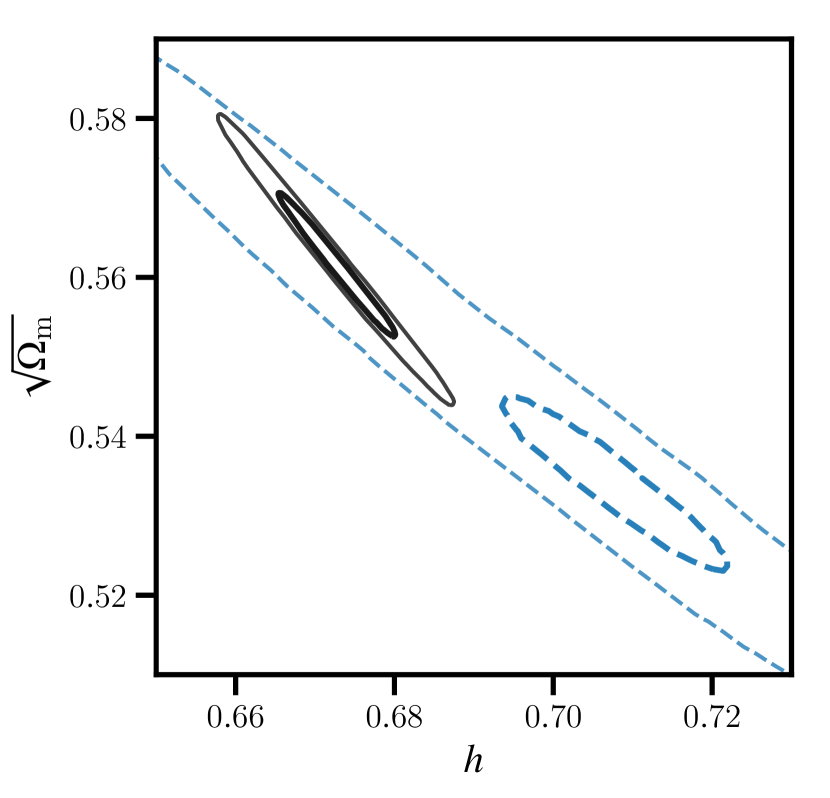
Figure 5: Shift of parameters $(h,\sqrt{\Omega_{\text{m}}})$ from Planck base CDM (solid, black) to $w$CDM (dashed, blue) posteriors, shown as $p_{1}=0.683$ and $p_{2}=0.954$ credible regions.

5 Discussion

In this work, we have performed DD relation tests using recent SNIa and BAO data. Assuming auxiliary cosmological information (i.e., CPs) that is necessary to obtain comparable $d_{\text{A}}$ and $d_{\text{L}}$ values, we find a 9% constraint consistent with $\eta=1$ from the analysis of SNIa + BOSS. The combination SNIa + WiggleZ is affected by greater statistical uncertainties in the BAO distances, but it allows us to probe a different redshift range, and we obtain qualitatively similar results with about 18% uncertainty in $\eta$.

Our results stand in contrast to earlier analyses using SNIa + clusters (e.g., Uzan et al., 2004; Holanda et al., 2010) or SNIa + BAO (e.g., Nair et al., 2012), in which $\eta<1$, or anomalous brightening, was reported as being close to or above $1\sigma$ level. We suspect the origin of their seemingly surprising conclusion might partially lie in the difference in the methods of statistical analysis.

The inclusion of tighter-bounded CPs, such as those from the Planck CDM CMB analysis, would lead to much tighter constraints on $\eta$ with about $3\%$ uncertainty. However, the Planck analysis assumes photon number conservation. Thus, Planck CPs cannot be used to test the DD relation directly. Nevertheless, such CPs can be combined with SNIa and BAO data to constrain systematic effects on cosmic distance measurements that manifest as an apparent deviation from the DD relation. In this work, we present examples of such analysis by inferring bounds on the SNIa extinction.We demonstrate the fact that such analysis dependents on high-precision cosmological posterior, while parameter degeneracy encountered with more complex dark energy models should be mitigated. In future studies, it will be worth exploring how the issue for precision may be approached in each context, especially in the presence of difficulty with combining cosmological information from independent probes in the context of extended dark energy models (see, e.g., Grandis et al., 2016).

The work presented here differs from previous analyses not only by the use of updated data but primarily by featuring new analysis methods.

The SNIa compression procedure (M16) produces accurate data covariance by properly treating the SNIa standardization uncertainties, in contrast to $\chi^{2}$ expressions found in similar studies (e.g., Liao et al., 2015) that would be inadequate for this task. Meanwhile, the method obviates the need to use narrow bands for redshift-matching. Compared with earlier approaches (e.g., More et al., 2009; Cardone et al., 2012; Rana et al., 2016), our compression is done in $\log_{10}z$ space where the systematic evolution of $\mu_{\text{L}}$ varies less nonlinearly, allowing us to use larger bandwidths. This reduces statistical uncertainties due to limited local sample size and is more robust against the systematics induced by a possibly nonrepresentative local sample. A similar method (Liang et al., 2013) was used with earlier Union2 SNIa data (Amanullah et al., 2010), but it did not share the aforementioned benefits and was not generalized to non-diagonal data covariance. Recently, a smoothing interpolation method based on Gaussian processes was applied to the analysis of DD relation (Rana et al., 2017), which could be used to reconstruct $\eta(z)$ as a smooth function. However, unlike in ours, in the aforementioned study (unlike ours), contribution to the final statistical distributions from SNIa standardization uncertainty was not accounted for.

Another advantage of our approach concerns the estimation of uncertainties on $\eta$. MC sampling allows us to directly propagate the probabilistic uncertainties of the data and the CP onto the distribution of $\eta$ or its functions consistently, without the need of assuming Gaussian uncertainties. In fact, not all of our results can be robustly approximated as Gaussian (see Appendix A). Our method can faithfully model the correlated uncertainties of $\eta$ estimations at different redshifts, which must be taken into account when investigating possible evolution of $\eta(z)$ or related quantities (see Section 4.2). To the authors’ knowledge, this is the first time the issue of cross-redshift correlation is explicitly demonstrated in similar studies.

Finally, unlike previous works, our test does not rely on parametric constraints of artificial $\eta(z)$ evolution templates. We indeed find that no such evolution could be convincingly indicated by current data. From the standpoint of statistical methodology, currently the availability of high-quality, independent, and matching $d_{\text{L}}$ and $d_{\text{A}}$ measurements is still scarce, thus not allowing many degrees of freedom for parametric fitting. Our attention thus focuses on the distributional properties of $\eta$ itself. We leave a parametric characterization of $\eta(z)$ to the future availability of abundant data.

In the future, surveys such as Euclid and LSST will increase the data sample size and improve the study of systematic effects in cosmic distance measurements, thereby allowing us to verify the DD relation with higher precision and accuracy. As an approximate evaluation, we assume the statistical uncertainty on $\mu_{\text{Lc}}$ scales as the inverse square root of SNIa sample size $N$, and that the uncertainties on BAO and WL $d_{\text{A}}$ at $z\approx 0.5$ remains at the current 1.4% level, a conservative estimate based on Euclid science objectives (Euclid Science Study Team, 2010, Section 3.1.1.2). Assuming further the current Planck CDM CPs and LSST SNIa “deep” sample size of $N\approx 10^{4}$ (LSST Science Collaboration, 2009, Section 11.2.2), we estimate the forecast statistical uncertainty on $\eta$ at $z\approx 0.5$ to be about 0.02, and about 0.04 mag on $A_{B}$, using mock data. It is worth pointing out that our method based on local compression of SNIa could be adapted to future large-sample SNIa surveys, while alternative methods based on individual SNIa selection or narrow-windowed local regression might exacerbate the effect of nonrepresentative subsamples (see Section 1). The high precision of future data may us provide us with more stringent validations of the DD relation or greater insight into the physical origin of any apparent violation thereof.

The data files and data-analysis programs used in this work are publicly available.

Appendix A Robustness of Gaussian Approximation for $A_{B}$ and $\eta$

We use the MC-estimated sample mean vectors and covariance matrices of $A_{B}$ obtained in Section 4.2 to approximate the CDM main results by the multivariate normal (MVN) distribution and study the robustness of the approximation with a graphical test. If a random sample with sample mean $\boldsymbol{\mu}$ and sample covariance $C$ is drawn from a $d$-dimensional MVN distribution, it follows that the sample of the square of the Mahalanobis distance from $\boldsymbol{\mu}$, defined as

$$l^{2}(\boldsymbol{x})=(\boldsymbol{x}-\boldsymbol{\mu})^{T}C^{-1}(\boldsymbol{x}-\boldsymbol{\mu}),$$ (A1)

has a beta distribution after scaling (Ververidis & Kotropoulos, 2008). Namely,

$$\frac{nl^{2}}{(n-1)^{2}}\sim\text{Beta}\left(\frac{d}{2},\frac{n-d-1}{2}\right).$$ (A2)

We plot the empirical quantiles of $nl^{2}/(n-1)^{2}$ against those of the theoretical distribution in Figure 6. Although both samples show deviations from the theoretical distribution only noticeably after about the 98th percentile, the tail distribution of the SNIa + BOSS sample behaves better than the one from SNIa + WiggleZ that shows considerable deviation.

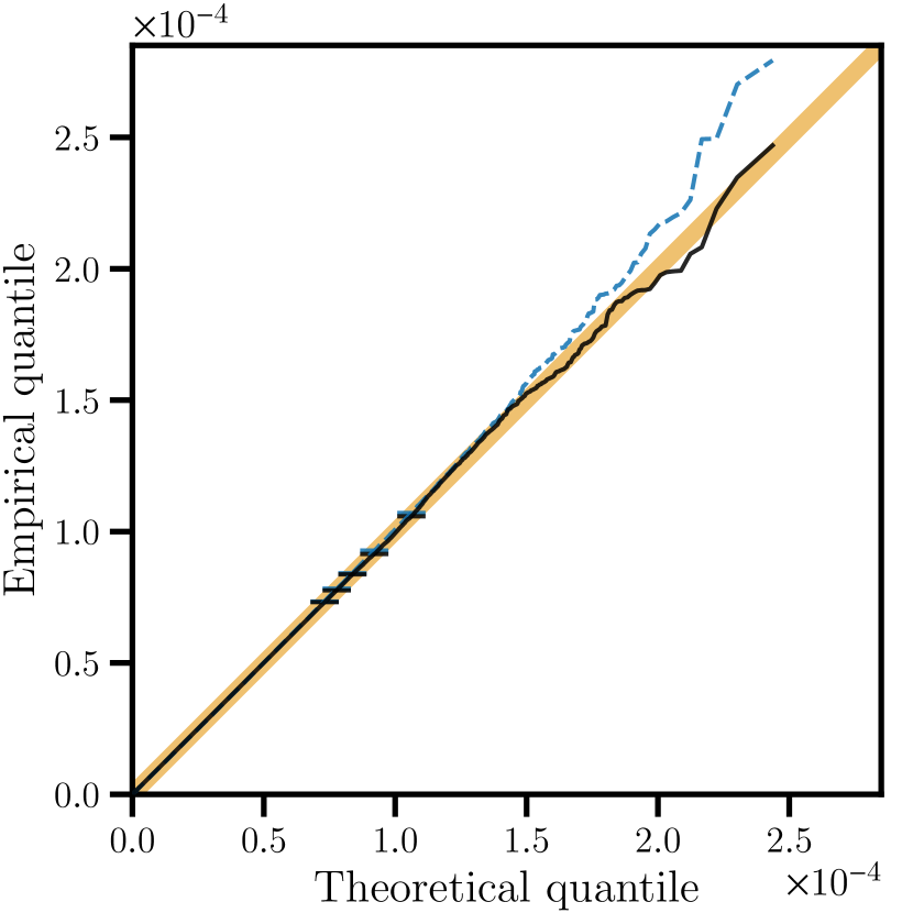
Figure 6: Q–Q plot of the squared Mahalanobis distance from the main $A_{B}$ samples versus the theoretical distribution assuming MVN. For readability, the line of equal distribution is displayed as an orange (shaded) band, and the data points (not shown) are connected by line segments. Markers show the positions of the 95th–99th percentiles. Results from SNIa + BOSS are shown in black (solid), and SNIa + WiggleZ in blue (dashed).

To understand these differences, we apply two complementary MVN tests, namely the empirical characteristic function test (Henze & Zirkler, 1990) with bandwidth parameter $\beta=0.5$ and the sample skewness test (Mardia, 1970). It should be noted that here we are not performing a hypothesis testing. Indeed, we already understand that MVN as a hypothesis is unlikely to be true: the distribution form of $A_{B}$ is manifestly non-Gaussian, and its MC generation is not an independent sampling process. Instead, we employ the former test’s sensitivity to heavy tails and the latter’s sensitivity to shape asymmetry to explain the deviations in Figure 6. The tests are applied to random subsamples of size $n=50$ and are repeated $10^{4}$ times. The rejection rates $r$ from the runs are compared with each other and with the significance level parameter $\alpha=0.05$. For SNIa + BOSS, Henze & Zirkler’s test produces $r=0.043$ and Mardia’s skewness test $r=0.040$. In contrast, for SNIa + WiggleZ both tests give $r=0.056$, in excess of $\alpha$.

The tests suggest the robustness of MVN approximation for $A_{B}$ from SNIa + BOSS, but not for the one from SNIa + WiggleZ that displays greater asymmetry and heavier tails. Therefore, we omit the approximation for the latter.

In future analysis, it may be necessary to factorize or invert the covariance matrix. For numerical stability, we increase the number of digits printed here, as presented in Table 4.

Table 4: Sample Mean and Covariance of $A_{B}$ from SNIa + BOSS with the Planck CP Set.

$z$	Mean	$\text{Covariance}\times 10^{3}$
0.38	0.0952	4.176680	2.817193	2.791656
0.51	0.0514	$\cdots$	4.259605	3.068827
0.61	0.0393	$\cdots$	$\cdots$	4.567452

Note. — To obtain the covariance matrix, multiply the values in the last three columns by $10^{-3}$.

We calculate the probability $p$ of $A_{B}(z)$ being positive at all the three redshifts given only the data, without model assumptions. This is the integral of the data PDF over the infinite cell (octant) where all of the coordinates are positive-valued. Numerical quadrature using MVN approximation finds $p\approx 0.64$. Direct MC integration using the $A_{B}$ sample produces essentially the same value, but its precision is limited by the MC sample size. We thus conclude that there is a slight preference of positive extinction (Section 4.2).

We also perform the three tests on the samples of $\eta$, and the results show substantial deviation from MVN in all cases.

References

- Abbott et al. (2017) Abbott, B. P., Abbott, R., Abbott, T. D., et al. 2017, Natur, 551, 85, doi: 10.1038/nature24471
- Alam et al. (2017) Alam, S., Ata, M., Bailey, S., et al. 2017, MNRAS, 470, 2617, doi: 10.1093/mnras/stx721
- Amanullah et al. (2010) Amanullah, R., Lidman, C., Rubin, D., et al. 2010, ApJ, 716, 712, doi: 10.1088/0004-637X/716/1/712
- Anderson et al. (2014) Anderson, L., Aubourg, É., Bailey, S., et al. 2014, MNRAS, 441, 24, doi: 10.1093/mnras/stu523
- Ballinger et al. (1996) Ballinger, W. E., Peacock, J. A., & Heavens, A. F. 1996, MNRAS, 282, 877, doi: 10.1093/mnras/282.3.877
- Bassett & Kunz (2004) Bassett, B. A., & Kunz, M. 2004, Phys. Rev. D, 69, 101305, doi: 10.1103/PhysRevD.69.101305
- Betoule et al. (2014) Betoule, M., Kessler, R., Guy, J., et al. 2014, A&A, 568, A22, doi: 10.1051/0004-6361/201423413
- Beutler et al. (2016) Beutler, F., Blake, C., Koda, J., et al. 2016, MNRAS, 455, 3230, doi: 10.1093/mnras/stv1943
- Blake et al. (2011a) Blake, C., Davis, T., Poole, G. B., et al. 2011a, MNRAS, 415, 2892, doi: 10.1111/j.1365-2966.2011.19077.x
- Blake et al. (2011b) Blake, C., Glazebrook, K., Davis, T. M., et al. 2011b, MNRAS, 418, 1725, doi: 10.1111/j.1365-2966.2011.19606.x
- Blake et al. (2012) Blake, C., Brough, S., Colless, M., et al. 2012, MNRAS, 425, 405, doi: 10.1111/j.1365-2966.2012.21473.x
- Bocquet et al. (2015) Bocquet, S., Saro, A., Mohr, J. J., et al. 2015, ApJ, 799, 214, doi: 10.1088/0004-637X/799/2/214
- Bonamente et al. (2006) Bonamente, M., Joy, M. K., LaRoque, S. J., et al. 2006, ApJ, 647, 25, doi: 10.1086/505291
- Cardone et al. (2012) Cardone, V. F., Spiro, S., Hook, I., & Scaramella, R. 2012, Phys. Rev. D, 85, 123510, doi: 10.1103/PhysRevD.85.123510
- Chiu et al. (2016) Chiu, I., Mohr, J., McDonald, M., et al. 2016, MNRAS, 455, 258, doi: 10.1093/mnras/stv2303
- Chluba (2014) Chluba, J. 2014, MNRAS, 443, 1881, doi: 10.1093/mnras/stu1260
- Corasaniti (2006) Corasaniti, P.-S. 2006, MNRAS, 372, 191, doi: 10.1111/j.1365-2966.2006.10825.x
- Crocce & Scoccimarro (2008) Crocce, M., & Scoccimarro, R. 2008, Phys. Rev. D, 77, 023533, doi: 10.1103/PhysRevD.77.023533
- Cyburt et al. (2016) Cyburt, R. H., Fields, B. D., Olive, K. A., & Yeh, T.-H. 2016, RvMP, 88, 015004, doi: 10.1103/RevModPhys.88.015004
- De Bernardis et al. (2006) De Bernardis, F., Giusarma, E., & Melchiorri, A. 2006, IJMPD, 15, 759, doi: 10.1142/S0218271806008486
- Droettboom et al. (2018) Droettboom, M., Hunter, J., Caswell, T. A., et al. 2018, matplotlib, 2.2.2, Zenodo, doi: 10.5281/zenodo.1202077. https://doi.org/10.5281/zenodo.1202077
- Efstathiou (2014) Efstathiou, G. 2014, MNRAS, 440, 1138, doi: 10.1093/mnras/stu278
- Eisenstein et al. (2005) Eisenstein, D. J., Zehavi, I., Hogg, D. W., et al. 2005, ApJ, 633, 560, doi: 10.1086/466512
- Ellis (1971) Ellis, G. F. R. 1971, in Proceedings of the International School of Physics “Enrico Fermi”, Course 47: General Relativity and Cosmology, ed. R. K. Sachs (New York, US: Academic Press), 104–182
- Ellis (2009) Ellis, G. F. R. 2009, GReGr, 41, 581, doi: 10.1007/s10714-009-0760-7
- Etherington (1933) Etherington, I. M. H. 1933, PMag, 7, 761
- Etherington (2007) —. 2007, GReGr, 39, 1055, doi: 10.1007/s10714-007-0447-x
- Euclid Science Study Team (2010) Euclid Science Study Team. 2010, Euclid Science Requirements Document, Tech. Rep. DEM-SA-Dc-00001, European Space Research and Technology Centre, ESA, Noordwijk, NL
- Evslin (2016) Evslin, J. 2016, PDU, 14, 57, doi: 10.1016/j.dark.2016.09.005
- Flegal et al. (2008) Flegal, J. M., Haran, M., & Jones, G. L. 2008, StatSc, 23, 250, doi: 10.1214/08-STS257
- Fu & Li (2017) Fu, X., & Li, P. 2017, IJMPD, 26, 1750097, doi: 10.1142/S0218271817500973
- Gonzalez et al. (2013) Gonzalez, A. H., Sivanandam, S., Zabludoff, A. I., & Zaritsky, D. 2013, ApJ, 778, 14, doi: 10.1088/0004-637X/778/1/14
- Goobar & Leibundgut (2011) Goobar, A., & Leibundgut, B. 2011, ARNPS, 61, 251, doi: 10.1146/annurev-nucl-102010-130434
- Grandis et al. (2016) Grandis, S., Rapetti, D., Saro, A., Mohr, J. J., & Dietrich, J. P. 2016, MNRAS, 463, 1416, doi: 10.1093/mnras/stw2028
- Henze & Zirkler (1990) Henze, N., & Zirkler, B. 1990, Commun. Stat., Theory Methods, 19, 3595, doi: 10.1080/03610929008830400
- Hildebrandt et al. (2017) Hildebrandt, H., Viola, M., Heymans, C., et al. 2017, MNRAS, 465, 1454, doi: 10.1093/mnras/stw2805
- Holanda et al. (2016) Holanda, R. F. L., Busti, V. C., & Alcaniz, J. S. 2016, J. Cosmology Astropart. Phys, 2, 054, doi: 10.1088/1475-7516/2016/02/054
- Holanda et al. (2017) Holanda, R. F. L., Busti, V. C., Lima, F. S., & Alcaniz, J. S. 2017, J. Cosmology Astropart. Phys, 9, 039, doi: 10.1088/1475-7516/2017/09/039
- Holanda et al. (2010) Holanda, R. F. L., Lima, J. A. S., & Ribeiro, M. B. 2010, ApJ, 722, L233, doi: 10.1088/2041-8205/722/2/L233
- Hu et al. (1995) Hu, W., Scott, D., Sugiyama, N., & White, M. 1995, Phys. Rev. D, 52, 5498, doi: 10.1103/PhysRevD.52.5498
- Hunter (2007) Hunter, J. D. 2007, CSE, 9, 90, doi: 10.1109/MCSE.2007.55
- Lewis et al. (2000) Lewis, A., Challinor, A., & Lasenby, A. 2000, ApJ, 538, 473, doi: 10.1086/309179
- Lewis et al. (2017) Lewis, A., Mead, A., Vehreschild, A., et al. 2017, CAMB, August 2017, doi: 10.5281/zenodo.844843
- Liang et al. (2013) Liang, N., Li, Z., Wu, P., et al. 2013, MNRAS, 436, 1017, doi: 10.1093/mnras/stt1589
- Liao et al. (2015) Liao, K., Avgoustidis, A., & Li, Z. 2015, Phys. Rev. D, 92, 123539, doi: 10.1103/PhysRevD.92.123539
- Liao et al. (2016) Liao, K., Li, Z., Cao, S., et al. 2016, ApJ, 822, 74, doi: 10.3847/0004-637X/822/2/74
- LSST Science Collaboration (2009) LSST Science Collaboration. 2009, preprint. https://arxiv.org/abs/0912.0201
- Ma et al. (2016) Ma, C., Corasaniti, P.-S., & Bassett, B. A. 2016, MNRAS, 463, 1651, doi: 10.1093/mnras/stw2069
- Mardia (1970) Mardia, K. V. 1970, Biometrika, 57, 519, doi: 10.1093/biomet/57.3.519
- Max-Moerbeck et al. (2014) Max-Moerbeck, W., Richards, J. L., Hovatta, T., et al. 2014, MNRAS, 445, 437, doi: 10.1093/mnras/stu1707
- Mehta et al. (2012) Mehta, K. T., Cuesta, A. J., Xu, X., Eisenstein, D. J., & Padmanabhan, N. 2012, MNRAS, 427, 2168, doi: 10.1111/j.1365-2966.2012.21112.x
- Ménard et al. (2010a) Ménard, B., Kilbinger, M., & Scranton, R. 2010a, MNRAS, 406, 1815, doi: 10.1111/j.1365-2966.2010.16464.x
- Ménard et al. (2010b) Ménard, B., Scranton, R., Fukugita, M., & Richards, G. 2010b, MNRAS, 405, 1025, doi: 10.1111/j.1365-2966.2010.16486.x
- Meng et al. (2012) Meng, X.-L., Zhang, T.-J., Zhan, H., & Wang, X. 2012, ApJ, 745, 98, doi: 10.1088/0004-637X/745/1/98
- More et al. (2009) More, S., Bovy, J., & Hogg, D. W. 2009, ApJ, 696, 1727, doi: 10.1088/0004-637X/696/2/1727
- Nair et al. (2012) Nair, R., Jhingan, S., & Jain, D. 2012, J. Cosmology Astropart. Phys, 12, 028, doi: 10.1088/1475-7516/2012/12/028
- Planck Collaboration (2016a) Planck Collaboration. 2016a, A&A, 594, A13, doi: 10.1051/0004-6361/201525830
- Planck Collaboration (2016b) —. 2016b, A&A, 594, A14, doi: 10.1051/0004-6361/201525814
- Rana et al. (2016) Rana, A., Jain, D., Mahajan, S., & Mukherjee, A. 2016, J. Cosmology Astropart. Phys, 7, 026, doi: 10.1088/1475-7516/2016/07/026
- Rana et al. (2017) Rana, A., Jain, D., Mahajan, S., Mukherjee, A., & Holanda, R. F. L. 2017, J. Cosmology Astropart. Phys, 7, 010, doi: 10.1088/1475-7516/2017/07/010
- Räsänen et al. (2016) Räsänen, S., Väliviita, J., & Kosonen, V. 2016, J. Cosmology Astropart. Phys, 4, 050, doi: 10.1088/1475-7516/2016/04/050
- Rasera et al. (2014) Rasera, Y., Corasaniti, P.-S., Alimi, J.-M., et al. 2014, MNRAS, 440, 1420, doi: 10.1093/mnras/stu295
- Riess et al. (2016) Riess, A. G., Macri, L. M., Hoffmann, S. L., et al. 2016, ApJ, 826, 56, doi: 10.3847/0004-637X/826/1/56
- Riess et al. (2018) Riess, A. G., Casertano, S., Yuan, W., et al. 2018, ApJ, 855, 136, doi: 10.3847/1538-4357/aaadb7
- Rigault et al. (2015) Rigault, M., Aldering, G., Kowalski, M., et al. 2015, ApJ, 802, 20, doi: 10.1088/0004-637X/802/1/20
- Santos-da-Costa et al. (2015) Santos-da-Costa, S., Busti, V. C., & Holanda, R. F. L. 2015, J. Cosmology Astropart. Phys, 10, 061, doi: 10.1088/1475-7516/2015/10/061
- Schneider & Sluse (2013) Schneider, P., & Sluse, D. 2013, A&A, 559, A37, doi: 10.1051/0004-6361/201321882
- Seabold et al. (2017) Seabold, S., Perktold, J., Fulton, C., et al. 2017, statsmodels, 0.8.0, Zenodo, doi: 10.5281/zenodo.275519
- Seager et al. (2000) Seager, S., Sasselov, D. D., & Scott, D. 2000, ApJS, 128, 407, doi: 10.1086/313388
- Uzan et al. (2004) Uzan, J.-P., Aghanim, N., & Mellier, Y. 2004, Phys. Rev. D, 70, 083533, doi: 10.1103/PhysRevD.70.083533
- Ververidis & Kotropoulos (2008) Ververidis, D., & Kotropoulos, C. 2008, ITSP, 56, 2797, doi: 10.1109/TSP.2008.917350
- Wu et al. (2015) Wu, P., Li, Z., Liu, X., & Yu, H. 2015, Phys. Rev. D, 92, 023520, doi: 10.1103/PhysRevD.92.023520
- Yang et al. (2013) Yang, X., Yu, H.-R., Zhang, Z.-S., & Zhang, T.-J. 2013, ApJ, 777, L24, doi: 10.1088/2041-8205/777/2/L24