Mathematical Analysis of Ultrafast Ultrasound Imaging

Giovanni S. Alberti Department of Mathematics, ETH Zürich, Rämistrasse 101, 8092 Zürich, Switzerland (giovanni.alberti@math.ethz.ch, habib.ammari@math.ethz.ch, francisco.romero@sam.math.ethz.ch).    Habib Ammari11footnotemark: 1    Francisco Romero11footnotemark: 1    Timothée Wintz Department of Mathematics and Applications, École Normale Supérieure, 45 Rue d’Ulm, 75005 Paris, France (timothee.wintz@ens.fr).
(September 28, 2016)
Abstract

This paper provides a mathematical analysis of ultrafast ultrasound imaging. This newly emerging modality for biomedical imaging uses plane waves instead of focused waves in order to achieve very high frame rates. We derive the point spread function of the system in the Born approximation for wave propagation and study its properties. We consider dynamic data for blood flow imaging, and introduce a suitable random model for blood cells. We show that a singular value decomposition method can successfully remove the clutter signal by using the different spatial coherence of tissue and blood signals, thereby providing high-resolution images of blood vessels, even in cases when the clutter and blood speeds are comparable in magnitude. Several numerical simulations are presented to illustrate and validate the approach.

Key words. Ultrafast ultrasound imaging, singular value decomposition, Casorati matrix, blood flow imaging.

Mathematics Subject Classification. 65Z05, 74J25, 35R30.

1 Introduction

Conventional ultrasound imaging is performed with focused ultrasonic waves [18, 17]. This yields relatively good spatial resolution, but clearly limits the acquisition time, since the entire specimen has to be scanned. Over the last decade, ultrafast imaging in biomedical ultrasound has been developed [16, 19, 8]. Plane waves are used instead of focused waves, thereby limiting the resolution but increasing the frame rate considerably, up to 20,000 frames per second. Ultrafast imaging has been made possible by the recent technological advances in ultrasonic transducers, but the idea of ultrafast ultrasonography dates back to 1977 [5]. The advantages given by the very high frame rate are many, and the applications of this new modality range from blood flow imaging [2, 8], deep superresolution vascular imaging [9] and functional imaging of the brain [14, 15] to ultrasound elastography [10]. In this paper we focus on blood flow imaging.

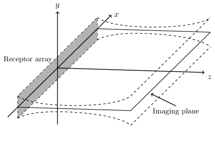
A single ultrafast ultrasonic image is obtained as follows [16]. A pulsed plane wave (focused on the imaging plane – see Figure 1b) insonifies the medium, and the back-scattered echoes are measured at the receptor array, a linear array of piezoelectric transducers. These spatio-temporal measurements are then beamformed to obtain a two-dimensional spatial signal. This is what we call static inverse problem, as it involves only a single wave, and the dynamics of the medium is not captured. The above procedure yields very low lateral resolution, i.e. in the direction parallel to the wavefront, because of the absence of focusing. In order to solve this issue, it was proposed to use multiple waves with different angles: these improve the lateral resolution, but has the drawback of reducing the frame rate.

For dynamic imaging, the above process is repeated many times, which gives several thousand images per second. In blood flow imaging, we are interested in locating blood vessels. One of the main issues lies in the removal of the clutter signal, typically the signal scattered from tissues, as it introduces major artifacts [3]. Ultrafast ultrasonography allows to overcome this issue, thanks to the very high frame rate. Temporal filters [2, 14, 15], based on high-pass filtering the data to remove clutter signals, have shown limited success in cases when the clutter and blood velocities are close (typically of the order of 102ms1superscript102msuperscripts110^{-2}\,\mathrm{m\!\cdot\!s^{-1}}), or even if the blood velocity is smaller than the clutter velocity. A spatio-temporal method based on the singular value decomposition (SVD) of the data was proposed in [8] to overcome this drawback, by exploiting the different spatial coherence of clutter and blood scatterers. Spatial coherence is understood as similar movement, in direction and speed, in large parts of the imaged zone. Tissue behaves with higher spatial coherence when compared to the blood flow, since large parts of the medium typically move in the same way, while blood flow is concentrated only in small vessels, which do not share necessarily the same movement direction and speed. This explains why spatial properties are crucial to perform the separation.

In this work, we provide a detailed mathematical analysis of ultrasound ultrafast imaging. To our knowledge, this is the first mathematical paper addressing the important challenges of this emerging and very promising modality. Even though in this work we limit ourselves to formalize the existing methods, the mathematical analysis provided gives important insights, which we expect will lead to improved reconstruction schemes.

The contributions of this paper are twofold. First, we carefully study the forward and inverse static problems. In particular, we derive the point spread function (PSF) of the system, in the Born approximation for ultrasonic wave propagation. We investigate the behavior of the PSF, and analyze the advantages of angle compounding. In particular, we study the lateral and vertical resolutions. In addition, this analysis allows us to fully understand the roles of the key parameters of the system, such as the directivity of the array and the settings related to angle compounding.

Second, we consider the dynamic problem. The analysis of the PSF provided allows to study the doppler effect, describing the dependence on the direction of the flow. Moreover, we consider a random model for the movement of blood cells, which allows us to study and justify the SVD method for the separation of the blood signal from the clutter signal, leading to the reconstruction of the blood vessels’ geometry. The analysis is based on the empirical study of the distribution of the singular values, which follows from the statistical properties of the relative data. We provide extensive numerical simulations, which illustrate and validate this approach.

This paper is structured as follows. In Section 2 we describe the imaging system and the model for wave propagation. In Section 3 we discuss the static inverse problem. In particular, we describe the beamforming process, the PSF and the angle compounding technique. In Section 4 the dynamic forward problem is considered: we briefly discuss how the dynamic data are obtained and analyze the doppler effect. In Section 5 we focus on the source separation to solve the dynamic inverse problem. We discuss the random model for the refractive index and the method based on the SVD decomposition of the data. In Section 6 numerical experiments are provided. Some concluding remarks and outlooks are presented in the final section.

2 The Static Forward Problem

The imaging system is composed of a medium contained in +3:={(x,y,z)3:z>0}assignsuperscriptsubscript3conditional-set𝑥𝑦𝑧superscript3𝑧0\mathbb{R}_{+}^{3}:=\{(x,y,z)\in\mathbb{R}^{3}:z>0\} and of a fixed linear array of transducers located on the line z=0,y=0formulae-sequence𝑧0𝑦0z=0,y=0. This linear array of piezoelectric transducers (see [18, Chapter 7]) produces an acoustic illumination that is focused in elevation – in the y𝑦y coordinates, near the plane y=0𝑦0y=0 – and has the form of a plane wave in the direction 𝐤S1𝐤superscript𝑆1\mathbf{k}\in S^{1} in the x,z𝑥𝑧x,z coordinates (see Figure 1b). Typical sizes for the array length and for the penetration depth are about 101msuperscript101m10^{-1}\,\mathrm{m}.

We make the assumption that the acoustic incident field uisuperscript𝑢𝑖u^{i} can be approximated as

ui(x,y,z,t)=Az(y)f(tc01𝐤(x,z)),superscript𝑢𝑖𝑥𝑦𝑧𝑡subscript𝐴𝑧𝑦𝑓𝑡superscriptsubscript𝑐01𝐤𝑥𝑧u^{i}\left(x,y,z,t\right)=A_{z}\left(y\right)f\left(t-c_{0}^{-1}\mathbf{k}\cdot\left(x,z\right)\right),

where c0subscript𝑐0c_{0} is the background speed of sound in the medium. The function Azsubscript𝐴𝑧A_{z} describes the beam waist in the elevation direction at depth z𝑧z (between 4103m4superscript103m4\cdot 10^{-3}\,\mathrm{m} and 102msuperscript102m10^{-2}\,\mathrm{m}). This is a simplified expression of the true incoming wave, which is focused by a cylindrical acoustic lens located near the receptor array (see [18, Chapters 6 and 7]). The function f𝑓f is the waveform describing the shape of the input pulse:

f(t)=e2πiν0tχ(ν0t),χ(u)=eu2τ2,formulae-sequence𝑓𝑡superscript𝑒2𝜋𝑖subscript𝜈0𝑡𝜒subscript𝜈0𝑡𝜒𝑢superscript𝑒superscript𝑢2superscript𝜏2f(t)=e^{2\pi i\nu_{0}t}\chi\left(\nu_{0}t\right),\qquad\chi\left(u\right)=e^{-\frac{u^{2}}{\tau^{2}}}, (1)

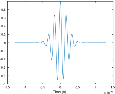
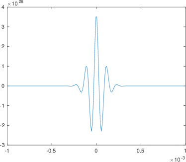
where ν0subscript𝜈0\nu_{0} is the principal frequency and τ𝜏\tau the width parameter of the pulse (see Figure 1a). Typically, ν0subscript𝜈0\nu_{0} will be of the order of 106s1superscript106superscripts110^{6}\,\mathrm{s^{-1}}. More precisely, realistic quantities are

c0=1.5103ms1,ν0=6106s1,τ=1.formulae-sequencesubscript𝑐01.5superscript103msuperscripts1formulae-sequencesubscript𝜈06superscript106superscripts1𝜏1c_{0}=1.5\cdot 10^{3}\,\mathrm{m\!\cdot\!s^{-1}},\quad\nu_{0}=6\cdot 10^{6}\,\mathrm{s^{-1}},\quad\tau=1. (2)
Refer to caption
(a) The real part of the input pulse f𝑓f.
Refer to caption
(b) The imaging system. The incident wave is supported near the imaging plane {y=0}𝑦0\{y=0\}, within the focusing region bounded by the two curved surfaces.
Figure 1: The pulse f𝑓f of the incident wave uisuperscript𝑢𝑖u^{i} and the focusing region.

Let c:3+:𝑐superscript3subscriptc:\mathbb{R}^{3}\rightarrow\mathbb{R}_{+} be the speed of sound and consider the perturbation n𝑛n given by

n(𝐱)=1c2(𝐱)1c02.𝑛𝐱1superscript𝑐2𝐱1superscriptsubscript𝑐02n\left(\mathbf{x}\right)=\frac{1}{c^{2}\left(\mathbf{x}\right)}-\frac{1}{c_{0}^{2}}.

We assume that suppn+3supp𝑛subscriptsuperscript3\mbox{supp}\,n\subseteq\mathbb{R}^{3}_{+}. The acoustic pressure in the medium satisfies the wave equation

Δu(𝐱,t)1c2(𝐱)2t2u(𝐱,t)=0,𝐱3,formulae-sequenceΔ𝑢𝐱𝑡1superscript𝑐2𝐱superscript2superscript𝑡2𝑢𝐱𝑡0𝐱superscript3\Delta u\left(\mathbf{x},t\right)-\frac{1}{c^{2}\left(\mathbf{x}\right)}\frac{\partial^{2}}{\partial t^{2}}u\left(\mathbf{x},t\right)=0,\qquad\mathbf{x}\in\mathbb{R}^{3},

with a suitable radiation condition on uui𝑢superscript𝑢𝑖u-u^{i}. Let G𝐺G denote the Green’s function for the acoustic wave equation in 3superscript3\mathbb{R}^{3} [1, 20]:

G(𝐱,t,𝐱,t)=(4π)1|𝐱𝐱|δ((tt)c01|𝐱𝐱|).𝐺𝐱𝑡superscript𝐱superscript𝑡superscript4𝜋1𝐱superscript𝐱𝛿𝑡superscript𝑡superscriptsubscript𝑐01𝐱superscript𝐱G(\mathbf{x},t,\mathbf{x}^{\prime},t^{\prime})=-\frac{(4\pi)^{-1}}{\left|\mathbf{x}-\mathbf{x}^{\prime}\right|}\delta\left(\left(t-t^{\prime}\right)-c_{0}^{-1}\left|\mathbf{x}-\mathbf{x}^{\prime}\right|\right).

In the following, we will assume that the Born approximation holds, i.e. we consider only first reflections on scatterers, and neglect subsequent reflections [1, 7] (in cases when the Born approximation is not valid, nonlinear methods have to be used). This is a very common approximation in medical imaging, and is justified by the fact that soft biological tissues are almost acoustic homogeneous, due to the high water concentration. In mathematical terms, it consists in the linearization around the constant sound speed c0subscript𝑐0c_{0}. In this case, the scattered wave us:=uuiassignsuperscript𝑢𝑠𝑢superscript𝑢𝑖u^{s}:=u-u^{i} is given by

us(𝐱,t)=3n(𝐱)2uit2(𝐱,t)G(𝐱,t,𝐱,t)𝑑𝐱𝑑t,𝐱3,t+,formulae-sequencesuperscript𝑢𝑠𝐱𝑡subscriptsubscriptsuperscript3𝑛superscript𝐱superscript2superscript𝑢𝑖superscript𝑡2superscript𝐱superscript𝑡𝐺𝐱𝑡superscript𝐱superscript𝑡differential-dsuperscript𝐱differential-dsuperscript𝑡formulae-sequence𝐱superscript3𝑡subscriptu^{s}\left(\mathbf{x},t\right)=\int_{\mathbb{R}}\int_{\mathbb{R}^{3}}n\left(\mathbf{x}^{\prime}\right)\frac{\partial^{2}u^{i}}{\partial t^{2}}\left(\mathbf{x}^{\prime},t^{\prime}\right)G\left(\mathbf{x},t,\mathbf{x}^{\prime},t^{\prime}\right)d\mathbf{x}^{\prime}dt^{\prime},\qquad\mathbf{x}\in\mathbb{R}^{3},\;t\in\mathbb{R}_{+},

since contributions from nt2us𝑛superscriptsubscript𝑡2superscript𝑢𝑠n\partial_{t}^{2}u^{s} are negligible. Therefore, inserting the expressions for the Green’s function and for the incident wave yields

us(𝐱,t)=3(4π)1|𝐱𝐱|n(𝐱)Az(y)f′′(tc01((x,z)𝐤+|𝐱𝐱|))𝑑𝐱,superscript𝑢𝑠𝐱𝑡subscriptsuperscript3superscript4𝜋1𝐱superscript𝐱𝑛superscript𝐱subscript𝐴superscript𝑧superscript𝑦superscript𝑓′′𝑡superscriptsubscript𝑐01superscript𝑥superscript𝑧𝐤𝐱superscript𝐱differential-dsuperscript𝐱u^{s}\left(\mathbf{x},t\right)=-\int_{\mathbb{R}^{3}}\frac{(4\pi)^{-1}}{\left|\mathbf{x}-\mathbf{x}^{\prime}\right|}n\left(\mathbf{x}^{\prime}\right)A_{z^{\prime}}\left(y^{\prime}\right)f^{\prime\prime}\left(t-c_{0}^{-1}\left((x^{\prime},z^{\prime})\cdot\mathbf{k}+\left|\mathbf{x}-\mathbf{x}^{\prime}\right|\right)\right)d\mathbf{x}^{\prime},

where we set 𝐱=(x,y,z)𝐱𝑥𝑦𝑧\mathbf{x}=(x,y,z) and 𝐱=(x,y,z)superscript𝐱superscript𝑥superscript𝑦superscript𝑧\mathbf{x}^{\prime}=(x^{\prime},y^{\prime},z^{\prime}). Since the waist of the beam in the y𝑦y direction is small compared to the distance at which we image the medium, we can make the assumption

|𝐱(x,y,z)||𝐱(x,0,z)|,𝐱=(x,0,0)3,formulae-sequencesimilar-to-or-equals𝐱superscript𝑥superscript𝑦superscript𝑧𝐱superscript𝑥0superscript𝑧𝐱𝑥00superscript3\left|\mathbf{x}-\left(x^{\prime},y^{\prime},z^{\prime}\right)\right|\simeq\left|\mathbf{x}-\left(x^{\prime},0,z^{\prime}\right)\right|,\qquad\mathbf{x}=\left(x,0,0\right)\in\mathbb{R}^{3},

so that the following expression for ussuperscript𝑢𝑠u^{s} holds for 𝐱=(x,0,0)3𝐱𝑥00superscript3\mathbf{x}=\left(x,0,0\right)\in\mathbb{R}^{3} and t>0𝑡0t>0:

us(𝐱,t)=2(4π)1|𝐱(x,0,z)|f′′(tc01((x,z)𝐤+|𝐱(x,0,z)|))n~(x,z)𝑑x𝑑z,superscript𝑢𝑠𝐱𝑡subscriptsuperscript2superscript4𝜋1𝐱superscript𝑥0superscript𝑧superscript𝑓′′𝑡superscriptsubscript𝑐01superscript𝑥superscript𝑧𝐤𝐱superscript𝑥0superscript𝑧~𝑛superscript𝑥superscript𝑧differential-dsuperscript𝑥differential-dsuperscript𝑧u^{s}\left(\mathbf{x},t\right)\!=\!\int_{\mathbb{R}^{2}}\frac{-(4\pi)^{-1}}{\left|\mathbf{x}-\left(x^{\prime},0,z^{\prime}\right)\right|}f^{\prime\prime}\left(t-c_{0}^{-1}\left((x^{\prime},z^{\prime})\cdot\mathbf{k}+\left|\mathbf{x}-\left(x^{\prime},0,z^{\prime}\right)\right|\right)\right)\tilde{n}(x^{\prime},z^{\prime})dx^{\prime}dz^{\prime},

where n~~𝑛\tilde{n} is given by

n~(x,z):=n(𝐱)Az(y)𝑑y,𝐱=(x,y,z)3.formulae-sequenceassign~𝑛superscript𝑥superscript𝑧subscript𝑛superscript𝐱subscript𝐴superscript𝑧superscript𝑦differential-dsuperscript𝑦superscript𝐱superscript𝑥superscript𝑦superscript𝑧superscript3\tilde{n}(x^{\prime},z^{\prime}):=\int_{\mathbb{R}}n\left(\mathbf{x^{\prime}}\right)A_{z^{\prime}}\left(y^{\prime}\right)dy^{\prime},\qquad\mathbf{x}^{\prime}=(x^{\prime},y^{\prime},z^{\prime})\in\mathbb{R}^{3}. (3)

Since our measurements are only two-dimensional (one spatial dimension given by the linear array and one temporal dimension), we cannot aim to reconstruct the full three-dimensional refractive index n𝑛n. However, the above identity provides a natural expression for what can be reconstructed: the vertical averages n~~𝑛\tilde{n} of n𝑛n. Since Azsubscript𝐴𝑧A_{z} is supported near y=0𝑦0y=0, n~~𝑛\tilde{n} reflects the contribution of n𝑛n only near the imaging plane. In physical terms, n~~𝑛\tilde{n} contains all the scatterers in the support of Azsubscript𝐴𝑧A_{z}; these scatterers are in some sense projected onto y=0𝑦0y=0, the imaging plane. For simplicity, with an abuse of notation from now on we shall simply denote n~~𝑛\tilde{n} by n𝑛n, since the original three-dimensional n𝑛n will not play any role, due to the dimensionality restriction discussed above. Moreover, for the same reasons, all vectors 𝐱𝐱\mathbf{x} and 𝐱superscript𝐱\mathbf{x}^{\prime} will be two-dimensional, namely, 𝐱=(x,z)𝐱𝑥𝑧\mathbf{x}=(x,z) and similarly for 𝐱superscript𝐱\mathbf{x}^{\prime}. In view of these considerations, for 𝐱=(x,0)2𝐱𝑥0superscript2\mathbf{x}=(x,0)\in\mathbb{R}^{2} and t>0𝑡0t>0 the scattering wave takes the form

us(𝐱,t)=2(4π)1|𝐱𝐱|f′′(tc01(𝐱𝐤+|𝐱𝐱|))n(𝐱)𝑑𝐱.superscript𝑢𝑠𝐱𝑡subscriptsuperscript2superscript4𝜋1𝐱superscript𝐱superscript𝑓′′𝑡superscriptsubscript𝑐01superscript𝐱𝐤𝐱superscript𝐱𝑛superscript𝐱differential-dsuperscript𝐱u^{s}\left(\mathbf{x},t\right)=-\int_{\mathbb{R}^{2}}\frac{(4\pi)^{-1}}{\left|\mathbf{x}-\mathbf{x}^{\prime}\right|}f^{\prime\prime}\left(t-c_{0}^{-1}\left(\mathbf{x}^{\prime}\cdot\mathbf{k}+\left|\mathbf{x}-\mathbf{x}^{\prime}\right|\right)\right)n\left(\mathbf{x}^{\prime}\right)d\mathbf{x}^{\prime}. (4)

It is useful to parametrize the direction 𝐤S1𝐤superscript𝑆1{\bf k}\in S^{1} of the incident wave by 𝐤=𝐤θ=(sinθ,cosθ)𝐤subscript𝐤𝜃𝜃𝜃{\bf k}={\bf k}_{\theta}=(\sin\theta,\cos\theta) for some θ𝜃\theta\in\mathbb{R}; in practice, |θ|0.25𝜃0.25|\theta|\leq 0.25 [16].

3 The Static Inverse Problem

The static inverse problem consists in the reconstruction of n𝑛n (up to a convolution kernel) from the measurements ussuperscript𝑢𝑠u^{s} at the receptors, assuming that n𝑛n does not depend on time. This process provides a single image, and will be repeated many times in order to obtain dynamic imaging, as it is discussed in the next sections.

3.1 Beamforming

The receptor array is a segment Γ=(A,A)×{0}Γ𝐴𝐴0\Gamma=\left(-A,A\right)\times\left\{0\right\} for some A>0𝐴0A>0. The travel time from the receptor array to a point 𝐱=(x,z)𝐱𝑥𝑧\mathbf{x}=\left(x,z\right) and back to a receptor located in 𝐮0=(u,0)subscript𝐮0𝑢0\mathbf{u}_{0}=\left(u,0\right) is given by

τ𝐱θ(u)=c01(𝐱𝐤θ+|𝐱𝐮0|).superscriptsubscript𝜏𝐱𝜃𝑢superscriptsubscript𝑐01𝐱subscript𝐤𝜃𝐱subscript𝐮0\tau_{\mathbf{x}}^{\theta}\left(u\right)=c_{0}^{-1}\left(\mathbf{x}\cdot\mathbf{k}_{\theta}+\left|\mathbf{x}-{\bf u}_{0}\right|\right).

The beamforming process [18, 16] consists in averaging the measured signals on ΓΓ\Gamma at t=τ𝐱θ(u)𝑡superscriptsubscript𝜏𝐱𝜃𝑢t=\tau_{\mathbf{x}}^{\theta}\left(u\right), which results in the image

sθ(x,z):=xFzx+Fzus(𝐮0,τ𝐱θ(u))𝑑u,𝐱=(x,z)+2:={(x,z)2:z>0}.formulae-sequenceassignsubscript𝑠𝜃𝑥𝑧superscriptsubscript𝑥𝐹𝑧𝑥𝐹𝑧superscript𝑢𝑠subscript𝐮0superscriptsubscript𝜏𝐱𝜃𝑢differential-d𝑢𝐱𝑥𝑧superscriptsubscript2assignconditional-set𝑥𝑧superscript2𝑧0s_{\theta}(x,z):=\int_{x-Fz}^{x+Fz}u^{s}\left(\mathbf{u}_{0},\tau_{\mathbf{x}}^{\theta}\left(u\right)\right)du,\qquad\mathbf{x}=(x,z)\in\mathbb{R}_{+}^{2}:=\{(x,z)\in\mathbb{R}^{2}:z>0\}.

The dimensionless aperture parameter F𝐹F indicates which receptors are chosen to image the location 𝐱=(x,z)𝐱𝑥𝑧\mathbf{x}=\left(x,z\right), and depends on the directivity of the ultrasonic array (in practice, 0.25F0.50.25𝐹0.50.25\leq F\leq 0.5 [16]). In general, F𝐹F depends on the medium roughness and on θ𝜃\theta, but this will not be considered this work. The above identity is the key of the static inverse problem: from the measurements us((u,0),t)superscript𝑢𝑠𝑢0𝑡u^{s}((u,0),t) we reconstruct sθ(x,z)subscript𝑠𝜃𝑥𝑧s_{\theta}(x,z).

We now wish to understand how sθsubscript𝑠𝜃s_{\theta} is related to n𝑛n. In order to do so, observe that by (4) we may write for 𝐱+2𝐱superscriptsubscript2\mathbf{x}\in\mathbb{R}_{+}^{2}

sθ(x,z)=𝐱2n(𝐱)xFzx+Fz(4π)1|𝐱𝐮0|f′′(τ𝐱θ(u)τ𝐱θ(u))𝑑u𝑑𝐱=𝐱2gθ(𝐱,𝐱)n(𝐱)𝑑𝐱,subscript𝑠𝜃𝑥𝑧subscriptsuperscript𝐱superscript2𝑛superscript𝐱superscriptsubscript𝑥𝐹𝑧𝑥𝐹𝑧superscript4𝜋1superscript𝐱subscript𝐮0superscript𝑓′′superscriptsubscript𝜏𝐱𝜃𝑢superscriptsubscript𝜏superscript𝐱𝜃𝑢differential-d𝑢differential-dsuperscript𝐱subscriptsuperscript𝐱superscript2subscript𝑔𝜃𝐱superscript𝐱𝑛superscript𝐱differential-dsuperscript𝐱\begin{split}s_{\theta}(x,z)&=-\int_{\mathbf{x^{\prime}}\in\mathbb{R}^{2}}\!n\left(\mathbf{x}^{\prime}\right)\int_{x-Fz}^{x+Fz}\!\frac{(4\pi)^{-1}}{|\mathbf{x}^{\prime}-{\bf u}_{0}|}f^{\prime\prime}\left(\tau_{\mathbf{x}}^{\theta}\left(u\right)-\tau_{\mathbf{x}^{\prime}}^{\theta}\left(u\right)\right)du\,d\mathbf{x}^{\prime}\\ &=\!\int_{\mathbf{x^{\prime}}\in\mathbb{R}^{2}}\!g_{\theta}\left(\mathbf{x},\mathbf{x}^{\prime}\right)n\left(\mathbf{x}^{\prime}\right)d\mathbf{x}^{\prime},\end{split} (5)

where gθsubscript𝑔𝜃g_{\theta} is defined as

gθ(𝐱,𝐱)=xFzx+Fz(4π)1|𝐱𝐮0|f′′(τ𝐱θ(u)τ𝐱θ(u))𝑑u,subscript𝑔𝜃𝐱superscript𝐱superscriptsubscript𝑥𝐹𝑧𝑥𝐹𝑧superscript4𝜋1superscript𝐱subscript𝐮0superscript𝑓′′superscriptsubscript𝜏𝐱𝜃𝑢superscriptsubscript𝜏superscript𝐱𝜃𝑢differential-d𝑢g_{\theta}\left(\mathbf{x},\mathbf{x}^{\prime}\right)=-\int_{x-Fz}^{x+Fz}\frac{(4\pi)^{-1}}{|\mathbf{x}^{\prime}-{\bf u}_{0}|}f^{\prime\prime}\left(\tau_{\mathbf{x}}^{\theta}\left(u\right)-\tau_{\mathbf{x}^{\prime}}^{\theta}\left(u\right)\right)du, (6)

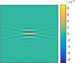
(see Figure 2a for an illustration in the case when θ=0𝜃0\theta=0). In other words, the reconstruction sθsubscript𝑠𝜃s_{\theta} is the result of an integral operator given by the kernel gθsubscript𝑔𝜃g_{\theta} applied to the refractive index n𝑛n. Thus, the next step is the study of the point spread function (PSF) gθ(𝐱,𝐱)subscript𝑔𝜃𝐱superscript𝐱g_{\theta}\left(\mathbf{x},\mathbf{x}^{\prime}\right), which should be thought of as the image corresponding to a delta scatterer in 𝐱superscript𝐱\mathbf{x}^{\prime}.

Refer to caption
(a) The exact PSF given in (6).
Refer to caption
(b) The approximation of the PSF given in (9).
Refer to caption
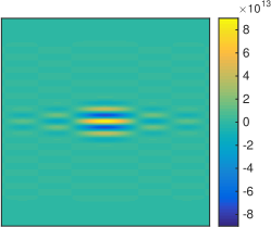
(c) The approximation of the PSF given in (10).
Figure 2: The real part of the point spread function g0subscript𝑔0g_{0} and its approximations are shown in these figures (with parameters as in (1) and (2), and F=0.4𝐹0.4F=0.4). The size of the square shown is 2mm×2mm2mm2mm2\,\mathrm{mm}\times 2\,\mathrm{mm}, and the horizontal and vertical axes are the x𝑥x and z𝑧z axes, respectively. The relative error in the Lsuperscript𝐿L^{\infty} norm is about 7% for the approximation shown in panel (b) and about 9% for the approximation shown in panel (c).

3.2 The point spread function

In its exact form, it does not seem possible to simplify the expression for g𝑔g further: we will have to perform some approximations. First, observe that setting h𝐱,𝐱θ(u)=τ𝐱θ(u)τ𝐱θ(u)superscriptsubscript𝐱superscript𝐱𝜃𝑢superscriptsubscript𝜏𝐱𝜃𝑢superscriptsubscript𝜏superscript𝐱𝜃𝑢h_{\mathbf{x},\mathbf{x}^{\prime}}^{\theta}(u)=\tau_{\mathbf{x}}^{\theta}\left(u\right)-\tau_{\mathbf{x}^{\prime}}^{\theta}\left(u\right) for 𝐱,𝐱+2𝐱superscript𝐱superscriptsubscript2\mathbf{x},\mathbf{x}^{\prime}\in\mathbb{R}_{+}^{2} we readily derive

(h𝐱,𝐱θ)(u)=c01(ux|𝐱𝐮0|ux|𝐱𝐮0|)c01(ux|𝐱𝐮0|ux|𝐱𝐮0|)=c01xx|𝐱𝐮0|,superscriptsuperscriptsubscript𝐱superscript𝐱𝜃𝑢superscriptsubscript𝑐01𝑢𝑥𝐱subscript𝐮0𝑢superscript𝑥superscript𝐱subscript𝐮0superscriptsubscript𝑐01𝑢𝑥superscript𝐱subscript𝐮0𝑢superscript𝑥superscript𝐱subscript𝐮0superscriptsubscript𝑐01superscript𝑥𝑥superscript𝐱subscript𝐮0(h_{\mathbf{x},\mathbf{x}^{\prime}}^{\theta})^{\prime}(u)=c_{0}^{-1}(\frac{u-x}{|\mathbf{x}-{\bf u}_{0}|}-\frac{u-x^{\prime}}{|\mathbf{x}^{\prime}-{\bf u}_{0}|})\approx c_{0}^{-1}(\frac{u-x}{|\mathbf{x}^{\prime}-{\bf u}_{0}|}-\frac{u-x^{\prime}}{|\mathbf{x}^{\prime}-{\bf u}_{0}|})=c_{0}^{-1}\frac{x^{\prime}-x}{|\mathbf{x}^{\prime}-{\bf u}_{0}|},

for 𝐱𝐱\mathbf{x} close to 𝐱superscript𝐱\mathbf{x}^{\prime} (note that, otherwise, the magnitude of the PSF would be substantially lower). As a consequence, by (6) we have

gθ(𝐱,𝐱)c0(4π)1xxxFzx+Fz(h𝐱,𝐱θ)(u)f′′(h𝐱,𝐱θ(u))𝑑u=c0(4π)1xx[f(h𝐱,𝐱θ(x+Fz))f(h𝐱,𝐱θ(xFz))].subscript𝑔𝜃𝐱superscript𝐱subscript𝑐0superscript4𝜋1𝑥superscript𝑥superscriptsubscript𝑥𝐹𝑧𝑥𝐹𝑧superscriptsuperscriptsubscript𝐱superscript𝐱𝜃𝑢superscript𝑓′′superscriptsubscript𝐱superscript𝐱𝜃𝑢differential-d𝑢subscript𝑐0superscript4𝜋1𝑥superscript𝑥delimited-[]superscript𝑓superscriptsubscript𝐱superscript𝐱𝜃𝑥𝐹𝑧superscript𝑓superscriptsubscript𝐱superscript𝐱𝜃𝑥𝐹𝑧\begin{split}g_{\theta}\left(\mathbf{x},\mathbf{x}^{\prime}\right)&\approx\frac{c_{0}(4\pi)^{-1}}{x-x^{\prime}}\int_{x-Fz}^{x+Fz}(h_{\mathbf{x},\mathbf{x}^{\prime}}^{\theta})^{\prime}(u)f^{\prime\prime}\left(h_{\mathbf{x},\mathbf{x}^{\prime}}^{\theta}(u)\right)du\\ &=\frac{c_{0}(4\pi)^{-1}}{x-x^{\prime}}\left[f^{\prime}(h_{\mathbf{x},\mathbf{x}^{\prime}}^{\theta}(x+Fz))-f^{\prime}(h_{\mathbf{x},\mathbf{x}^{\prime}}^{\theta}(x-Fz))\right].\end{split} (7)

In order to simplify this expression even further, let us do a Taylor expansion of w±θ(x,z):=h𝐱,𝐱θ(x±Fz)assignsuperscriptsubscript𝑤plus-or-minus𝜃𝑥𝑧superscriptsubscript𝐱superscript𝐱𝜃plus-or-minus𝑥𝐹𝑧w_{\pm}^{\theta}(x,z):=h_{\mathbf{x},\mathbf{x}^{\prime}}^{\theta}(x\pm Fz) with respect to (x,z)𝑥𝑧(x,z) around (x,z)superscript𝑥superscript𝑧(x^{\prime},z^{\prime}). Direct calculations show that

w±θ(x,z)=0,w±θ(x,z)=c011+F2(1+F2sinθF,1+1+F2cosθ),formulae-sequencesuperscriptsubscript𝑤plus-or-minus𝜃superscript𝑥superscript𝑧0superscriptsubscript𝑤plus-or-minus𝜃superscript𝑥superscript𝑧superscriptsubscript𝑐011superscript𝐹2minus-or-plus1superscript𝐹2𝜃𝐹11superscript𝐹2𝜃w_{\pm}^{\theta}(x^{\prime},z^{\prime})=0,\qquad\nabla w_{\pm}^{\theta}(x^{\prime},z^{\prime})=\frac{c_{0}^{-1}}{\sqrt{1+F^{2}}}(\sqrt{1+F^{2}}\sin\theta\mp F,1+\sqrt{1+F^{2}}\cos\theta),

whence

h𝐱,𝐱θ(x±Fz)c011+F2((1+1+F2cosθ)(zz)+(1+F2sinθF)(xx)).superscriptsubscript𝐱superscript𝐱𝜃plus-or-minus𝑥𝐹𝑧superscriptsubscript𝑐011superscript𝐹211superscript𝐹2𝜃𝑧superscript𝑧minus-or-plus1superscript𝐹2𝜃𝐹𝑥superscript𝑥h_{\mathbf{x},\mathbf{x}^{\prime}}^{\theta}(x\pm Fz)\!\approx\!\frac{c_{0}^{-1}}{\sqrt{1+F^{2}}}\left(\!(1+\sqrt{1+F^{2}}\cos\theta)(z-z^{\prime})\!+\!(\sqrt{1+F^{2}}\sin\theta\mp F)(x-x^{\prime})\!\right)\!.

Substituting this expression into (7) yields

gθ(𝐱,𝐱)g~θ(𝐱𝐱),subscript𝑔𝜃𝐱superscript𝐱subscript~𝑔𝜃𝐱superscript𝐱g_{\theta}(\mathbf{x},\mathbf{x}^{\prime})\approx\tilde{g}_{\theta}(\mathbf{x}-\mathbf{x}^{\prime}), (8)

where

g~θ(𝐱)=c04πx[f(c011+F2((1+1+F2cosθ)z+(1+F2sinθF)x))f(c011+F2((1+1+F2cosθ)z+(1+F2sinθ+F)x))],subscript~𝑔𝜃𝐱subscript𝑐04𝜋𝑥delimited-[]superscript𝑓superscriptsubscript𝑐011superscript𝐹211superscript𝐹2𝜃𝑧1superscript𝐹2𝜃𝐹𝑥superscript𝑓superscriptsubscript𝑐011superscript𝐹211superscript𝐹2𝜃𝑧1superscript𝐹2𝜃𝐹𝑥\tilde{g}_{\theta}(\mathbf{x})=\frac{c_{0}}{4\pi x}\left[f^{\prime}\left(\frac{c_{0}^{-1}}{\sqrt{1+F^{2}}}\left((1+\sqrt{1+F^{2}}\cos\theta)z+(\sqrt{1+F^{2}}\sin\theta-F)x\right)\right)\right.\\ \left.-f^{\prime}\left(\frac{c_{0}^{-1}}{\sqrt{1+F^{2}}}\left((1+\sqrt{1+F^{2}}\cos\theta)z+(\sqrt{1+F^{2}}\sin\theta+F)x\right)\right)\right], (9)

(see Figure 2b for an illustration in the case θ=0𝜃0\theta=0), thereby allowing to write the image sθsubscript𝑠𝜃s_{\theta} given in (5) as a convolution of g~θsubscript~𝑔𝜃\tilde{g}_{\theta} and the refractive index n𝑛n, namely

sθ(𝐱)=𝐱2g~θ(𝐱𝐱)n(𝐱)𝑑𝐱=(g~θn)(𝐱),𝐱+2.formulae-sequencesubscript𝑠𝜃𝐱subscriptsuperscript𝐱superscript2subscript~𝑔𝜃𝐱superscript𝐱𝑛superscript𝐱differential-dsuperscript𝐱subscript~𝑔𝜃𝑛𝐱𝐱superscriptsubscript2s_{\theta}(\mathbf{x})=\int_{\mathbf{x^{\prime}}\in\mathbb{R}^{2}}\tilde{g}_{\theta}(\mathbf{x}-\mathbf{x}^{\prime})n\left(\mathbf{x}^{\prime}\right)d\mathbf{x}^{\prime}=(\tilde{g}_{\theta}*n)(\mathbf{x}),\qquad\mathbf{x}\in\mathbb{R}_{+}^{2}.

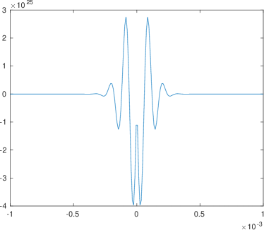
The validity of this approximation, obtained by truncating the Taylor expansion of w±θsuperscriptsubscript𝑤plus-or-minus𝜃w_{\pm}^{\theta} at the first order, is by no means obvious. Indeed, by construction, the pulse f(t)𝑓𝑡f(t) is highly oscillating (ν06106s1subscript𝜈06superscript106superscripts1\nu_{0}\approx 6\cdot 10^{6}\,\mathrm{s^{-1}}), and therefore even small variations in t𝑡t may result in substantial changes in f(t)𝑓𝑡f(t). However, this does not happen, since if (x,z)𝑥𝑧(x,z) is not very close to (x,z)superscript𝑥superscript𝑧(x^{\prime},z^{\prime}) then the magnitude of the PSF is very small, if compared to the maximum value. The verification of this fact is quite technical, and thus is omitted: the details may be found in Appendix A.

Remark 1.

From this expression, it is easy to understand the role of the aperture parameter F𝐹F, which depends on the directivity of the array. Ignoring the second order effect in F𝐹F and taking, for simplicity θ=0𝜃0\theta=0, we can further simplify the above expression as

g~0(𝐱)c04πx[f(c01(2zFx))f(c01(2z+Fx))].subscript~𝑔0𝐱subscript𝑐04𝜋𝑥delimited-[]superscript𝑓superscriptsubscript𝑐012𝑧𝐹𝑥superscript𝑓superscriptsubscript𝑐012𝑧𝐹𝑥\tilde{g}_{0}(\mathbf{x})\approx\frac{c_{0}}{4\pi x}\left[f^{\prime}\left(c_{0}^{-1}\left(2z-Fx\right)\right)-f^{\prime}\left(c_{0}^{-1}\left(2z+Fx\right)\right)\right].

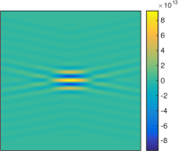
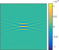
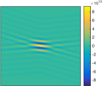
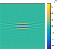
It is clear that F𝐹F affects the resolution in the variable x𝑥x: the higher F𝐹F is, the higher the resolution is. Moreover, the aperture parameter affects also the orientation of the diagonal tails in the PSF. These two phenomena can be clearly seen in Figure 3. In general, the higher the aperture is the better for the reconstruction: as expected, the intrinsic properties of the array affects the reconstruction.

Refer to caption
(a) The PSF with F=0.2𝐹0.2F=0.2.
Refer to caption
(b) The PSF with F=0.3𝐹0.3F=0.3.
Refer to caption
(c) The PSF with F=0.4𝐹0.4F=0.4.
Refer to caption
(d) The PSF with F=0.5𝐹0.5F=0.5.
Figure 3: The exact PSF with different values of the aperture parameter F𝐹F (with parameters as in (1) and (2), and θ=0𝜃0\theta=0). The size of the square shown is 2mm×2mm2mm2mm2\,\mathrm{mm}\times 2\,\mathrm{mm}, and the horizontal and vertical axes are the x𝑥x and z𝑧z axes, respectively.
Remark 2.

It is also easy to understand the role of the angle θ𝜃\theta. In view of

g~θ(𝐱)c04πx[f(c01((1+cosθ)z+(sinθF)x))f(c01((1+cosθ)z+(sinθ+F)x))],subscript~𝑔𝜃𝐱subscript𝑐04𝜋𝑥delimited-[]superscript𝑓superscriptsubscript𝑐011𝜃𝑧𝜃𝐹𝑥superscript𝑓superscriptsubscript𝑐011𝜃𝑧𝜃𝐹𝑥\tilde{g}_{\theta}(\mathbf{x})\approx\frac{c_{0}}{4\pi x}\left[f^{\prime}\left(c_{0}^{-1}\left((1+\cos\theta)z+(\sin\theta-F)x\right)\right)\right.\\ \left.-f^{\prime}\left(c_{0}^{-1}\left((1+\cos\theta)z+(\sin\theta+F)x\right)\right)\right],

an angle θ0𝜃0\theta\neq 0 substantially gives a rotation of the PSF; see Figure 4.

Refer to caption
(a) The PSF with θ=0𝜃0\theta=0.
Refer to caption
(b) The PSF with θ=0.1𝜃0.1\theta=0.1.
Refer to caption
(c) The PSF with θ=0.2𝜃0.2\theta=0.2.
Refer to caption
(d) The PSF with θ=0.3𝜃0.3\theta=0.3.
Figure 4: The exact PSF with different values of the angle θ𝜃\theta (with parameters as in (1) and (2), and F=0.4𝐹0.4F=0.4). The size of the square shown is 2mm×2mm2mm2mm2\,\mathrm{mm}\times 2\,\mathrm{mm}, and the horizontal and vertical axes are the x𝑥x and z𝑧z axes, respectively.

We have now expressed gθsubscript𝑔𝜃g_{\theta} as a convolution kernel. In order to better understand the different roles of the variables x𝑥x and z𝑧z, it is instructive to use the actual expression for f𝑓f given in (1). Since f(t)=ν0e2πiν0tχ~(ν0t)superscript𝑓𝑡subscript𝜈0superscript𝑒2𝜋𝑖subscript𝜈0𝑡~𝜒subscript𝜈0𝑡f^{\prime}(t)=\nu_{0}e^{2\pi i\nu_{0}t}\tilde{\chi}(\nu_{0}t), with χ~(t)=2πiχ(t)+χ(t)~𝜒𝑡2𝜋𝑖𝜒𝑡superscript𝜒𝑡\tilde{\chi}(t)=2\pi i\chi(t)+\chi^{\prime}(t), we can write

f(c011+F2((1+1+F2cosθ)z+(1+F2sinθ±F)x))=ν0e2πiν0c011+F2((1+1+F2cosθ)z+(1+F2sinθ±F)x)χ~(ν0c011+F2((1+1+F2cosθ)z+(1+F2sinθ±F)x))ν0e2πiν0c01(2z+(θ±F)x)χ~(2ν0c01z),superscript𝑓superscriptsubscript𝑐011superscript𝐹211superscript𝐹2𝜃𝑧plus-or-minus1superscript𝐹2𝜃𝐹𝑥subscript𝜈0superscript𝑒2𝜋𝑖subscript𝜈0superscriptsubscript𝑐011superscript𝐹211superscript𝐹2𝜃𝑧plus-or-minus1superscript𝐹2𝜃𝐹𝑥~𝜒subscript𝜈0superscriptsubscript𝑐011superscript𝐹211superscript𝐹2𝜃𝑧plus-or-minus1superscript𝐹2𝜃𝐹𝑥subscript𝜈0superscript𝑒2𝜋𝑖subscript𝜈0superscriptsubscript𝑐012𝑧plus-or-minus𝜃𝐹𝑥~𝜒2subscript𝜈0superscriptsubscript𝑐01𝑧\begin{split}f^{\prime}&\left(\frac{c_{0}^{-1}}{\sqrt{1+F^{2}}}\left((1+\sqrt{1+F^{2}}\cos\theta)z+(\sqrt{1+F^{2}}\sin\theta\pm F)x\right)\right)\\ &=\nu_{0}e^{\frac{2\pi i\nu_{0}c_{0}^{-1}}{\sqrt{1+F^{2}}}\left((1+\sqrt{1+F^{2}}\cos\theta)z+(\sqrt{1+F^{2}}\sin\theta\pm F)x\right)}\\ &\quad\tilde{\chi}\left(\frac{\nu_{0}c_{0}^{-1}}{\sqrt{1+F^{2}}}\left((1+\sqrt{1+F^{2}}\cos\theta)z+(\sqrt{1+F^{2}}\sin\theta\pm F)x\right)\right)\\ &\approx\nu_{0}e^{2\pi i\nu_{0}c_{0}^{-1}\left(2z+(\theta\pm F)x\right)}\tilde{\chi}\left(2\nu_{0}c_{0}^{-1}z\right),\end{split}

where we have approximated the dependence on F𝐹F and θ𝜃\theta at first order around F=0𝐹0F=0 and θ=0𝜃0\theta=0 in the complex exponential (recall that F𝐹F and θ𝜃\theta are small) and at zero-th order (F=0𝐹0F=0 and θ=0𝜃0\theta=0) inside χ~~𝜒\tilde{\chi}: the difference in the orders is motivated by the fact that the variations of the complex exponentials have much higher frequencies than those of χ~~𝜒\tilde{\chi}, since several oscillations are contained in the envelope defined by χ𝜒\chi, as it can be easily seen in Figure 1a (and similarly for χsuperscript𝜒\chi^{\prime}). This approximation may be justified by arguing as in Appendix A. Inserting this expression into (9) yields

g~θ(𝐱)c04πx[ν0e2πiν0c01(2z+(θF)x)χ~(2ν0c01z)ν0e2πiν0c01(2z+(θ+F)x)χ~(2ν0c01z)]=iν0c02πxχ~(2ν0c01z)e4πiν0c01ze2πiν0c01θxsin(2πν0c01Fx),subscript~𝑔𝜃𝐱subscript𝑐04𝜋𝑥delimited-[]subscript𝜈0superscript𝑒2𝜋𝑖subscript𝜈0superscriptsubscript𝑐012𝑧𝜃𝐹𝑥~𝜒2subscript𝜈0superscriptsubscript𝑐01𝑧subscript𝜈0superscript𝑒2𝜋𝑖subscript𝜈0superscriptsubscript𝑐012𝑧𝜃𝐹𝑥~𝜒2subscript𝜈0superscriptsubscript𝑐01𝑧𝑖subscript𝜈0subscript𝑐02𝜋𝑥~𝜒2subscript𝜈0superscriptsubscript𝑐01𝑧superscript𝑒4𝜋𝑖subscript𝜈0superscriptsubscript𝑐01𝑧superscript𝑒2𝜋𝑖subscript𝜈0superscriptsubscript𝑐01𝜃𝑥2𝜋subscript𝜈0superscriptsubscript𝑐01𝐹𝑥\begin{split}\tilde{g}_{\theta}(\mathbf{x})&\approx\frac{c_{0}}{4\pi x}\left[\nu_{0}e^{2\pi i\nu_{0}c_{0}^{-1}\left(2z+(\theta-F)x\right)}\tilde{\chi}\left(2\nu_{0}c_{0}^{-1}z\right)\!-\!\nu_{0}e^{2\pi i\nu_{0}c_{0}^{-1}\left(2z+(\theta+F)x\right)}\tilde{\chi}\left(2\nu_{0}c_{0}^{-1}z\right)\right]\\ &=-\frac{i\nu_{0}c_{0}}{2\pi x}\,\tilde{\chi}\left(2\nu_{0}c_{0}^{-1}z\right)e^{4\pi i\nu_{0}c_{0}^{-1}z}e^{2\pi i\nu_{0}c_{0}^{-1}\theta x}\,\sin(2\pi\nu_{0}c_{0}^{-1}Fx),\end{split}

whence for every 𝐱=(x,z)2𝐱𝑥𝑧superscript2\mathbf{x}=(x,z)\in\mathbb{R}^{2}

g~θ(𝐱)iν02Fχ~(2ν0c01z)e4πiν0c01ze2πiν0c01θxsinc(2πν0c01Fx),subscript~𝑔𝜃𝐱𝑖superscriptsubscript𝜈02𝐹~𝜒2subscript𝜈0superscriptsubscript𝑐01𝑧superscript𝑒4𝜋𝑖subscript𝜈0superscriptsubscript𝑐01𝑧superscript𝑒2𝜋𝑖subscript𝜈0superscriptsubscript𝑐01𝜃𝑥sinc2𝜋subscript𝜈0superscriptsubscript𝑐01𝐹𝑥\tilde{g}_{\theta}(\mathbf{x})\approx-i\nu_{0}^{2}F\tilde{\chi}\left(2\nu_{0}c_{0}^{-1}z\right)e^{4\pi i\nu_{0}c_{0}^{-1}z}e^{2\pi i\nu_{0}c_{0}^{-1}\theta x}\,\mathrm{sinc}(2\pi\nu_{0}c_{0}^{-1}Fx), (10)

where sinc(x):=sin(x)/xassignsinc𝑥𝑥𝑥\mathrm{sinc}(x):=\sin(x)/x (see Figure 2c). This final expression allows us to analyze the PSF g~θsubscript~𝑔𝜃\tilde{g}_{\theta}, and in particular its different behaviors with respect to the variables x𝑥x and z𝑧z. Consider for simplicity the case θ=0𝜃0\theta=0 (with τ=1𝜏1\tau=1). In view of the term χ~(2ν0c01z)~𝜒2subscript𝜈0superscriptsubscript𝑐01𝑧\tilde{\chi}\left(2\nu_{0}c_{0}^{-1}z\right), the vertical resolution is approximately 0.8ν01c00.8superscriptsubscript𝜈01subscript𝑐00.8\cdot\nu_{0}^{-1}c_{0}; similarly, in view of the term sinc(2πν0c01Fx)sinc2𝜋subscript𝜈0superscriptsubscript𝑐01𝐹𝑥\mathrm{sinc}(2\pi\nu_{0}c_{0}^{-1}Fx), the horizontal resolution is approximately 12Fν01c012𝐹superscriptsubscript𝜈01subscript𝑐0\frac{1}{2F}\,\nu_{0}^{-1}c_{0}. Even though horizontal and vertical resolutions are comparable, in terms of focusing and frequencies of oscillations the PSF has very different behaviours in the two directions. Indeed, we can observe that the focusing in the variable z𝑧z is sharper than that in the variable x𝑥x: the decay of χ~~𝜒\tilde{\chi} is much stronger than the decay of sincsinc\mathrm{sinc}. Moreover, in the variable z𝑧z we have only high oscillations, while in the variable x𝑥x the highest oscillations are at least four times slower (2=4124F24124𝐹2=4\frac{1}{2}\geq 4F), and very low frequencies are present as well, due to the presence of the sincsinc\mathrm{sinc}. As it is clear from Figure 2, this approximation introduces evident distortions of the tails, as it is expected from the approximation F=0𝐹0F=0 inside χ~~𝜒\tilde{\chi}; however, the center of the PSF is well approximated. Similar considerations are valid for the case when θ0𝜃0\theta\neq 0: as observed before, this simply gives a rotation.

The same analysis may be carried out by looking at the expression of the PSF in the frequency domain. For simplicity, consider the case θ=0𝜃0\theta=0: the general case simply involves a translation in the frequency domain with respect to x𝑥x. Thanks to the separable form of g~θsubscript~𝑔𝜃\tilde{g}_{\theta} given in (10), the Fourier transform may be directly calculated, and results in the product of the Fourier transform of χ~~𝜒\tilde{\chi} and the Fourier transform of the sincsinc\mathrm{sinc}. More precisely, we readily derive

g~θ(ξx,ξz)=2g~θ(x,z)e2πi(xξx+zξz)dxdziν02Fsinc(2πν0c01Fx)e2πixξx𝑑xχ~(ν0c01z)e2πi(2ν0c01+ξz)z𝑑z.subscript~𝑔𝜃subscript𝜉𝑥subscript𝜉𝑧subscriptsuperscript2subscript~𝑔𝜃𝑥𝑧superscript𝑒2𝜋𝑖𝑥subscript𝜉𝑥𝑧subscript𝜉𝑧𝑑𝑥𝑑𝑧𝑖superscriptsubscript𝜈02𝐹subscriptsinc2𝜋subscript𝜈0superscriptsubscript𝑐01𝐹𝑥superscript𝑒2𝜋𝑖𝑥subscript𝜉𝑥differential-d𝑥subscript~𝜒subscript𝜈0superscriptsubscript𝑐01𝑧superscript𝑒2𝜋𝑖2subscript𝜈0superscriptsubscript𝑐01subscript𝜉𝑧𝑧differential-d𝑧\begin{split}\mathcal{F}\tilde{g}_{\theta}(\xi_{x},&\xi_{z})=\int_{\mathbb{R}^{2}}\tilde{g}_{\theta}(x,z)e^{-2\pi i(x\xi_{x}+z\xi_{z})}\,dxdz\\ &\approx-i\nu_{0}^{2}F\int_{\mathbb{R}}\mathrm{sinc}(2\pi\nu_{0}c_{0}^{-1}Fx)e^{-2\pi ix\xi_{x}}\,dx\int_{\mathbb{R}}\tilde{\chi}\left(\nu_{0}c_{0}^{-1}z\right)e^{-2\pi i(-2\nu_{0}c_{0}^{-1}+\xi_{z})z}\,dz.\end{split}

Thus, since the Fourier transform of the sincsinc\mathrm{sinc} may be easily computed and is a suitable scaled version of the rectangle function, we have

g~θ(ξx,ξz)iν02F12ν0c01F𝟙[F,F](c0ν01ξx)χ~(ν0c01z)e2πi(2ν0c01+ξz)z𝑑z=ic0ν02𝟙[F,F](c0ν01ξx)1ν0c01χ~(2ν0c01+ξzν0c01),subscript~𝑔𝜃subscript𝜉𝑥subscript𝜉𝑧𝑖superscriptsubscript𝜈02𝐹12subscript𝜈0superscriptsubscript𝑐01𝐹subscript1𝐹𝐹subscript𝑐0superscriptsubscript𝜈01subscript𝜉𝑥subscript~𝜒subscript𝜈0superscriptsubscript𝑐01𝑧superscript𝑒2𝜋𝑖2subscript𝜈0superscriptsubscript𝑐01subscript𝜉𝑧𝑧differential-d𝑧𝑖subscript𝑐0subscript𝜈02subscript1𝐹𝐹subscript𝑐0superscriptsubscript𝜈01subscript𝜉𝑥1subscript𝜈0superscriptsubscript𝑐01~𝜒2subscript𝜈0superscriptsubscript𝑐01subscript𝜉𝑧subscript𝜈0superscriptsubscript𝑐01\begin{split}\mathcal{F}\tilde{g}_{\theta}(\xi_{x},\xi_{z})&\approx-i\nu_{0}^{2}F\frac{1}{2\nu_{0}c_{0}^{-1}F}\mathds{1}_{[-F,F]}\left(c_{0}\nu_{0}^{-1}\xi_{x}\right)\int_{\mathbb{R}}\tilde{\chi}\left(\nu_{0}c_{0}^{-1}z\right)e^{-2\pi i(-2\nu_{0}c_{0}^{-1}+\xi_{z})z}\,dz\\ &=-\frac{ic_{0}\nu_{0}}{2}\mathds{1}_{[-F,F]}\left(c_{0}\nu_{0}^{-1}\xi_{x}\right)\frac{1}{\nu_{0}c_{0}^{-1}}\mathcal{F}\tilde{\chi}\left(\frac{-2\nu_{0}c_{0}^{-1}+\xi_{z}}{\nu_{0}c_{0}^{-1}}\right),\end{split}

whence

g~θ(ξx,ξz)ic02 1[F,F](c0ν01ξx)χ~(2+ν01c0ξz)/2.subscript~𝑔𝜃subscript𝜉𝑥subscript𝜉𝑧𝑖superscriptsubscript𝑐02subscript1𝐹𝐹subscript𝑐0superscriptsubscript𝜈01subscript𝜉𝑥~𝜒2superscriptsubscript𝜈01subscript𝑐0subscript𝜉𝑧2\mathcal{F}\tilde{g}_{\theta}(\xi_{x},\xi_{z})\approx-ic_{0}^{2}\,\mathds{1}_{[-F,F]}\left(c_{0}\nu_{0}^{-1}\xi_{x}\right)\mathcal{F}\tilde{\chi}\left(-2+\nu_{0}^{-1}c_{0}\xi_{z}\right)/2. (11)

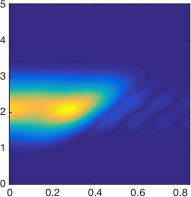
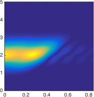
Therefore, up to a constant, the Fourier transform of the PSF is a low-pass filter in the variable x𝑥x with cut-off frequency Fν0c01𝐹subscript𝜈0superscriptsubscript𝑐01F\nu_{0}c_{0}^{-1} and a band pass filter in z𝑧z around 2ν0c012subscript𝜈0superscriptsubscript𝑐012\nu_{0}c_{0}^{-1} (since χ~~𝜒\tilde{\chi} is a low-pass filter). This explains, from another point of view, the different behaviors of g~θsubscript~𝑔𝜃\tilde{g}_{\theta} with respect to x𝑥x and z𝑧z. This difference is evident from Figure 5, where the absolute values of the Fourier transforms of the different approximations of the PSF are shown.
Refer to caption
(a) The Fourier transform of the exact PSF g0subscript𝑔0g_{0} given in (6).
Refer to caption
(b) The Fourier transform of the approximation of the PSF g~0subscript~𝑔0\tilde{g}_{0} given in (9).
Refer to caption
(c) The Fourier transform (11) of the approximation of the PSF g~0subscript~𝑔0\tilde{g}_{0} given in (10).
Refer to caption
(d) The Fourier transform of the PSF gΘacsuperscriptsubscript𝑔Θacg_{\Theta}^{\text{ac}} given in (13), for Θ=0.25Θ0.25\Theta=0.25.
Figure 5: The absolute values of the Fourier transforms of the point spread functions and its approximations (with parameters as in (1) and (2), and F=θ=0𝐹𝜃0F=\theta=0). The frequency axes are normalized by ν0c01subscript𝜈0superscriptsubscript𝑐01\nu_{0}c_{0}^{-1}: the PSF is a low pass filter with cut-off frequency Fν0c01𝐹subscript𝜈0superscriptsubscript𝑐01F\nu_{0}c_{0}^{-1} with respect to the variable x𝑥x and a band pass filter around 2ν0c012subscript𝜈0superscriptsubscript𝑐012\nu_{0}c_{0}^{-1} with respect to z𝑧z.

3.3 Angle compounding

We saw in the previous subsection that, while very focused in the direction z𝑧z, the PSF is not very focused in the direction x𝑥x due to the presence of the sincsinc\mathrm{sinc} function, see (10). In order to have a better focusing, it was proposed in [16] to use multiple measurements corresponding to many angles in an interval θ[Θ,Θ]𝜃ΘΘ\theta\in[-\Theta,\Theta] for some 0Θ0.250Θ0.250\leq\Theta\leq 0.25. The reason why this technique is promising is evident from Figure 4: adding up several angles together will result in an enhancement of the center of the PSF, and in a substantial reduction of the artifacts caused by the tails in the direction x𝑥x. Let us now analyze this phenomenon analytically.

In a continuous setting, angle compounding corresponds to setting

sΘac(𝐱)=12ΘΘΘsθ(𝐱)𝑑θ,𝐱+2.formulae-sequencesuperscriptsubscript𝑠Θac𝐱12ΘsuperscriptsubscriptΘΘsubscript𝑠𝜃𝐱differential-d𝜃𝐱superscriptsubscript2s_{\Theta}^{\text{ac}}(\mathbf{x})=\frac{1}{2\Theta}\int_{-\Theta}^{\Theta}s_{\theta}(\mathbf{x})\,d\theta,\qquad\mathbf{x}\in\mathbb{R}_{+}^{2}. (12)

Thus, by linearity, the corresponding PSF is given by

gΘac(𝐱,𝐱)=12ΘΘΘgθ(𝐱,𝐱)𝑑θ,𝐱,𝐱+2.formulae-sequencesuperscriptsubscript𝑔Θac𝐱superscript𝐱12ΘsuperscriptsubscriptΘΘsubscript𝑔𝜃𝐱superscript𝐱differential-d𝜃𝐱superscript𝐱superscriptsubscript2g_{\Theta}^{\text{ac}}(\mathbf{x},\mathbf{x}^{\prime})=\frac{1}{2\Theta}\int_{-\Theta}^{\Theta}g_{\theta}(\mathbf{x},\mathbf{x}^{\prime})\,d\theta,\qquad\mathbf{x},\mathbf{x}^{\prime}\in\mathbb{R}_{+}^{2}. (13)
Refer to caption
(a) The PSF gθsubscript𝑔𝜃g_{\theta} with θ=0𝜃0\theta=0.
Refer to caption
(b) The PSF gΘacsuperscriptsubscript𝑔Θacg_{\Theta}^{\text{ac}} with Θ=0.25Θ0.25\Theta=0.25.
Refer to caption
(c) The PSF g~Θacsuperscriptsubscript~𝑔Θac\tilde{g}_{\Theta}^{\text{ac}} with Θ=0.25Θ0.25\Theta=0.25.
Figure 6: A comparison of the PSF related to the single illumination with the PSF associated to multiple angles (with parameters as in (1) and (2), and F=0.4𝐹0.4F=0.4). The better focusing in the variable x𝑥x for gΘacsuperscriptsubscript𝑔Θacg_{\Theta}^{\text{ac}} is evident, as well as the good approximation given by g~Θacsuperscriptsubscript~𝑔Θac\tilde{g}_{\Theta}^{\text{ac}}. The size of the square shown is 2mm×2mm2mm2mm2\,\mathrm{mm}\times 2\,\mathrm{mm}, and the horizontal and vertical axes are the x𝑥x and z𝑧z axes, respectively.

Let us find a simple expression for gΘacsuperscriptsubscript𝑔Θacg_{\Theta}^{\text{ac}}. By using (8), we may write gΘac(𝐱,𝐱)g~Θac(𝐱𝐱)superscriptsubscript𝑔Θac𝐱superscript𝐱superscriptsubscript~𝑔Θac𝐱superscript𝐱g_{\Theta}^{\text{ac}}(\mathbf{x},\mathbf{x}^{\prime})\approx\tilde{g}_{\Theta}^{\text{ac}}(\mathbf{x}-\mathbf{x}^{\prime}), where g~Θacsuperscriptsubscript~𝑔Θac\tilde{g}_{\Theta}^{\text{ac}} is given by g~Θac(𝐱)=12ΘΘΘg~θ(𝐱)𝑑θsuperscriptsubscript~𝑔Θac𝐱12ΘsuperscriptsubscriptΘΘsubscript~𝑔𝜃𝐱differential-d𝜃\tilde{g}_{\Theta}^{\text{ac}}(\mathbf{x})=\frac{1}{2\Theta}\int_{-\Theta}^{\Theta}\tilde{g}_{\theta}(\mathbf{x})\,d\theta, so that the image may be expressed as

sΘac(𝐱)=(g~Θacn)(𝐱),𝐱+2.formulae-sequencesuperscriptsubscript𝑠Θac𝐱superscriptsubscript~𝑔Θac𝑛𝐱𝐱superscriptsubscript2s_{\Theta}^{\text{ac}}(\mathbf{x})=(\tilde{g}_{\Theta}^{\text{ac}}*n)(\mathbf{x}),\qquad\mathbf{x}\in\mathbb{R}_{+}^{2}. (14)

Thus, in view of the approximation (10), we can write

g~Θac(𝐱)=iν02F2ΘΘΘχ~(2ν0c01z)e4πiν0c01ze2πiν0c01θxsinc(2πν0c01Fx)𝑑θ=iν02Fχ~(2ν0c01z)e2iν0c01zsinc(2πν0c01Fx)sinc(2πν0c01Θx).superscriptsubscript~𝑔Θac𝐱𝑖superscriptsubscript𝜈02𝐹2ΘsuperscriptsubscriptΘΘ~𝜒2subscript𝜈0superscriptsubscript𝑐01𝑧superscript𝑒4𝜋𝑖subscript𝜈0superscriptsubscript𝑐01𝑧superscript𝑒2𝜋𝑖subscript𝜈0superscriptsubscript𝑐01𝜃𝑥sinc2𝜋subscript𝜈0superscriptsubscript𝑐01𝐹𝑥differential-d𝜃𝑖superscriptsubscript𝜈02𝐹~𝜒2subscript𝜈0superscriptsubscript𝑐01𝑧superscript𝑒2𝑖subscript𝜈0superscriptsubscript𝑐01𝑧sinc2𝜋subscript𝜈0superscriptsubscript𝑐01𝐹𝑥sinc2𝜋subscript𝜈0superscriptsubscript𝑐01Θ𝑥\begin{split}\tilde{g}_{\Theta}^{\text{ac}}(\mathbf{x})&=-\frac{i\nu_{0}^{2}F}{2\Theta}\int_{-\Theta}^{\Theta}\tilde{\chi}\left(2\nu_{0}c_{0}^{-1}z\right)e^{4\pi i\nu_{0}c_{0}^{-1}z}e^{2\pi i\nu_{0}c_{0}^{-1}\theta x}\,\mathrm{sinc}(2\pi\nu_{0}c_{0}^{-1}Fx)\,d\theta\\ &=-i\nu_{0}^{2}F\tilde{\chi}\left(2\nu_{0}c_{0}^{-1}z\right)e^{2i\nu_{0}c_{0}^{-1}z}\mathrm{sinc}(2\pi\nu_{0}c_{0}^{-1}Fx)\mathrm{sinc}(2\pi\nu_{0}c_{0}^{-1}\Theta x).\end{split}

Therefore, we immediately obtain

g~Θac(𝐱)=g~0(𝐱)sinc(2πν0c01Θx),𝐱2.formulae-sequencesuperscriptsubscript~𝑔Θac𝐱subscript~𝑔0𝐱sinc2𝜋subscript𝜈0superscriptsubscript𝑐01Θ𝑥𝐱superscript2\tilde{g}_{\Theta}^{\text{ac}}(\mathbf{x})=\tilde{g}_{0}(\mathbf{x})\mathrm{sinc}(2\pi\nu_{0}c_{0}^{-1}\Theta x),\qquad\mathbf{x}\in\mathbb{R}^{2}. (15)

This expression shows that the PSF related to angle compounding is nothing else than the PSF related to the single angle imaging with θ=0𝜃0\theta=0 multiplied by sinc(2πν0c01Θx)sinc2𝜋subscript𝜈0superscriptsubscript𝑐01Θ𝑥\mathrm{sinc}(2\pi\nu_{0}c_{0}^{-1}\Theta x). Thus, for Θ=0Θ0\Theta=0 we recover g~θsubscript~𝑔𝜃\tilde{g}_{\theta} for θ=0𝜃0\theta=0, as expected. However, for Θ>0Θ0\Theta>0, this PSF enjoys faster decay in the variable x𝑥x. See Figure 6 for an illustration of gΘacsuperscriptsubscript𝑔Θacg_{\Theta}^{\text{ac}} and g~Θacsuperscriptsubscript~𝑔Θac\tilde{g}_{\Theta}^{\text{ac}} and a comparison with gθsubscript𝑔𝜃g_{\theta} and Figure 5d for an illustration of the Fourier transform of gΘacsuperscriptsubscript𝑔Θacg_{\Theta}^{\text{ac}}.

To sum up the main features of the static problem, we have shown that the recovered image may be written as sΘac=g~Θacnsuperscriptsubscript𝑠Θacsuperscriptsubscript~𝑔Θac𝑛s_{\Theta}^{\text{ac}}=\tilde{g}_{\Theta}^{\text{ac}}*n, where g~Θacsuperscriptsubscript~𝑔Θac\tilde{g}_{\Theta}^{\text{ac}} is the PSF of the imaging system with measurements taken at multiple angles. The ultrafast imaging technique is based on obtaining many of these images over time, as we discuss in the next section.

4 The Dynamic Forward Problem

4.1 The quasi-static approximation and the construction of the data

The dynamic imaging setup consists in the repetition of the static imaging method over time to acquire a collection of images of a medium in motion. We consider a quasi-static model: the whole process of obtaining one image, using the image compounding technique discussed in Subsection 3.3, is fast enough to consider the medium static, but collecting several images over time gives us a movie of the movement over time. In other words, there are two time scales: the fast one related to the propagation of the wave is considered instantaneous with respect to the slow one, related to the sequence of the images.

In view of this quasi-static approximation, from now on we neglect the time of the propagation of a single wave to obtain static imaging. The time t𝑡t considered here is related to the slow time scale. In other words, by (14) at fixed time t𝑡t we obtain a static image s(𝐱,t)𝑠𝐱𝑡s(\mathbf{x},t) of the medium n=n(𝐱,t)𝑛𝑛𝐱𝑡n=n(\mathbf{x},t), namely

s(𝐱,t)=(g~Θacn(,t))(𝐱).𝑠𝐱𝑡superscriptsubscript~𝑔Θac𝑛𝑡𝐱s(\mathbf{x},t)=\left(\tilde{g}_{\Theta}^{\text{ac}}*n(\,\cdot\,,t)\right)(\mathbf{x}). (16)

Repeating the process for t[0,T]𝑡0𝑇t\in[0,T] we obtain the movie s(𝐱,t)𝑠𝐱𝑡s(\mathbf{x},t), which represents the main data we now need to process. As mentioned in the introduction, our aim is locating the blood vessels within the imaged area, by using the fact that s(𝐱,t)𝑠𝐱𝑡s(\mathbf{x},t) will be strongly influenced by movements in n𝑛n.

4.2 The doppler effect

Measuring the medium speed is an available criterion to separate different sources; thus, we want to see the influence on the image of a single particle in movement, as by linearity the obtained conclusions naturally extend to a group of particles. For a single particle, we are interested in observing the generated Doppler effect in the reconstructed image, namely peaks in the Fourier transform away from zero.

Intuitively, Figure 5d shows that there is a clear difference in the movements depending on their orientation. We want to explore this difference in a more precise way. Let us consider n(x,z,t)=δ(0,vt)(x,z)𝑛𝑥𝑧𝑡subscript𝛿0𝑣𝑡𝑥𝑧n(x,z,t)=\delta_{(0,vt)}(x,z), i.e. a single particle moving in the z𝑧z direction with velocity v𝑣v. The resulting image, as a function of time, is obtained via equations (15) and (16)

s(x,z,t)2g~Θac(xx,zz)δ(0,vt)(x,z)𝑑x𝑑z=g~Θac(x,zvt)=g~0(x,zvt)sinc(2πν0c01Θx).𝑠𝑥𝑧𝑡subscriptsuperscript2superscriptsubscript~𝑔Θac𝑥superscript𝑥𝑧superscript𝑧subscript𝛿0𝑣𝑡superscript𝑥superscript𝑧differential-dsuperscript𝑥differential-dsuperscript𝑧superscriptsubscript~𝑔Θac𝑥𝑧𝑣𝑡subscript~𝑔0𝑥𝑧𝑣𝑡sinc2𝜋subscript𝜈0superscriptsubscript𝑐01Θ𝑥\begin{split}s(x,z,t)&\approx\int_{\mathbb{R}^{2}}\tilde{g}_{\Theta}^{\text{ac}}(x-x^{\prime},z-z^{\prime})\delta_{(0,vt)}(x^{\prime},z^{\prime})dx^{\prime}dz^{\prime}\\ &=\tilde{g}_{\Theta}^{\text{ac}}(x,z-vt)\\ &=\tilde{g}_{0}(x,z-vt)\mathrm{sinc}(2\pi\nu_{0}c_{0}^{-1}\Theta x).\end{split}

Therefore, arguing as in (11), we obtain that the Fourier transform with respect to the time variable t𝑡t of the image is given by

t(s)(x,z,ξ)g~0(x,zvt)e2πiξt𝑑tsinc(2πν0c01Θx)=1ve2πiξzv2(g~0)(x,ξv)sinc(2πν0c01Θx),subscript𝑡𝑠𝑥𝑧𝜉subscriptsubscript~𝑔0𝑥𝑧𝑣𝑡superscript𝑒2𝜋𝑖𝜉𝑡differential-d𝑡sinc2𝜋subscript𝜈0superscriptsubscript𝑐01Θ𝑥1𝑣superscript𝑒2𝜋𝑖𝜉𝑧𝑣subscript2subscript~𝑔0𝑥𝜉𝑣sinc2𝜋subscript𝜈0superscriptsubscript𝑐01Θ𝑥\begin{split}\mathcal{F}_{t}(s)(x,z,\xi)&\approx\int_{\mathbb{R}}\tilde{g}_{0}(x,z-vt)e^{-2\pi i\xi t}dt\ \mathrm{sinc}(2\pi\nu_{0}c_{0}^{-1}\Theta x)\\ &=\frac{1}{v}e^{-2\pi i\frac{\xi z}{v}}\mathcal{F}_{2}(\tilde{g}_{0})(x,-\frac{\xi}{v})\mathrm{sinc}(2\pi\nu_{0}c_{0}^{-1}\Theta x),\end{split}

where 2subscript2\mathcal{F}_{2} is the Fourier transform with respect to the variable z𝑧z. Adopting approximation (10), we obtain

t(s)(x,z,ξ)1viν02Fe2πiξzvsinc(2πν0c01Θx)sinc(2πν0c01Fx)(χ~)(ξ2ν0c01v1).subscript𝑡𝑠𝑥𝑧𝜉1𝑣𝑖superscriptsubscript𝜈02𝐹superscript𝑒2𝜋𝑖𝜉𝑧𝑣sinc2𝜋subscript𝜈0superscriptsubscript𝑐01Θ𝑥sinc2𝜋subscript𝜈0superscriptsubscript𝑐01𝐹𝑥~𝜒𝜉2subscript𝜈0superscriptsubscript𝑐01𝑣1\mathcal{F}_{t}(s)(x,z,\xi)\!\approx\!-\frac{1}{v}i\nu_{0}^{2}Fe^{-2\pi i\frac{\xi z}{v}}\mathrm{sinc}(2\pi\nu_{0}c_{0}^{-1}\Theta x)\mathrm{sinc}(2\pi\nu_{0}c_{0}^{-1}Fx)\mathcal{F}(\tilde{\chi})\Bigl{(}\frac{-\xi}{2\nu_{0}c_{0}^{-1}v}-1\Bigr{)}.

Given the shape of χ~~𝜒\tilde{\chi}, its Fourier transform has a maximum around 0, thus we can see a peak of |t(s)(x,z,ξ)|subscript𝑡𝑠𝑥𝑧𝜉|\mathcal{F}_{t}(s)(x,z,\xi)| when ξ𝜉\xi is around 2ν0c01v2subscript𝜈0superscriptsubscript𝑐01𝑣-2\nu_{0}c_{0}^{-1}v, and so we have the Doppler effect.

In the case when the particle is moving parallel to the detector array, namely n(x,z,t)=δ(vt,0)(x,z)𝑛𝑥𝑧𝑡subscript𝛿𝑣𝑡0𝑥𝑧n(x,z,t)=\delta_{(vt,0)}(x,z), following an analogous procedure as before, we obtain

s(x,z,t)g~0(xvt,z)sinc(2πν0c01Θ(xvt)),𝑠𝑥𝑧𝑡subscript~𝑔0𝑥𝑣𝑡𝑧sinc2𝜋subscript𝜈0superscriptsubscript𝑐01Θ𝑥𝑣𝑡s(x,z,t)\approx\tilde{g}_{0}(x-vt,z)\mathrm{sinc}(2\pi\nu_{0}c_{0}^{-1}\Theta(x-vt)),

and applying the Fourier transform in time yields

t(s)(x,z,ξ)1ve2πiξxv(g~0(,z)sinc(2πν0c01Θ))(ξv).\mathcal{F}_{t}(s)(x,z,\xi)\approx\frac{1}{v}e^{-2\pi i\frac{\xi x}{v}}\mathcal{F}(\tilde{g}_{0}(\cdot,z)\mathrm{sinc}(2\pi\nu_{0}c_{0}^{-1}\Theta\cdot))(-\frac{\xi}{v}).

Using approximation (10), the convolution formula for the Fourier transform and the known transform of the sincsinc\mathrm{sinc} function, gives

t(s)(x,z,ξ)ie2πiξxv4Θvν0c0χ~(2ν0c01z)e4πiν0c01z(𝟙[F,F]𝟙[Θ,Θ])(ξvν0c01).subscript𝑡𝑠𝑥𝑧𝜉𝑖superscript𝑒2𝜋𝑖𝜉𝑥𝑣4Θ𝑣subscript𝜈0subscript𝑐0~𝜒2subscript𝜈0superscriptsubscript𝑐01𝑧superscript𝑒4𝜋𝑖subscript𝜈0superscriptsubscript𝑐01𝑧subscript1𝐹𝐹subscript1ΘΘ𝜉𝑣subscript𝜈0superscriptsubscript𝑐01\mathcal{F}_{t}(s)(x,z,\xi)\approx-i\frac{e^{-2\pi i\frac{\xi x}{v}}}{4\Theta v}\nu_{0}c_{0}\tilde{\chi}(2\nu_{0}c_{0}^{-1}z)e^{4\pi i\nu_{0}c_{0}^{-1}z}(\mathds{1}_{[-F,F]}*\mathds{1}_{[-\Theta,\Theta]})\left(-\frac{\xi}{v\nu_{0}c_{0}^{-1}}\right).

The convolution of these characteristic functions evaluated at η𝜂\eta is equal to the length of interval [F+η,F+η][Θ,Θ]𝐹𝜂𝐹𝜂ΘΘ[-F+\eta,F+\eta]\cap[-\Theta,\Theta], because

(𝟙[F,F]𝟙[Θ,Θ])(η)=𝟙[F,F](ηs)𝟙[Θ,Θ](s)𝑑s=𝟙[F+η,F+η](s)𝟙[Θ,Θ](s)𝑑s.subscript1𝐹𝐹subscript1ΘΘ𝜂subscriptsubscript1𝐹𝐹𝜂𝑠subscript1ΘΘ𝑠differential-d𝑠subscriptsubscript1𝐹𝜂𝐹𝜂𝑠subscript1ΘΘ𝑠differential-d𝑠(\mathds{1}_{[-F,F]}*\mathds{1}_{[-\Theta,\Theta]})(\eta)\!=\!\int_{\mathbb{R}}\mathds{1}_{[-F,F]}(\eta-s)\mathds{1}_{[-\Theta,\Theta]}(s)ds\!=\!\int_{\mathbb{R}}\mathds{1}_{[-F+\eta,F+\eta]}(s)\mathds{1}_{[-\Theta,\Theta]}(s)ds.

Since both intervals are centered at 00, this value is maximized for η𝜂\eta (and thus ξ𝜉\xi) around 00, like in the static case, and so the observed Doppler effect is very small.

These differences are fundamental to understand the capabilities of the method for blood flow imaging. This phenomenon will be experimentally verified in Section 6.

4.3 Multiple scatterer random model

We have seen the effect on the image s(x,z,t)𝑠𝑥𝑧𝑡s(x,z,t) of a single moving particle. We now consider the more realistic case of a medium (either blood vessels or tissue) with a large number of particles in motion. This will allow to study the statistical properties of the resulting measurements.

We consider a rectangular domain Ω=(Lx/2,Lx/2)×(0,Lz)Ωsubscript𝐿𝑥2subscript𝐿𝑥20subscript𝐿𝑧\Omega=(-L_{x}/2,L_{x}/2)\times(0,L_{z}), which consists in N𝑁N point particles. Let us denote the location of particle k𝑘k at time t𝑡t by ak(t)subscript𝑎𝑘𝑡a_{k}(t). In the most general case, each particle is subject to a dynamics

ak(t)=φk(uk,t),ak(0)=uk,formulae-sequencesubscript𝑎𝑘𝑡subscript𝜑𝑘subscript𝑢𝑘𝑡subscript𝑎𝑘0subscript𝑢𝑘a_{k}(t)=\varphi_{k}\left(u_{k},t\right),\qquad a_{k}(0)=u_{k}, (17)

where (uk)k=1,,Nsubscriptsubscript𝑢𝑘𝑘1𝑁\left(u_{k}\right)_{k=1,...,N} are independent uniform random variables on ΩΩ\Omega and (φk)k=1,,Nsubscriptsubscript𝜑𝑘𝑘1𝑁\left(\varphi_{k}\right)_{k=1,...,N} are independent and identically distributed stochastic flows: for instance, they can be the flows of a stochastic differential equation or the deterministic flows of a partial differential equation. Thus, the aksubscript𝑎𝑘a_{k}s are independent and identically distributed stochastic processes. In view of these considerations, we consider the medium given by

n(𝐱,t)=CNk=1Nδak(t)(𝐱),𝑛𝐱𝑡𝐶𝑁superscriptsubscript𝑘1𝑁subscript𝛿subscript𝑎𝑘𝑡𝐱n\left(\mathbf{x},t\right)=\frac{C}{\sqrt{N}}\sum_{k=1}^{N}\delta_{a_{k}\left(t\right)}\left(\mathbf{x}\right), (18)

where C>0𝐶0C>0 denotes the scattering intensity and 1N1𝑁\frac{1}{\sqrt{N}} is the natural normalization factor in view of the central limit theorem.

To avoid minor issues from boundary effects, which are of no interest to us in the analysis of this problem, we assume the periodicity of the medium. In other words, we consider the periodization

np(𝐱,t)=𝐥2n(𝐱+𝐥𝐋,t),subscript𝑛𝑝𝐱𝑡subscript𝐥superscript2𝑛𝐱𝐥𝐋𝑡n_{p}(\mathbf{x},t)=\sum_{\mathbf{l}\in\mathbb{Z}^{2}}n(\mathbf{x}+\mathbf{l}\cdot\mathbf{L},t), (19)

where 𝐋=(Lx,Lz)𝐋subscript𝐿𝑥subscript𝐿𝑧\mathbf{L}=(L_{x},L_{z}). Let g(𝐱):=𝐥2g~Θac(𝐱+𝐥𝐋)assign𝑔𝐱subscript𝐥superscript2superscriptsubscript~𝑔Θac𝐱𝐥𝐋g\left(\mathbf{x}\right):=\sum_{\mathbf{l}\in\mathbb{Z}^{2}}\tilde{g}_{\Theta}^{\text{ac}}\left(\mathbf{x}+\mathbf{l}\cdot\mathbf{L}\right) be the periodic PSF, which is more convenient than g~Θacsuperscriptsubscript~𝑔Θac\tilde{g}_{\Theta}^{\text{ac}} (given by (15)) for a ΩΩ\Omega-periodic medium. The dynamic image s𝑠s is then given by

s(𝐱,t)=(g~Θacnp(,t))(𝐱)=(gn(,t))(𝐱)=CNk=1Ng(𝐱ak(t)).𝑠𝐱𝑡superscriptsubscript~𝑔Θacsubscript𝑛𝑝𝑡𝐱𝑔𝑛𝑡𝐱𝐶𝑁superscriptsubscript𝑘1𝑁𝑔𝐱subscript𝑎𝑘𝑡s(\mathbf{x},t)=(\tilde{g}_{\Theta}^{\text{ac}}*n_{p}\left(\cdot,t\right))\left(\mathbf{x}\right)=(g*n(\,\cdot\,,t))(\mathbf{x})=\frac{C}{\sqrt{N}}\sum_{k=1}^{N}g\left(\mathbf{x}-a_{k}\left(t\right)\right).

Let us also assume for the sake of simplicity that, at every time t𝑡t, ak(t)subscript𝑎𝑘𝑡a_{k}\left(t\right) modulo ΩΩ\Omega is a uniform random variable on ΩΩ\Omega, namely

𝔼𝐥2w(ak(t)+𝐥𝐋)=|Ω|12w(𝐲)𝑑𝐲,wL1(2).formulae-sequence𝔼subscript𝐥superscript2𝑤subscript𝑎𝑘𝑡𝐥𝐋superscriptΩ1subscriptsuperscript2𝑤𝐲differential-d𝐲𝑤superscript𝐿1superscript2\mathbb{E}\sum_{\mathbf{l}\in\mathbb{Z}^{2}}w(a_{k}(t)+\mathbf{l}\cdot\mathbf{L})=|\Omega|^{-1}\int_{\mathbb{R}^{2}}w(\mathbf{y})\,d\mathbf{y},\qquad w\in L^{1}(\mathbb{R}^{2}). (20)

As a simple but quite general example, it is worth noting that in the case when ak(t)=uk+F(t)subscript𝑎𝑘𝑡subscript𝑢𝑘𝐹𝑡a_{k}(t)=u_{k}+F(t), where F(t)𝐹𝑡F(t) is any random process independent of uksubscript𝑢𝑘u_{k}, the above equality is satisfied, since

𝔼𝐥2w(uk+F(t)+𝐥𝐋)=|Ω|1𝔼𝐥2Ωw(𝐲+F(t)+𝐥𝐋)𝑑𝐲=|Ω|12w(𝐲)𝑑𝐲,𝔼subscript𝐥superscript2𝑤subscript𝑢𝑘𝐹𝑡𝐥𝐋superscriptΩ1𝔼subscript𝐥superscript2subscriptΩ𝑤𝐲𝐹𝑡𝐥𝐋differential-d𝐲superscriptΩ1subscriptsuperscript2𝑤𝐲differential-d𝐲\mathbb{E}\sum_{\mathbf{l}\in\mathbb{Z}^{2}}w(u_{k}+F(t)+\mathbf{l}\cdot\mathbf{L})=|\Omega|^{-1}\mathbb{E}\sum_{\mathbf{l}\in\mathbb{Z}^{2}}\int_{\Omega}w(\mathbf{y}+F(t)+\mathbf{l}\cdot\mathbf{L})d\mathbf{y}=|\Omega|^{-1}\int_{\mathbb{R}^{2}}w(\mathbf{y})\,d\mathbf{y},

where the expectation in the first term is taken with respect to uksubscript𝑢𝑘u_{k} and F(t)𝐹𝑡F(t), while in the second term only with respect to F(t)𝐹𝑡F(t).

We now wish to compute the expectation of the random variables present in the expression for s(𝐱,t)𝑠𝐱𝑡s(\mathbf{x},t). By (10) and (15), since g~Θacsuperscriptsubscript~𝑔Θac\tilde{g}_{\Theta}^{\text{ac}} is a derivative of a Schwartz function in the variable z𝑧z, we have 2g~Θac(𝐲)𝑑𝐲=0subscriptsuperscript2superscriptsubscript~𝑔Θac𝐲differential-d𝐲0\int_{\mathbb{R}^{2}}\tilde{g}_{\Theta}^{\text{ac}}(\mathbf{y})d\mathbf{y}=0. Thus, by (20) the expected value may be easily computed as

𝔼(g(𝐱ak(t)))=𝔼𝐥2g~Θac(𝐱ak(t)+𝐥𝐋)=|Ω|12g~Θac(𝐲)𝑑𝐲=0.𝔼𝑔𝐱subscript𝑎𝑘𝑡𝔼subscript𝐥superscript2superscriptsubscript~𝑔Θac𝐱subscript𝑎𝑘𝑡𝐥𝐋superscriptΩ1subscriptsuperscript2superscriptsubscript~𝑔Θac𝐲differential-d𝐲0\mathbb{E}\left(g\left(\mathbf{x}-a_{k}\left(t\right)\right)\right)=\mathbb{E}\sum_{\mathbf{l}\in\mathbb{Z}^{2}}\tilde{g}_{\Theta}^{\text{ac}}(\mathbf{x}-a_{k}(t)+\mathbf{l}\cdot\mathbf{L})=|\Omega|^{-1}\int_{\mathbb{R}^{2}}\tilde{g}_{\Theta}^{\text{ac}}(\mathbf{y})d\mathbf{y}=0. (21)

Let (𝐱i)i=1,,m𝐱subscriptsubscript𝐱𝑖𝑖1subscript𝑚𝐱\left(\mathbf{x}_{i}\right)_{i=1,...,m_{\mathbf{x}}} and (tj)j=1,,mtsubscriptsubscript𝑡𝑗𝑗1subscript𝑚𝑡\left(t_{j}\right)_{j=1,...,m_{t}} be the sampling locations and times respectively. The data may be collected in the Casorati matrix SNm𝐱×mtsubscript𝑆𝑁superscriptsubscript𝑚𝐱subscript𝑚𝑡S_{N}\in\mathbb{C}^{m_{\mathbf{x}}\times m_{t}} defined by

SN(i,j)=s(𝐱i,tj).subscript𝑆𝑁𝑖𝑗𝑠subscript𝐱𝑖subscript𝑡𝑗S_{N}(i,j)=s(\mathbf{x}_{i},t_{j}).

By (21), according to the multivariate central limit theorem, the matrix SNsubscript𝑆𝑁S_{N} converges in distribution to a Gaussian complex matrix Sm𝐱×mt𝑆superscriptsubscript𝑚𝐱subscript𝑚𝑡S\in\mathbb{C}^{m_{\mathbf{x}}\times m_{t}} , the distribution of which is entirely determined by the following correlations, for i,i=1,,m𝐱formulae-sequence𝑖superscript𝑖1subscript𝑚𝐱i,i^{\prime}=1,\dots,m_{\mathbf{x}} and j,j=1,,mtformulae-sequence𝑗superscript𝑗1subscript𝑚𝑡j,j^{\prime}=1,\dots,m_{t}

𝔼(S(i,j))=0,𝔼𝑆𝑖𝑗0\displaystyle\mathbb{E}(S(i,j))=0,
Cov(S(i,j),S(i,j))=C2𝔼(g(𝐱ia1(tj))g(𝐱ia1(tj))),Cov𝑆𝑖𝑗𝑆superscript𝑖superscript𝑗superscript𝐶2𝔼𝑔subscript𝐱𝑖subscript𝑎1subscript𝑡𝑗𝑔subscript𝐱superscript𝑖subscript𝑎1subscript𝑡superscript𝑗\displaystyle\textrm{Cov}\left(S(i,j),S(i^{\prime},j^{\prime})\right)=C^{2}\mathbb{E}\left(g\left(\mathbf{x}_{i}-a_{1}\left(t_{j}\right)\right)g\left(\mathbf{x}_{i^{\prime}}-a_{1}\left(t_{j^{\prime}}\right)\right)\right), (22)
Cov(S(i,j),S(i,j)¯)=C2𝔼(g(𝐱ia1(tj))g(𝐱ia1(tj))¯).Cov𝑆𝑖𝑗¯𝑆superscript𝑖superscript𝑗superscript𝐶2𝔼𝑔subscript𝐱𝑖subscript𝑎1subscript𝑡𝑗¯𝑔subscript𝐱superscript𝑖subscript𝑎1subscript𝑡superscript𝑗\displaystyle\textrm{Cov}\left(S(i,j),\overline{S(i^{\prime},j^{\prime})}\right)=C^{2}\mathbb{E}\left(g\left(\mathbf{x}_{i}-a_{1}\left(t_{j}\right)\right)\overline{g\left(\mathbf{x}_{i^{\prime}}-a_{1}\left(t_{j^{\prime}}\right)\right)}\right). (23)

More precisely, let wm𝐱mt𝑤superscriptsubscript𝑚𝐱subscript𝑚𝑡w\in\mathbb{C}^{m_{\mathbf{x}}m_{t}} be a column vector containing all the entries of S𝑆S. Let v2m𝐱mt𝑣superscript2subscript𝑚𝐱subscript𝑚𝑡v\in\mathbb{C}^{2m_{\mathbf{x}}m_{t}} and V2m𝐱mt×2m𝐱mt𝑉superscript2subscript𝑚𝐱subscript𝑚𝑡2subscript𝑚𝐱subscript𝑚𝑡V\in\mathbb{C}^{2m_{\mathbf{x}}m_{t}\times 2m_{\mathbf{x}}m_{t}} be defined by

v=(w1,w1¯,w2,w2¯,,wm𝐱mt,wm𝐱mt¯)TandV=𝔼(vv¯T).formulae-sequence𝑣superscriptsubscript𝑤1¯subscript𝑤1subscript𝑤2¯subscript𝑤2subscript𝑤subscript𝑚𝐱subscript𝑚𝑡¯subscript𝑤subscript𝑚𝐱subscript𝑚𝑡𝑇and𝑉𝔼𝑣superscript¯𝑣𝑇v=\left(w_{1},\overline{w_{1}},w_{2},\overline{w_{2}},...,w_{m_{\mathbf{x}}m_{t}},\overline{w_{m_{\mathbf{x}}m_{t}}}\right)^{T}\quad\text{and}\quad V=\mathbb{E}\left(v\overline{v}^{T}\right).

The covariance matrix V𝑉V can be easily computed from (22) and (23). Then the probability density function f𝑓f of v𝑣v can be expressed as [4]:

f(v)=1πm𝐱mtdet(V)12exp(12vV1v).𝑓𝑣1superscript𝜋subscript𝑚𝐱subscript𝑚𝑡superscript𝑉1212superscript𝑣superscript𝑉1𝑣f\left(v\right)=\frac{1}{\pi^{m_{\mathbf{x}}m_{t}}\det\left(V\right)^{\frac{1}{2}}}\exp\left(-\frac{1}{2}v^{*}V^{-1}v\right).

Moreover, it is possible to generate samples from this distribution: if X𝑋X is a complex unit variance independent normal random vector, and if V𝑉\sqrt{V} is a square root of V𝑉V, then VX𝑉𝑋\sqrt{V}X is distributed like v𝑣v. This allows for simulations of sample image sequences for a large number of particles with a complexity independent of the number of particles.

The analysis carried out here will allow us to study the distribution of the singular value of the matrix S𝑆S, depending on the properties of the flows φksubscript𝜑𝑘\varphi_{k}. This will be the key ingredient to justify the correct separation of blood and clutter signals by means of the singular value decomposition of the measurements.

5 The Dynamic Inverse Problem: Source Separation

5.1 Formulation of the dynamic inverse problem

As explained in the introduction, the aim of the dynamic inverse problem is blood flow imaging. In other words, we are interested in locating blood vessels, possibly very small, within the medium. The main issue is that the signal s(𝐱,t)𝑠𝐱𝑡s(\mathbf{x},t) is highly corrupted by clutter signal, namely the signal scattered from tissues. In the linearized regime we consider, we may write the refractive index n𝑛n as the sum of a clutter component ncsubscript𝑛𝑐n_{c} and a blood component nbsubscript𝑛𝑏n_{b}, namely n=nc+nb𝑛subscript𝑛𝑐subscript𝑛𝑏n=n_{c}+n_{b}. Blood is located only in small vessels in the medium, whereas clutter signal comes from everywhere: by (3), since blood vessels are smaller than the focusing height, even pixels located in blood vessels contain reflections coming from the tissue. Let us denote the location of blood vessels by ΩbΩsubscriptΩ𝑏Ω\Omega_{b}\subset\Omega. The inverse problem is the following: can we recover ΩbsubscriptΩ𝑏\Omega_{b} from the data s(𝐱,t)=sc(𝐱,t)+sb(𝐱,t)𝑠𝐱𝑡subscript𝑠𝑐𝐱𝑡subscript𝑠𝑏𝐱𝑡s(\mathbf{x},t)=s_{c}(\mathbf{x},t)+s_{b}(\mathbf{x},t)? Here, scsubscript𝑠𝑐s_{c} and sbsubscript𝑠𝑏s_{b} are given by (16), with n𝑛n replaced by ncsubscript𝑛𝑐n_{c} and nbsubscript𝑛𝑏n_{b}, respectively. In this section, we provide a quantitative analysis of the method described in [8] based on the singular value decomposition (SVD) of s𝑠s.

5.2 The SVD algorithm

We now review the SVD algorithm presented in [8]. The Casorati matrix Sm𝐱×mt𝑆superscriptsubscript𝑚𝐱subscript𝑚𝑡S\in\mathbb{C}^{m_{\mathbf{x}}\times m_{t}} is defined as in previous section by

S(i,j)=s(𝐱i,tj),i{1,,m𝐱},j{1,,mt}.formulae-sequence𝑆𝑖𝑗𝑠subscript𝐱𝑖subscript𝑡𝑗formulae-sequence𝑖1subscript𝑚𝐱𝑗1subscript𝑚𝑡S(i,j)=s\left(\mathbf{x}_{i},t_{j}\right),\qquad i\in\left\{1,...,m_{\mathbf{x}}\right\},\;j\in\left\{1,...,m_{t}\right\}.

Without loss of generality, we further assume that mtm𝐱subscript𝑚𝑡subscript𝑚𝐱m_{t}\leq m_{\mathbf{x}}. We remind the reader that the SVD of S𝑆S is given by

S=k=1mtσkukvk¯T,𝑆superscriptsubscript𝑘1subscript𝑚𝑡subscript𝜎𝑘subscript𝑢𝑘superscript¯subscript𝑣𝑘𝑇S=\sum_{k=1}^{m_{t}}\sigma_{k}u_{k}\overline{v_{k}}^{T},

where (u1,,um𝐱)subscript𝑢1subscript𝑢subscript𝑚𝐱\left(u_{1},...,u_{m_{\mathbf{x}}}\right) and (v1,,vmt)subscript𝑣1subscript𝑣subscript𝑚𝑡\left(v_{1},...,v_{m_{t}}\right) are orthonormal bases of mxsuperscriptsubscript𝑚𝑥\mathbb{C}^{m_{x}} and mtsuperscriptsubscript𝑚𝑡\mathbb{C}^{m_{t}}, and σ1σ2σmt0subscript𝜎1subscript𝜎2subscript𝜎subscript𝑚𝑡0\sigma_{1}\geq\sigma_{2}\geq...\geq\sigma_{m_{t}}\geq 0. For any K1𝐾1K\geq 1, SK=k=1Kσkukvk¯Tsubscript𝑆𝐾superscriptsubscript𝑘1𝐾subscript𝜎𝑘subscript𝑢𝑘superscript¯subscript𝑣𝑘𝑇S_{K}=\sum_{k=1}^{K}\sigma_{k}u_{k}\overline{v_{k}}^{T} is the best rank K𝐾K approximation of S𝑆S in the Frobenius norm. The SVD is a well-known tool for denoising sequences of images, see for example [11]. The idea is that since singular values for the clutter signal are quickly decaying after a certain threshold, the best rank K𝐾K approximation of S𝑆S will contain most of the signal coming from the clutter, provided that K𝐾K is large enough. This could be used to recover clutter data, by applying a “denoising” algorithm, and keeping only SKsubscript𝑆𝐾S_{K}. But it can also be used to recover the blood location, by considering the “power doppler”

S^b,K(i):=k=K+1mtσk2|uk|2(i)=j=1mt|(SSK)(i,j)|2,i{1,,m𝐱}.formulae-sequenceassignsubscript^𝑆𝑏𝐾𝑖superscriptsubscript𝑘𝐾1subscript𝑚𝑡superscriptsubscript𝜎𝑘2superscriptsubscript𝑢𝑘2𝑖superscriptsubscript𝑗1subscript𝑚𝑡superscript𝑆subscript𝑆𝐾𝑖𝑗2𝑖1subscript𝑚𝐱\hat{S}_{b,K}\left(i\right):=\sum_{k=K+1}^{m_{t}}\sigma_{k}^{2}|u_{k}|^{2}(i)=\sum_{j=1}^{m_{t}}\left|\left(S-S_{K}\right)(i,j)\right|^{2},\qquad i\in\left\{1,...,m_{\mathbf{x}}\right\}.

As we will show in the following subsection, clutter signal can be well approximated by a low-rank matrix. Therefore, SKsubscript𝑆𝐾S_{K} will contain most of the clutter signal for K𝐾K large enough. In this case, even if the intensity of total blood reflection is small, SSK𝑆subscript𝑆𝐾S-S_{K} will contain more signal coming from the blood than from the clutter and therefore high values of S^b,K(i)subscript^𝑆𝑏𝐾𝑖\hat{S}_{b,K}\left(i\right) should be located in blood vessels.

Before presenting the justification of this method, let us briefly provide a heuristic motivation by considering the SVD of the continuous data given by

s(𝐱,t)=k=1σkuk(𝐱)vk¯(t).𝑠𝐱𝑡superscriptsubscript𝑘1subscript𝜎𝑘subscript𝑢𝑘𝐱¯subscript𝑣𝑘𝑡s(\mathbf{x},t)=\sum_{k=1}^{\infty}\sigma_{k}u_{k}(\mathbf{x})\overline{v_{k}}(t).

In other words, the dynamic data s𝑠s is expressed as a sum of spatial components uksubscript𝑢𝑘u_{k} moving with time profiles vk¯¯subscript𝑣𝑘\overline{v_{k}}, with weights σksubscript𝜎𝑘\sigma_{k}. Therefore, since the tissue movement has higher spatial coherence than the blood flow, we expect the first factors to contain the clutter signal, and the remainder to provide information about the blood location via the quantity S^b,Ksubscript^𝑆𝑏𝐾\hat{S}_{b,K}.

5.3 Justification of the SVD in 1D

We will assume that the particles of the blood and of the clutter have independent dynamics described by (17)-(19). We add the subscripts b𝑏b and c𝑐c to indicate the dynamics of blood and clutter, respectively.

In this subsection, using the limit Gaussian model presented in §§\S4.3, we present the statistics of the singular values in a simple 1D model. These are useful to understand the behavior of SVD filtering. The results of §§\S4.3 allow to simulate large number of sample signals s𝑠s, given that we can compute the covariance matrices (22) and (23). Since these matrices are very large, we restrict ourselves to the 1D1𝐷1D case, so that all sampling locations 𝐱isubscript𝐱𝑖\mathbf{x}_{i} are located at x=0𝑥0x=0, and are thus characterized by their depth zisubscript𝑧𝑖z_{i}. We will therefore drop all references to x𝑥x in the following. We also consider very simplified dynamics, which can be thought of as local descriptions of the global dynamics at work in the medium. Let ab=a1,bsubscript𝑎𝑏subscript𝑎1𝑏a_{b}=a_{1,b} and ac=a1,csubscript𝑎𝑐subscript𝑎1𝑐a_{c}=a_{1,c} be the random variables for the dynamics of blood and clutter particles, respectively, as introduced in (17). The dynamics is modelled by a Brownian motion with drift, namely

aα(t)=uα+vαt+σαBt,α{b,c}.formulae-sequencesubscript𝑎𝛼𝑡subscript𝑢𝛼subscript𝑣𝛼𝑡subscript𝜎𝛼subscript𝐵𝑡𝛼𝑏𝑐a_{\alpha}\left(t\right)=u_{\alpha}+v_{\alpha}t+\sigma_{\alpha}B_{t},\qquad\alpha\in\left\{b,c\right\}.

Here, uαsubscript𝑢𝛼u_{\alpha} represents the position of the particle at time t=0𝑡0t=0, and is uniformly distributed in (0,Lα)0subscript𝐿𝛼(0,L_{\alpha}), where LbLcmuch-less-thansubscript𝐿𝑏subscript𝐿𝑐L_{b}\ll L_{c}. The deterministic quantity vαsubscript𝑣𝛼v_{\alpha} is the mean velocity of the particles. In order to take into account the random fluctuations of the particles in movement, we added a diffusion term σαBtsubscript𝜎𝛼subscript𝐵𝑡\sigma_{\alpha}B_{t}, where Btsubscript𝐵𝑡B_{t} is a Brownian motion and σα2superscriptsubscript𝜎𝛼2\sigma_{\alpha}^{2} is a diffusion coefficient quantifying the variance of the fluctuations of the particle position relative to the mean trajectory. We also make the simplifying assumption that the diffusion terms are independent over different particles. More precisely, we have the following conditional expectation and variance:

𝔼(aα(t)|uα)=uα+vαt,Var(aα(t)|uα)=tσα2.formulae-sequence𝔼conditionalsubscript𝑎𝛼𝑡subscript𝑢𝛼subscript𝑢𝛼subscript𝑣𝛼𝑡Varconditionalsubscript𝑎𝛼𝑡subscript𝑢𝛼𝑡superscriptsubscript𝜎𝛼2\mathbb{E}\left(\left.a_{\alpha}\left(t\right)\right|u_{\alpha}\right)=u_{\alpha}+v_{\alpha}t,\qquad\textrm{Var}\left(\left.a_{\alpha}\left(t\right)\right|u_{\alpha}\right)=t\sigma_{\alpha}^{2}.

The difference between clutter and blood dynamics is in the diffusion coefficient: in the case of clutter, since it is an elastic displacement, σc20superscriptsubscript𝜎𝑐20\sigma_{c}^{2}\approx 0. For simplicity, from now on we set σc=0subscript𝜎𝑐0\sigma_{c}=0. In the case of blood, which is modelled as a suspension of cells in a fluid, we have σb2=σ2>0superscriptsubscript𝜎𝑏2superscript𝜎20\sigma_{b}^{2}=\sigma^{2}>0. This coefficient is expressed in m2s1superscriptm2superscripts1\mathrm{m^{2}s^{-1}}, and models the random diffusion in a fluid transporting red blood cells due to turbulence in the fluid dynamics and collisions between cells. In practice, σ2superscript𝜎2\sigma^{2} is much larger than the diffusion coefficient of microscopic particles in a static fluid, and depends on the velocity vbsubscript𝑣𝑏v_{b} [6]. As for the mean velocities, in the most extreme cases, vbsubscript𝑣𝑏v_{b} and vcsubscript𝑣𝑐v_{c} can be of the same order, even though most of the time vb>vcsubscript𝑣𝑏subscript𝑣𝑐v_{b}>v_{c}.

Let Sbsubscript𝑆𝑏S_{b} and Scsubscript𝑆𝑐S_{c} denote the data matrix constructed in §§\S4.3, related to blood and clutter signal, respectively. We now compute the covariance matrix V𝑉V of Sαsubscript𝑆𝛼S_{\alpha}:

Cov(Sα(i,j),Sα(i,j))=Cα2𝔼(g(ziaα(tj))g(ziaα(tj)))=Cα2L𝔼0Lg(ziyvαtjσαvαBtj)g(ziyvαtjσαvαBtj)𝑑y=Cα2𝔼Cgg(zizi+vα(tjtj+σα(BtjBtj))),Covsubscript𝑆𝛼𝑖𝑗subscript𝑆𝛼superscript𝑖superscript𝑗superscriptsubscript𝐶𝛼2𝔼𝑔subscript𝑧𝑖subscript𝑎𝛼subscript𝑡𝑗𝑔subscript𝑧superscript𝑖subscript𝑎𝛼subscript𝑡superscript𝑗superscriptsubscript𝐶𝛼2𝐿𝔼superscriptsubscript0𝐿𝑔subscript𝑧𝑖𝑦subscript𝑣𝛼subscript𝑡𝑗subscript𝜎𝛼subscript𝑣𝛼subscript𝐵subscript𝑡𝑗𝑔subscript𝑧superscript𝑖𝑦subscript𝑣𝛼subscript𝑡superscript𝑗subscript𝜎𝛼subscript𝑣𝛼subscript𝐵subscript𝑡superscript𝑗differential-d𝑦superscriptsubscript𝐶𝛼2𝔼subscript𝐶𝑔𝑔subscript𝑧𝑖subscript𝑧superscript𝑖subscript𝑣𝛼subscript𝑡superscript𝑗subscript𝑡𝑗subscript𝜎𝛼subscript𝐵subscript𝑡superscript𝑗subscript𝐵subscript𝑡𝑗\begin{split}\textrm{Cov}(S_{\alpha}(i,j&),S_{\alpha}(i^{\prime},j^{\prime}))=C_{\alpha}^{2}\mathbb{E}\left(g\left(z_{i}-a_{\alpha}\left(t_{j}\right)\right)g\left(z_{i^{\prime}}-a_{\alpha}\left(t_{j^{\prime}}\right)\right)\right)\\ &=\frac{C_{\alpha}^{2}}{L}\mathbb{E}\!\int_{0}^{L}g\left(z_{i}-y-v_{\alpha}t_{j}-\sigma_{\alpha}v_{\alpha}B_{t_{j}}\right)g\bigl{(}z_{i^{\prime}}-y-v_{\alpha}t_{j^{\prime}}-\sigma_{\alpha}v_{\alpha}B_{t_{j^{\prime}}}\bigr{)}dy\\ &=C_{\alpha}^{2}\mathbb{E}\,C_{gg}\Bigl{(}z_{i}-z_{i^{\prime}}+v_{\alpha}\bigl{(}t_{j^{\prime}}-t_{j}+\sigma_{\alpha}(B_{t_{j^{\prime}}}-B_{t_{j}})\bigr{)}\Bigr{)},\end{split}

where Cgg(z)=1L0Lg(y)g(z+y)𝑑ysubscript𝐶𝑔𝑔𝑧1𝐿superscriptsubscript0𝐿𝑔𝑦𝑔𝑧𝑦differential-d𝑦C_{gg}\left(z\right)=\frac{1}{L}\int_{0}^{L}g(y)g(z+y)dy and Cbsubscript𝐶𝑏C_{b} and Ccsubscript𝐶𝑐C_{c} denote the intensity of the blood and clutter signals, respectively. The expectation operator is taken over all possible positions uαsubscript𝑢𝛼u_{\alpha} and all possible drifts Btjsubscript𝐵subscript𝑡𝑗B_{t_{j}} and Btjsubscript𝐵subscript𝑡superscript𝑗B_{t_{j^{\prime}}} in the first line, and only over all drifts in the second and third lines. By standard properties of the Brownian motion, BtjBtjsubscript𝐵subscript𝑡superscript𝑗subscript𝐵subscript𝑡𝑗B_{t_{j^{\prime}}}-B_{t_{j}} is Gaussian distributed, of expected value 00 and variance |tjtj|subscript𝑡𝑗subscript𝑡superscript𝑗\left|t_{j}-t_{j^{\prime}}\right| and so it has the same distribution as Btjtjsubscript𝐵subscript𝑡superscript𝑗subscript𝑡𝑗B_{t_{j^{\prime}}-t_{j}}. Thus, in the case of the blood, we can write

Cov(Sb(i,j),Sb(i,j))=Cb2𝔼Cgg(zizi+vb(tjtj+σbBtjtj)).Covsubscript𝑆𝑏𝑖𝑗subscript𝑆𝑏superscript𝑖superscript𝑗superscriptsubscript𝐶𝑏2𝔼subscript𝐶𝑔𝑔subscript𝑧𝑖subscript𝑧superscript𝑖subscript𝑣𝑏subscript𝑡superscript𝑗subscript𝑡𝑗subscript𝜎𝑏subscript𝐵subscript𝑡superscript𝑗subscript𝑡𝑗\textrm{Cov}\left(S_{b}(i,j),S_{b}(i^{\prime},j^{\prime})\right)=C_{b}^{2}\mathbb{E}\,C_{gg}\bigl{(}z_{i}-z_{i^{\prime}}+v_{b}(t_{j^{\prime}}-t_{j}+\sigma_{b}B_{t_{j^{\prime}}-t_{j}})\bigr{)}.

Likewise,

Cov(Sb(i,j),Sb(i,j)¯)=Cb2𝔼Cgg¯(zizi+vb(tjtj+σbBtjtj)),Covsubscript𝑆𝑏𝑖𝑗¯subscript𝑆𝑏superscript𝑖superscript𝑗superscriptsubscript𝐶𝑏2𝔼subscript𝐶𝑔¯𝑔subscript𝑧𝑖subscript𝑧superscript𝑖subscript𝑣𝑏subscript𝑡superscript𝑗subscript𝑡𝑗subscript𝜎𝑏subscript𝐵subscript𝑡superscript𝑗subscript𝑡𝑗\textrm{Cov}\bigl{(}S_{b}(i,j),\overline{S_{b}(i^{\prime},j^{\prime})}\bigr{)}=C_{b}^{2}\mathbb{E}\,C_{g\bar{g}}\bigl{(}z_{i}-z_{i^{\prime}}+v_{b}(t_{j^{\prime}}-t_{j}+\sigma_{b}B_{t_{j^{\prime}}-t_{j}})\bigr{)},

where Cgg¯(z)=1L0Lg(y)g¯(z+y)𝑑ysubscript𝐶𝑔¯𝑔𝑧1𝐿superscriptsubscript0𝐿𝑔𝑦¯𝑔𝑧𝑦differential-d𝑦C_{g\bar{g}}\left(z\right)=\frac{1}{L}\int_{0}^{L}g(y)\bar{g}(z+y)dy. The tissue model is then given by σc=0subscript𝜎𝑐0\sigma_{c}=0, and is therefore deterministic given the initial position. Thus
Cov(Sc(i,j),Sc(i,j))=Cc2Cgg(zizi+vc(tjtj)),Covsubscript𝑆𝑐𝑖𝑗subscript𝑆𝑐superscript𝑖superscript𝑗superscriptsubscript𝐶𝑐2subscript𝐶𝑔𝑔subscript𝑧𝑖subscript𝑧superscript𝑖subscript𝑣𝑐subscript𝑡superscript𝑗subscript𝑡𝑗\displaystyle\textrm{Cov}\left(S_{c}(i,j),S_{c}(i^{\prime},j^{\prime})\right)=C_{c}^{2}C_{gg}\left(z_{i}-z_{i^{\prime}}+v_{c}\left(t_{j^{\prime}}-t_{j}\right)\right),
Cov(Sc(i,j),Sc(i,j)¯)=Cc2Cgg¯(zizi+vc(tjtj)).Covsubscript𝑆𝑐𝑖𝑗¯subscript𝑆𝑐superscript𝑖superscript𝑗superscriptsubscript𝐶𝑐2subscript𝐶𝑔¯𝑔subscript𝑧𝑖subscript𝑧superscript𝑖subscript𝑣𝑐subscript𝑡superscript𝑗subscript𝑡𝑗\displaystyle\textrm{Cov}\bigl{(}S_{c}(i,j),\overline{S_{c}(i^{\prime},j^{\prime})}\bigr{)}=C_{c}^{2}C_{g\bar{g}}\left(z_{i}-z_{i^{\prime}}+v_{c}\left(t_{j^{\prime}}-t_{j}\right)\right).
Refer to caption
(a) The real part of Cggsubscript𝐶𝑔𝑔C_{gg}.
Refer to caption
(b) The real part of Cgg¯subscript𝐶𝑔¯𝑔C_{g\overline{g}}.
Refer to caption
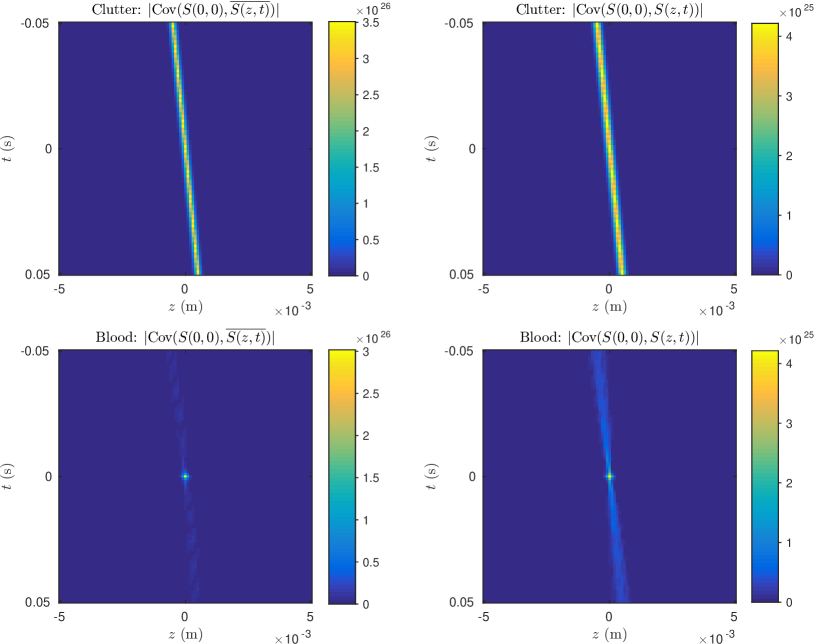
(c) Absolute values of the correlations in the clutter model (σ=0𝜎0\sigma=0, vc=102ms1subscript𝑣𝑐superscript102msuperscripts1v_{c}=10^{-2}\,\mathrm{m\!\cdot\!s^{-1}}) and in the blood model (σ2=106m2s1superscript𝜎2superscript106superscriptm2superscripts1\sigma^{2}=10^{-6}\,\mathrm{m^{2}s^{-1}}, vb=102ms1subscript𝑣𝑏superscript102msuperscripts1v_{b}=10^{-2}\,\mathrm{m\!\cdot\!s^{-1}}).
Figure 7: Correlations of the Casorati matrix.

On one hand, in the case of blood, since Cgg¯subscript𝐶𝑔¯𝑔C_{g\bar{g}} and Cggsubscript𝐶𝑔𝑔C_{gg} are oscillating and with very small support (see Figures 7a and 7b), the integration done when taking the expectation in the blood case should yield small correlations as long as |tjtj|subscript𝑡superscript𝑗subscript𝑡𝑗|t_{j^{\prime}}-t_{j}| is large enough. On the other hand, in the case of clutter, correlations will be high between the two signals as long as zizisubscript𝑧𝑖subscript𝑧superscript𝑖z_{i}-z_{i^{\prime}} and vc(tjtj)subscript𝑣𝑐subscript𝑡𝑗subscript𝑡superscript𝑗v_{c}\left(t_{j}-t_{j^{\prime}}\right) are of the same order and almost cancel out. This heuristic is confirmed by numerical experiments. In Figure 7c, we compare the clutter model and the blood model in one dimension: velocities are in the z𝑧z direction, and we only consider points aligned on the z𝑧z axis. As we can see, correlations are quickly decaying as we move away from (0,0)00(0,0) in the case of blood. In the case of clutter, there are correlations at any times at the corresponding displaced locations.

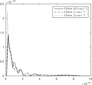
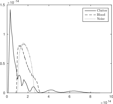
Once the correlation matrix is computed, we can generate a large number of samples to study the distribution of the singular values in different cases. In Figure 8a, we compare the distribution in the two models (blood and clutter), using the Gaussian limit approximation for the simulations, with the same intensity for both models. A comparison with a white noise model with the same variance shows that blood and noise have approximately the same singular value distribution. On the contrary, the distribution of the singular values of clutter presents a much larger tail. A comparison of the distribution of the singular values for the clutter model at different velocities shows no real difference in the tail of the distribution (Figure 8b).
Refer to caption
(a) The clutter model (σ=0𝜎0\sigma=0, vc=102ms1subscript𝑣𝑐superscript102msuperscripts1v_{c}=10^{-2}\,\mathrm{m\!\cdot\!s^{-1}}), the blood model (σ2=106m2s1superscript𝜎2superscript106superscriptm2superscripts1\sigma^{2}=10^{-6}\,\mathrm{m^{2}s^{-1}}, vb=102ms1subscript𝑣𝑏superscript102msuperscripts1v_{b}=10^{-2}\,\mathrm{m\!\cdot\!s^{-1}}) and a white noise model with same variance as the blood.
Refer to caption
(b) The clutter model with different velocities.
Figure 8: The distribution of the singular values of the Casorati matrix S𝑆S in different cases.

As a consequence, the clutter signal scsubscript𝑠𝑐s_{c} is well approximated by a low rank matrix, and the blood signal can be thought of as if it were only noise. Therefore, the SVD method act as a denoising algorithm and extracts the clutter signal, according to the discussion in the previous subsection.

6 Numerical Experiments

In this section, we consider again a more realistic 2D model, given by (17). This framework will allow us to simulate generic blood flow imaging sequences from particles. The dynamics of blood and clutter are modelled as follows. Let us assume that clutter is subject to a deterministic and computable flow φcsubscript𝜑𝑐\varphi_{c}. The randomness of the motion of red blood cells in vessels is modelled by a stochastic differential equation, given by

d𝐲=𝐯b(t,y)dt+σ(y)dBt,𝑑𝐲subscript𝐯𝑏𝑡𝑦𝑑𝑡𝜎𝑦𝑑subscript𝐵𝑡d\mathbf{y}=\mathbf{v}_{b}\left(t,y\right)dt+\sigma(y)\,dB_{t}, (24)

where Btsubscript𝐵𝑡B_{t} is a two dimensional Brownian motion and σ𝜎\sigma is determined by the effective diffusion coefficient K=12σ2𝐾12superscript𝜎2K=\frac{1}{2}\sigma^{2}. In blood vessels, this diffusion coefficient is proportional to the product γ˙r2˙𝛾superscript𝑟2\dot{\gamma}r^{2} where γ˙˙𝛾\dot{\gamma} is the shear stress in the vessel, and r𝑟r is the radius of red blood cells. As in the previous section, let ac=a1,csubscript𝑎𝑐subscript𝑎1𝑐a_{c}=a_{1,c} and ab=a1,bsubscript𝑎𝑏subscript𝑎1𝑏a_{b}=a_{1,b}. Let φbsubscript𝜑𝑏\varphi_{b} be the flow associated to (24). We assume that φbsubscript𝜑𝑏\varphi_{b} represents the dynamics of blood particles, relative to overall clutter movement, so that

ac(t)=φc(uc,t),φc(uc,0)=uc,formulae-sequencesubscript𝑎𝑐𝑡subscript𝜑𝑐subscript𝑢𝑐𝑡subscript𝜑𝑐subscript𝑢𝑐0subscript𝑢𝑐a_{c}\left(t\right)=\varphi_{c}\left(u_{c},t\right),\qquad\varphi_{c}(u_{c},0)=u_{c}, (25)

and

ab(t)=φc(φb(ub,t),t),φb(ub,0)=ub.formulae-sequencesubscript𝑎𝑏𝑡subscript𝜑𝑐subscript𝜑𝑏subscript𝑢𝑏𝑡𝑡subscript𝜑𝑏subscript𝑢𝑏0subscript𝑢𝑏a_{b}\left(t\right)=\varphi_{c}\left(\varphi_{b}\left(u_{b},t\right),t\right),\qquad\varphi_{b}(u_{b},0)=u_{b}. (26)

The dynamics of all the other particles are then taken to be independent realizations of the same dynamics. The velocity field 𝐯bsubscript𝐯𝑏\mathbf{v}_{b} and the clutter dynamics φcsubscript𝜑𝑐\varphi_{c} are computed beforehand and correspond to the general blood flow velocity and to an elastic displacement, respectively. In our experiments, we let φcsubscript𝜑𝑐\varphi_{c} be an affine displacement of the medium, changing over time: a global affine transformation, with slowly varying translation and shearing applied to the medium at each frame, namely

φc(u,t)=[1w1(t)01]u+[w2(t)w3(t)],subscript𝜑𝑐𝑢𝑡delimited-[]1subscript𝑤1𝑡01𝑢delimited-[]subscript𝑤2𝑡subscript𝑤3𝑡\varphi_{c}(u,t)=\left[\begin{smallmatrix}1&w_{1}(t)\\ 0&1\end{smallmatrix}\right]u+\left[\begin{smallmatrix}w_{2}(t)\\ w_{3}(t)\end{smallmatrix}\right],

where wisubscript𝑤𝑖w_{i} are smooth and slowly varying (compared to φbsubscript𝜑𝑏\varphi_{b}) functions such that wi(0)=0subscript𝑤𝑖00w_{i}(0)=0. As for the blood velocity flow 𝐯bsubscript𝐯𝑏\mathbf{v}_{b}, it is parallel to the blood vessels, with its intensity decreasing away from the center of the blood vessel [18, Section 11.3]. More precisely, 𝐯bsubscript𝐯𝑏\mathbf{v}_{b} is a Poiseuille laminar flow, namely the mean blood flow velocity is half of the maximum velocity, which is the fluid velocity in the center of the vessel.
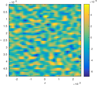
Refer to caption
Figure 9: Single frame of ultrafast ultrasound (real part).

The relative blood displacements bk,j=φk,b(ub,k,tj)subscript𝑏𝑘𝑗subscript𝜑𝑘𝑏subscript𝑢𝑏𝑘subscript𝑡𝑗b_{k,j}=\varphi_{k,b}\left(u_{b,k},t_{j}\right) are computed according to the following discretization of the stochastic differential equation (24):

bk,j+1=bk,j+δt𝐯b(tj,bk,j)+δtσ(bk,j)Xk,j+o(δt),subscript𝑏𝑘𝑗1subscript𝑏𝑘𝑗𝛿𝑡subscript𝐯𝑏subscript𝑡𝑗subscript𝑏𝑘𝑗𝛿𝑡𝜎subscript𝑏𝑘𝑗subscript𝑋𝑘𝑗𝑜𝛿𝑡b_{k,j+1}=b_{k,j}+\delta t\mathbf{v}_{b}\left(t_{j},b_{k,j}\right)+\sqrt{\delta t}\sigma\left(b_{k,j}\right)X_{k,j}+o\left(\delta t\right),

where (Xk,j)subscript𝑋𝑘𝑗\left(X_{k,j}\right) are centered independent Gaussian random variables and δt=tj+1tj𝛿𝑡subscript𝑡𝑗1subscript𝑡𝑗\delta t=t_{j+1}-t_{j} is taken to be constant. The blood particle positions ak,b(tj)subscript𝑎𝑘𝑏subscript𝑡𝑗a_{k,b}\left(t_{j}\right) are then computed simply by applying the precomputed flow φcsubscript𝜑𝑐\varphi_{c}.

Refer to caption
(a) Maximum blood velocity: 2cms12cmsuperscripts12\,\mathrm{cm\!\cdot\!s^{-1}}; mean clutter velocity: 1cms11cmsuperscripts11\,\mathrm{cm\!\cdot\!s^{-1}}.
Refer to caption
(b) Maximum blood velocity: 1cms11cmsuperscripts11\,\mathrm{cm\!\cdot\!s^{-1}}; mean clutter velocity: 1cms11cmsuperscripts11\,\mathrm{cm\!\cdot\!s^{-1}}.
Refer to caption
(c) Maximum blood velocity: 0.5cms10.5cmsuperscripts10.5\,\mathrm{cm\!\cdot\!s^{-1}}; mean clutter velocity: 1cms11cmsuperscripts11\,\mathrm{cm\!\cdot\!s^{-1}}.
Figure 10: The SVD method for different velocities and orientations. In each case, we have from left to right: the blood velocity and location, the reconstructed blood location, the decay of the singular values. The squares are 5mm×5mm5mm5mm5\,\mathrm{mm}\times 5\,\mathrm{mm}, and the horizontal and vertical axes are the x𝑥x and z𝑧z axes, respectively. The parameters used are those given in (1) and (2), F=0.4𝐹0.4F=0.4 and Θ=7°Θ7°\Theta=7\^{A}\textdegree. The density of particles for both blood and clutter is 2,000 per mm2superscriptmm2\mathrm{mm^{2}}, and σ=2.5105𝜎2.5superscript105\sigma=2.5\cdot 10^{-5}.

In order to validate the SVD approach, we explore the effects of the blood velocity and of the direction of the blood vessels on the behavior of the singular values and on the quality of the reconstruction. In each case, the clutter displacement is the same composition of time-varying shearing and translation, and the mean clutter velocity is 1cms11cmsuperscripts11\,\mathrm{cm\!\cdot\!s^{-1}}. We choose Cc=5subscript𝐶𝑐5C_{c}=5 and Cb=1subscript𝐶𝑏1C_{b}=1, for the same density of scatterers from clutter and blood: per unit of area, the clutter intensity is therefore five times higher than the blood intensity. A single frame of ultrafast ultrasound imaging is presented in Figure 9: it is clear that without further processing, it is impossible to locate the blood vessels.

In Figure 10, the results for various velocities and orientations are presented. The reconstruction intensities are expressed in decibels, relatively to the smallest value in the image. The SVD method allows for reconstruction of blood vessels, even if the maximum blood velocity is close to, or oven lower than, the mean velocity of clutter. We always use the threshold K=20𝐾20K=20. As we can see, due to the better resolution in the z𝑧z direction discussed in Section 3, vessels oriented parallel to the receptor array have a reconstruction with a better resolution. But due to the oscillating behavior of the PSF in the z𝑧z direction, and the low-pass filter behavior of the PSF in the x𝑥x direction, the sensitivity is better for vessels oriented perpendicularly to the receptor array, and the SVD method is able to reconstruct smaller vessels with lower velocities. This follows from the discussion in Subsection 4.2. In order to visualize this phenomenon even better, Figure 11 presents the time behavior of a single pixel from the data of Figure 10c. We can clearly see the doppler effect in the case when the flow is perpendicular to the receptor array, and the low frequency behavior of the signal in the case when it is parallel to the receptor array.
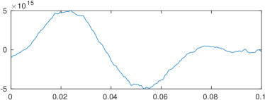
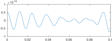
Refer to caption
(a) Flow parallel to the receptor array.
Refer to caption
(b) Flow perpendicular to the receptor array.
Figure 11: Time behavior of a single pixel (real part), located in a constant velocity flow.

In Figure 12, results of an investigation on the effect of the threshold K𝐾K on the reconstruction are presented. Except for K𝐾K, the parameters of Figure 10b are used. If the threshold is too low, the reconstruction is not satisfactory and artefacts appear everywhere in the reconstructed image. If the threshold is too high, the reconstruction still works but the contrast becomes lower. With our parameters, K=20𝐾20K=20 seems to produce the best results.
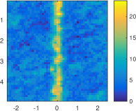
Refer to caption
(a) Flow parallel to the receptor array.
Refer to caption
(b) Flow perpendicular to the receptor array.
Figure 12: Effect of the threshold K𝐾K on the reconstruction. From left to right: K=10,20,30,40𝐾10203040{K=10,20,30,40}.
Refer to caption
(a) Contrast as a function of noise level
Refer to caption
(b) 0% noise
Refer to caption
(c) 2.5% noise
Refer to caption
(d) 5% noise
Refer to caption
(e) 7.5% noise
Figure 13: Effect of noise on the reconstruction. The parameters are the same used in Figure 10b.

In order to further validate the method, we consider the impact of measurement noise on the recovery. To this end, we add independent white Gaussian noise to the data, and consider the quality of the reconstruction as a function of the noise intensity. Let us define the contrast of the reconstruction as the ratio between the mean intensity of the reconstructed image inside and outside the blood domain. The parameters of Figure 10b are used. Blood intensity is five times lower than clutter intensity, and therefore a noise intensity of 10% corresponds to half the intensity of blood. In Figure 13, sample reconstructions at different noise levels are provided. We can conclude that contrast is robust to moderate levels of noise, since blood vessels can still be identified up to 7.5% of noise if they are oriented along the z axis, and up to 2.5% of noise if they are oriented along the x axis. Figure 13 also clearly quantifies the better contrast for vessels oriented along the z axis.

7 Concluding Remarks

In this paper, we have provided for the first time a detailed mathematical analysis of ultrafast ultrasound imaging. By using a random model for the movement of the blood cells, we have shown that an SVD approach can separate the blood signal from the clutter signal. Our model and results open a door for a mathematical and numerical framework for realizing super-resolution in dynamic optical coherence tomography [12], in ultrafast ultrasound imaging by tracking microbubbles [9], as well as in acousto-optic imaging based on the use of ultrasound plane waves instead of focused ones, which allows to increase the imaging rate drastically [13]. These three modalities are under investigation and their mathematical and numerical modeling will be the subject of forthcoming papers.

Appendix A The Justification of the Approximation of the PSF

This appendix is devoted to the formal justification of the PSF approximation (8) which was obtained by truncating the Taylor expansion of w±θsuperscriptsubscript𝑤plus-or-minus𝜃w_{\pm}^{\theta} at the first order: we shall show here that the error caused by this truncation is small. For simplicity, we shall consider only the case when z=z𝑧superscript𝑧z=z^{\prime} and θ=0𝜃0\theta=0: the general case may be tackled in a similar way. Without loss of generality, we may set x=0superscript𝑥0x^{\prime}=0 and suppose x0𝑥0x\geq 0. We also suppose that we are not too close to the detectors, namely z102m𝑧superscript102mz\geq 10^{-2}\,\mathrm{m}. Moreover, in order to be able to be quantitative, we consider the particular case when F=0.4𝐹0.4F=0.4 and τ=1𝜏1\tau=1.

The expression of the PSF that we want to approximate is (see (7))

g(x):=g0((x,z),(0,z))=c04πx[f(w+(x))f(w(x))],assign𝑔𝑥subscript𝑔0𝑥𝑧0𝑧subscript𝑐04𝜋𝑥delimited-[]superscript𝑓subscript𝑤𝑥superscript𝑓subscript𝑤𝑥g(x):=g_{0}((x,z),(0,z))=\frac{c_{0}}{4\pi x}\left[f^{\prime}(w_{+}(x))-f^{\prime}(w_{-}(x))\right],

where w±(x)subscript𝑤plus-or-minus𝑥w_{\pm}(x) is given by

w±(x):=h𝐱,𝐱0(x±Fz)=c01(1+F2zz2+(x±Fz)2).assignsubscript𝑤plus-or-minus𝑥superscriptsubscript𝐱superscript𝐱0plus-or-minus𝑥𝐹𝑧superscriptsubscript𝑐011superscript𝐹2𝑧superscript𝑧2superscriptplus-or-minus𝑥𝐹𝑧2w_{\pm}(x):=h_{\mathbf{x},\mathbf{x}^{\prime}}^{0}(x\pm Fz)=c_{0}^{-1}\left(\sqrt{1+F^{2}}z-\sqrt{z^{2}+(x\pm Fz)^{2}}\right).

(Note that, for simplicity of notation, we have removed the dependence of w𝑤w on θ𝜃\theta and z𝑧z.) An immediate calculation shows that

w±(0)=0,w±(0)=c01F1+F2,w±′′(x)=c01z2((x±Fz)2+z2)3/2.formulae-sequencesubscript𝑤plus-or-minus00formulae-sequencesubscriptsuperscript𝑤plus-or-minus0minus-or-plussuperscriptsubscript𝑐01𝐹1superscript𝐹2subscriptsuperscript𝑤′′plus-or-minus𝑥superscriptsubscript𝑐01superscript𝑧2superscriptsuperscriptplus-or-minus𝑥𝐹𝑧2superscript𝑧232w_{\pm}(0)=0,\qquad w^{\prime}_{\pm}(0)=\frac{\mp c_{0}^{-1}F}{\sqrt{1+F^{2}}},\qquad w^{\prime\prime}_{\pm}(x)=\frac{-c_{0}^{-1}z^{2}}{\left((x\pm Fz)^{2}+z^{2}\right)^{3/2}}.

Hence, there exists ξx[0,x]subscript𝜉𝑥0𝑥\xi_{x}\in[0,x] such that

w±(x)=c01F1+F2x+cxx22,|cx|=|w±′′(ξx)|c01z1.formulae-sequencesubscript𝑤plus-or-minus𝑥minus-or-plussuperscriptsubscript𝑐01𝐹1superscript𝐹2𝑥subscript𝑐𝑥superscript𝑥22subscript𝑐𝑥superscriptsubscript𝑤plus-or-minus′′subscript𝜉𝑥superscriptsubscript𝑐01superscript𝑧1w_{\pm}(x)=\frac{\mp c_{0}^{-1}F}{\sqrt{1+F^{2}}}x+c_{x}\frac{x^{2}}{2},\qquad|c_{x}|=|w_{\pm}^{\prime\prime}(\xi_{x})|\leq c_{0}^{-1}z^{-1}.

Therefore, the absolute error E(x)𝐸𝑥E(x) due to the truncation of the Taylor series of w±subscript𝑤plus-or-minusw_{\pm} at first order is given by

E(x)=c0(4π)1[E+(x)E(x)],𝐸𝑥subscript𝑐0superscript4𝜋1delimited-[]subscript𝐸𝑥subscript𝐸𝑥E(x)=c_{0}(4\pi)^{-1}\left[E_{+}(x)-E_{-}(x)\right],

where

E±(x)=1x[f(c01F1+F2x+cxx22)f(c01F1+F2x)].subscript𝐸plus-or-minus𝑥1𝑥delimited-[]superscript𝑓minus-or-plussuperscriptsubscript𝑐01𝐹1superscript𝐹2𝑥subscript𝑐𝑥superscript𝑥22superscript𝑓minus-or-plussuperscriptsubscript𝑐01𝐹1superscript𝐹2𝑥E_{\pm}(x)=\frac{1}{x}\left[f^{\prime}(\frac{\mp c_{0}^{-1}F}{\sqrt{1+F^{2}}}x+c_{x}\frac{x^{2}}{2})-f^{\prime}(\frac{\mp c_{0}^{-1}F}{\sqrt{1+F^{2}}}x)\right].

We now consider two cases, depending on x𝑥x. First, consider the case when x>5103m𝑥5superscript103mx>5\cdot 10^{-3}\,\mathrm{m}. From the above calculations we immediately have

|E(x)|c0(4π)14xf25c0103ν03.71012.𝐸𝑥subscript𝑐0superscript4𝜋14𝑥subscriptnormsuperscript𝑓25subscript𝑐0superscript103subscript𝜈03.7superscript1012|E(x)|\leq c_{0}(4\pi)^{-1}\frac{4}{x}\left\|f^{\prime}\right\|_{\infty}\leq\frac{2}{5}c_{0}10^{3}\nu_{0}\leq 3.7\cdot 10^{12}.

Next, consider the case when x5103m𝑥5superscript103mx\leq 5\cdot 10^{-3}\,\mathrm{m}. By using again the mean value theorem we obtain

E±(x)=cxx2f′′(θx),θx=c01F1+F2x+δxcxx22formulae-sequencesubscript𝐸plus-or-minus𝑥subscript𝑐𝑥𝑥2superscript𝑓′′subscript𝜃𝑥subscript𝜃𝑥minus-or-plussuperscriptsubscript𝑐01𝐹1superscript𝐹2𝑥subscript𝛿𝑥subscript𝑐𝑥superscript𝑥22E_{\pm}(x)=c_{x}\frac{x}{2}f^{\prime\prime}(\theta_{x}),\qquad\theta_{x}=\frac{\mp c_{0}^{-1}F}{\sqrt{1+F^{2}}}x+\delta_{x}c_{x}\frac{x^{2}}{2}

for some δx[0,1]subscript𝛿𝑥01\delta_{x}\in[0,1]. Since |f′′(t)|superscript𝑓′′𝑡|f^{\prime\prime}(t)| is even and decreasing for t>0𝑡0t>0, we have that

|E±(x)|c01x2z|f′′(c01F1+F2xc01x22z)|,subscript𝐸plus-or-minus𝑥superscriptsubscript𝑐01𝑥2𝑧superscript𝑓′′superscriptsubscript𝑐01𝐹1superscript𝐹2𝑥superscriptsubscript𝑐01superscript𝑥22𝑧|E_{\pm}(x)|\leq c_{0}^{-1}\frac{x}{2z}|f^{\prime\prime}(\frac{c_{0}^{-1}F}{\sqrt{1+F^{2}}}x-c_{0}^{-1}\frac{x^{2}}{2z})|,

since the inequality x5103m𝑥5superscript103mx\leq 5\cdot 10^{-3}\,\mathrm{m} guarantees that c01F1+F2xc01x22z>0superscriptsubscript𝑐01𝐹1superscript𝐹2𝑥superscriptsubscript𝑐01superscript𝑥22𝑧0\frac{c_{0}^{-1}F}{\sqrt{1+F^{2}}}x-c_{0}^{-1}\frac{x^{2}}{2z}>0. Therefore we have

|E(x)|(4π)1xz1|f′′(c01F1+F2xc01x22z)|.𝐸𝑥superscript4𝜋1𝑥superscript𝑧1superscript𝑓′′superscriptsubscript𝑐01𝐹1superscript𝐹2𝑥superscriptsubscript𝑐01superscript𝑥22𝑧|E(x)|\leq(4\pi)^{-1}xz^{-1}|f^{\prime\prime}(\frac{c_{0}^{-1}F}{\sqrt{1+F^{2}}}x-c_{0}^{-1}\frac{x^{2}}{2z})|.

Let us look at the right hand side of this inequality. As x0𝑥0x\to 0 the error tends to 00: this is expected, because of the Taylor expansion around 00. On the other hand, for big x𝑥x, the value of |f′′(c01F1+F2xc01x22z)|superscript𝑓′′superscriptsubscript𝑐01𝐹1superscript𝐹2𝑥superscriptsubscript𝑐01superscript𝑥22𝑧|f^{\prime\prime}(\frac{c_{0}^{-1}F}{\sqrt{1+F^{2}}}x-c_{0}^{-1}\frac{x^{2}}{2z})| is very small, since |f′′(t)|superscript𝑓′′𝑡|f^{\prime\prime}(t)| decays very rapidly for large t𝑡t. Therefore, the maximum of the right hand side is attained in a point x(0,0.005)superscript𝑥00.005x^{*}\in(0,0.005). The value in this point may be explicitly calculated, and we have

|E(x)|41012,0x5103m.formulae-sequence𝐸𝑥4superscript10120𝑥5superscript103m|E(x)|\leq 4\cdot 10^{12},\qquad 0\leq x\leq 5\cdot 10^{-3}\,\mathrm{m}.

To summarize the above derivation, we have shown that the absolute error E(x)𝐸𝑥E(x) is bounded by

|E(x)|41012,x0.formulae-sequence𝐸𝑥4superscript1012𝑥0|E(x)|\leq 4\cdot 10^{12},\qquad x\geq 0. (27)

We now wish to estimate the relative error E/gsubscriptnorm𝐸subscriptnorm𝑔\left\|E\right\|_{\infty}/\left\|g\right\|_{\infty}. In order to do this, let us compute g(0)𝑔0g(0). Since the Taylor expansion becomes exact as x0𝑥0x\to 0, we may very well compute g(0)𝑔0g(0) by using the approximated version. Thus, setting G=F/1+F2𝐺𝐹1superscript𝐹2G=F/\sqrt{1+F^{2}} we have

g(0)=limx0c04πx[f(c01Gx)f(c01Gx)]=limx0G(4π)1[f(c01Gx)f(0)c01Gx+f(c01Gx)f(0)c01Gx]=2G(4π)1f′′(0),𝑔0subscript𝑥0subscript𝑐04𝜋𝑥delimited-[]superscript𝑓superscriptsubscript𝑐01𝐺𝑥superscript𝑓superscriptsubscript𝑐01𝐺𝑥subscript𝑥0𝐺superscript4𝜋1delimited-[]superscript𝑓superscriptsubscript𝑐01𝐺𝑥superscript𝑓0superscriptsubscript𝑐01𝐺𝑥superscript𝑓superscriptsubscript𝑐01𝐺𝑥superscript𝑓0superscriptsubscript𝑐01𝐺𝑥2𝐺superscript4𝜋1superscript𝑓′′0\begin{split}g(0)&=\lim_{x\to 0}-\frac{c_{0}}{4\pi x}\left[f^{\prime}(c_{0}^{-1}Gx)-f^{\prime}(-c_{0}^{-1}Gx)\right]\\ &=\lim_{x\to 0}-G(4\pi)^{-1}\left[\frac{f^{\prime}(c_{0}^{-1}Gx)-f^{\prime}(0)}{c_{0}^{-1}Gx}+\frac{f^{\prime}(-c_{0}^{-1}Gx)-f^{\prime}(0)}{-c_{0}^{-1}Gx}\right]\\ &=-2G(4\pi)^{-1}f^{\prime\prime}(0),\end{split}

whence |g(0)|8.81013𝑔08.8superscript1013|g(0)|\geq 8.8\cdot 10^{13} by a direct calculation of |f′′(0)|superscript𝑓′′0|f^{\prime\prime}(0)|. Finally, combining this inequality with (27) allows to bound the relative error by

Eg5%.subscriptnorm𝐸subscriptnorm𝑔percent5\frac{\left\|E\right\|_{\infty}}{\left\|g\right\|_{\infty}}\leq 5\%.

We have proven that the relative error of the approximation obtained by truncating the Taylor expansions of w±subscript𝑤plus-or-minusw_{\pm} at the first order is less than 5%. This has been proven only in the particular case when z=z𝑧superscript𝑧z=z^{\prime}: the general case may be done by extending the above argument to two dimensions.

References

  • [1] H. Ammari, J. Garnier, W. Jing, H. Kang, M. Lim, K. Solna, and W. H. Mathematical and Statistical Methods for Multistatic Imaging, volume 2098 of Lecture Notes in Mathematics. Springer, Cham, 2013.
  • [2] J. Bercoff, G. Montaldo, T. Loupas, D. Savery, F. Meziere, M. Fink, and M. Tanter. Ultrafast compound doppler imaging: providing full blood flow characterization. IEEE Transactions on Ultrasonics, Ferroelectrics, and Frequency Control, 58(1):134–147, January 2011.
  • [3] S. Bjaerum, H. Torp, and K. Kristoffersen. Clutter filter design for ultrasound color flow imaging. IEEE Transactions on Ultrasonics, Ferroelectrics, and Frequency Control, 49(2):204–216, Feb 2002.
  • [4] A. v. d. Bos. The multivariate complex normal distribution-a generalization. IEEE Transactions on Information Theory, 41(2):537–539, 1995.
  • [5] C. Bruneel, R. Torguet, K. M. Rouvaen, E. Bridoux, and B. Nongaillard. Ultrafast echotomographic system using optical processing of ultrasonic signals. Applied Physics Letters, 30(8):371–373, 1977.
  • [6] C. G. Caro. The mechanics of the circulation. Cambridge University Press, 2012.
  • [7] W. C. Chew. Waves and fields in inhomogeneous media, volume 522. IEEE press New York, 1995.
  • [8] C. Demene, T. Deffieux, M. Pernot, B.-F. Osmanski, V. Biran, J.-L. Gennisson, L.-A. Sieu, A. Bergel, S. Franqui, J.-M. Correas, et al. Spatiotemporal clutter filtering of ultrafast ultrasound data highly increases doppler and fultrasound sensitivity. Medical Imaging, IEEE Transactions on, 34(11):2271–2285, 2015.
  • [9] C. Errico, J. Pierre, S. Pezet, Y. Desailly, Z. Lenkei, O. Couture, and M. Tanter. Ultrafast ultrasound localization microscopy for deep super-resolution vascular imaging. Nature, 527(7579):499–502, Nov 2015. Letter.
  • [10] J.-L. Gennisson, T. Deffieux, M. Fink, and M. Tanter. Ultrasound elastography: Principles and techniques. Diagnostic and Interventional Imaging, 94(5):487 – 495, 2013.
  • [11] K. Iizuka and P. Kmtky. Data adaptive signal estimation by singular value decomposition of data matrix. Proceedings of the IEEE, 70(6), 1982.
  • [12] C. Joo, C. Evans, T. Stepinac, T. Hasan, and J. de Boer. Diffusive and directional intracellular dynamics measured by field-based dynamic light scattering. OPTICS EXPRESS, 18(3):2858–2871, Jan 2010.
  • [13] J.-B. Laudereau, A. Grabar, M. Tanter, J.-L. Gennisson, and F. Ramaz. Ultrafast acousto-optic imaging with ultrasonic plane waves. OPTICS EXPRESS, 24(4):3774–3789, Feb 2016.
  • [14] E. Mace, G. Montaldo, I. Cohen, M. Baulac, M. Fink, and M. Tanter. Functional ultrasound imaging of the brain. Nat Meth, 8(8):662–664, Aug 2011.
  • [15] E. Mace, G. Montaldo, B. F. Osmanski, I. Cohen, M. Fink, and M. Tanter. Functional ultrasound imaging of the brain: theory and basic principles. IEEE Transactions on Ultrasonics, Ferroelectrics, and Frequency Control, 60(3):492–506, March 2013.
  • [16] G. Montaldo, M. Tanter, J. Bercoff, N. Benech, and M. Fink. Coherent plane-wave compounding for very high frame rate ultrasonography and transient elastography. Ultrasonics, Ferroelectrics, and Frequency Control, IEEE Transactions on, 56(3):489–506, March 2009.
  • [17] K. K. Shung. Diagnostic ultrasound: Imaging and blood flow measurements. CRC press, 2015.
  • [18] T. L. Szabo. Diagnostic Ultrasound Imaging: Inside Out. Academic Press, Boston, second edition, 2014.
  • [19] M. Tanter and M. Fink. Ultrafast imaging in biomedical ultrasound. IEEE Transactions on Ultrasonics, Ferroelectrics, and Frequency Control, 61(1):102–119, January 2014.
  • [20] K. Watanabe. Integral transform techniques for Green’s function, volume 76 of Lecture Notes in Applied and Computational Mechanics. Springer, Cham, second edition, 2015.