Deep Learning for Short-Term Traffic Flow Prediction

Abstract

We develop a deep learning model to predict traffic flows. The main contribution is development of an architecture that combines a linear model that is fitted using $\ell_{1}$ regularization and a sequence of $\tanh$ layers. The challenge of predicting traffic flows are the sharp nonlinearities due to transitions between free flow, breakdown, recovery and congestion. We show that deep learning architectures can capture these nonlinear spatio-temporal effects. The first layer identifies spatio-temporal relations among predictors and other layers model nonlinear relations. We illustrate our methodology on road sensor data from Interstate I-55 and predict traffic flows during two special events; a Chicago Bears football game and an extreme snowstorm event. Both cases have sharp traffic flow regime changes, occurring very suddenly, and we show how deep learning provides precise short term traffic flow predictions.

1 Introduction

1.1 Traffic Flow Prediction

Real-time spatio-temporal measurements of traffic flow speed are available from in-ground loop detectors or GPS probes. Commercial traffic data providers, such as Bing maps Microsoft Research [2016], rely on traffic flow data, and machine learning to predict speeds for each road segment. Real-time (15-40 minute) forecasting gives travelers the ability to choose better routes and authorities the ability to manage the transportation system. Deep learning is a form of machine learning which provides good short-term forecasts of traffic flows by exploiting the dependency in the high dimensional set of explanatory variables, we capture the sharp discontinuities in traffic flow that arise in large-scale networks. We provide a variable selection methodology based on sparse models and dropout.

The goal of our paper is to model the nonlinear spatio-temporal effects in recurrent and non-recurrent traffic congestion patterns. These arise due to conditions at construction zones, weather, special events, and traffic incidents. Quantifying travel time uncertainty requires real-time forecasts. Traffic managers use model-based forecasts to regulate ramp metering, apply speed harmonization, and regulate road pricing as a congestion mitigation strategy; whereas, the general public adjusts travel decisions on departure times and travel route choices, among other things.

Deep learning forecasts congestion propagation given a bottleneck location, and can provide an accurate forty minute forecasts for days with recurrent and non-recurrent traffic conditions. Deep learning can also incorporate other data sources, such as weather forecasts, and police reports to produce more accurate forecasts. We illustrate our methodology on traffic flows during two special events; a Chicago Bears football game and an extreme snow storm event.

To perform variable selection, we develop a hierarchical sparse vector auto-regressive technique Dellaportas et al. [2012], Nicholson et al. [2014] as the first deep layer. Predictor selection then proceeds in a dropout Hinton and Salakhutdinov [2006]. Deep learning models the sharp discontinuities in traffic flow are modeled as a superposition of univariate non-linear activation functions with affine arguments. Our procedure is scalable and estimation follows traditional optimization techniques, such as stochastic gradient descent.

The rest of our paper is outlined as follows. Section 1.2 discusses connections with existing work. Section 1.3 reviews fundamentals of deep learning. Section 2 develops deep learning predictors for forecasting traffic flows. Section 3 discusses fundamental characteristics of traffic flow data and illustrates our methodology with the study of traffic flow on Chicago’s I-55. Finally, Section 4 concludes with directions for future research.

1.2 Connections with Existing Work

Short-term traffic flow prediction has a long history in the transportation literature. Deep learning is a form of machine learning that can be viewed as a nested hierarchical model which includes traditional neural networks. Karlaftis and Vlahogianni [2011] provides an overview of traditional neural network approaches and Kamarianakis et al. [2012a] shows that model training is computationally expensive with frequent updating being prohibitive. On the other hand, deep learning with dropout can find a sparse model which can be frequently updated in real time. There are several analytical approaches to traffic flows modeling Anacleto et al. [2013], Blandin et al. [2012], Chiou et al. [2014], Polson and Sokolov [2014, 2015], Work et al. [2010]. These approaches can perform very well on filtering and state estimation. The caveat is that they are hard to implement on large scale networks. Bayesian approaches have been shown to be efficient for handling large scale transportation network state estimation problems Tebaldi and West [1998]. Westgate et al. [2013] discusses ambulance travel time reliability using noisy GPS for both path travel time and individual road segment travel time distributions. Anacleto et al. [2013] provides a dynamic Bayesian network to model external intervention techniques to accommodate situations with suddenly changing traffic variables.

Statistical and machine learning methods for traffic forecasting are compared in  Smith and Demetsky [1997]. Sun et al. [2006] provides a Bayes network algorithm, where the conditional probability of a traffic state on a given road, given states on topological neighbors on a road network is calculated. The resulting joint probability distribution is a mixture of Gaussians. Bayes networks for estimating travel times were suggested by Horvitz et al. [2012] which eventually became a commercial product that led to the start of Inrix, a traffic data company. Wu et al. [2004] provides a machine-learning method support vector machine (SVM) Polson and Scott [2011] to forecast travel times and Quek et al. [2006] proposes a fuzzy neural-network approach to address nonlinearities in traffic data. Rice and van Zwet [2004] argues that there is a linear relation between future travel times and currently estimated conditions with a time-varying coefficients regression model to predict travel times.

Integrated auto-regressive moving average (ARIMA) and exponential smoothing (ES) for traffic forecasting are studied in Tan et al. [2009] and Van Der Voort et al. [1996]. A Kohonen self-organizing map is proposed as an initial classifier. Van Lint [2008] addresses real-time parameter learning and improves the quality of forecasts using an extended Kalman filter. Ban et al. [2011] proposes a method for estimating queue lengths at controlled intersections, based on the travel time data measured by GPS probes. The method relies on detecting discontinuities and changes of slopes in travel time data. Ramezani and Geroliminis [2015] combines the traffic flow shockwave analysis with data mining techniques. Oswald et al. [2000] argues that non-parametric methods produce better forecasts than parametric models due to their ability to better capture spatial-temporal relations and non-linear effects. Vlahogianni et al. [2014] provides an extensive recent review of literature on short-term traffic predictions.

There are several issues not addressed in the current literature Vlahogianni et al. [2014]. First, predictions at a network level using data-driven approaches. There are two situations when a data-driven approach might be preferable to methodologies based on traffic flow equations. Estimating boundary conditions is a challenging task, which even in systems that rely on loop detectors as traffic sensors are typically not installed on ramps. Missing data problems are usually addressed using data imputation Muralidharan and Horowitz [2009] or weak formulations of boundary conditions Strub and Bayen [2006]. Our results show that a data-driven approach can efficiently forecast flows without boundary measurements from ramps. Another challenge with physics-based approaches comes from their limited ability to model urban arterials. For example, Qiao et al. [2001] shows analytical approaches fail to provide good forecasts. Another challenge is to identify spatio-temporal relations in flow patterns, Vlahogianni et al. [2014] for further discussion. Data-driven approaches provide a flexible alternative to physical laws of traffic flows.

The challenge is to perform model selection and residual diagnostics Vlahogianni et al. [2014]. Model selection can be tackled by regularizing the loss function and using cross-validation to select the optimal penalty weight. To address this issue, when we specify our deep learning model we construct an architecture as follows. First we use is a regularized vector autoregressive model to perform predictor selection. Then, our deep learning model addresses the issue of non-linear and non-stationary relations between variables (speed measurements) using a series of activation functions.

Breiman Breiman [2003] describes the trade-off between machine learning and traditional statistical methods. Mchine learning has been widely applied Ripley [1996] and shown to be particularly successful in traffic pattern recognition. For example, shallow neural networks for traffic applications Chen and Grant-Muller [2001], use a memory efficient dynamic neural network based on resource allocating network (RAN) with a single hidden layer with Gaussian radial basis function activation unit. Zheng et al. [2006] develops several one-hidden layer networks to produce fifteen-minute forecasts. Two types of networks, one with a $\tanh$ activation function and one with a Gaussian radial basis function were developed. Several forecasts were combined using a Bayes factors that calculates an odds ratio for each of the models dynamically. Van Lint et al. [2005] proposes a state-space neural network and a multiple hypothesis approach that relies on using several neural network models at the same time van Hinsbergen et al. [2009]. Day of the week and time of day as inputs to a neural network was proposed in Çetiner et al. [2010]. Our work is closely related to Lv et al. [2015], which demonstrates that deep learning can be effective for traffic forecasts. A stacked auto-encoder was used to learn the spatial-temporal patterns in the traffic data with training performed by a greedy layer-wise fashion. Ma et al. [2015] proposed a recurrent architecture, a Long Short-Term Memory Neural Network (LSTM), for travel speed prediction. Our approach builds on this by showing an additional advantage of deeper hidden layers together with sparse autoregressive techniques for variable selection.

1.3 Deep Learning

Deep learning learns a high dimensional function via a sequence of semi-affine non-linear transformations. The deep architecture is organized as a graph. The nodes of the graph are units, connected by links to propagate activation, calculated at the origin, to the destination units. Each link has a weight that determines the relative strength and sign of the connection and each unit applies an activation function to all of the weighted sum of incoming activations. The activation function is given, such as a hard threshold, a sigmoid function or a $\tanh$. A particular class of deep learning models uses a directed acyclic graph structure is called a feed-forward neural network. There is vast literature on this topic; one of the earlier works include Bishop [1995] Haykin [2004].

Deep learning allows for efficient modeling of nonlinear functions, see the original problem of Poincare and Hilbert. The advantage of deep hidden layers is for a high dimensional input variable, $x=(x_{1},\ldots,x_{p})$ is that the activation functions are univariate, which implicitly requires the specification of the number of hidden units $N_{l}$ for each layer $l$.

The Kolmogorov-Arnold representation theorem Kolmogorov [1956] provides the theoretical motivation for deep learning. The theorem states that any continuous function of $n$ variables, defined by $F(x)$, can be represented as

$$F(x)=\sum_{j=1}^{2n+1}g_{j}\left(\sum_{i=1}^{n}h_{ij}(x_{i})\right),$$

where $g_{j}$ and $h_{ij}$ are continuous functions, and $h_{ij}$ is a universal basis, that does not depend on $F$. This remarkable representation result implies that any continuous function can be represented using operations of summation and function composition. For a neural network, it means that any function of $n$ variables can be represented as a neural network with one hidden layer and $2n+1$ activation units. The difference between theorem and neural network representations is that functions $h_{ij}$ are not necessarily affine. Much research has focused on how to find such a basis. In their original work, Kolmogorov and Arnold develop functions in a constructive fashion. Diaconis and Shahshahani [1984] characterizes projection pursuit functions for a specific types of input functions.

A deep learning predictor, denoted by $\hat{y}(x)$, takes an input vector $x=(x_{1},\ldots,x_{p})$ and outputs $y$ via different layers of abstraction that employ hierarchical predictors by composing $L$ non-linear semi-affine transformations. Specifically, a deep learning architecture is as follows. Let $f_{1},\ldots f_{n}$ be given univariate activation link functions, e.g. sigmoid ($1/(1+e^{-x})$, $\cosh(x)$, $\tanh(x)$), Heaviside gate functions ($I(x>0)$), or rectified linear units ($\max\{x,0\}$) or indicator functions ($I(x\in R)$) for trees. The composite map is defined by

$$\hat{y}(x):=F(x)=\left(f_{w_{n},b_{n}}\circ\ldots\circ f_{w_{1},b_{1}}\right)(x),$$

where $f_{w,b}$ is a semi-activation rule defined by

$$f_{w_{l},b_{l}}(x)=f\left(\sum_{j=1}^{N_{l}}w_{lj}x_{j}+b_{l}\right)=f(w_{l}^{T}x_{l}+b_{l})\quad(l=1,\ldots,n).$$ (1)

Here $N_{l}$ denotes the number of units at layer $l$. The weights $w_{l}\in R^{N_{l}\times N_{l-1}}$ and offset $b\in R$ needs to be learned from training data.

Data dimension reduction of a high dimensional map $F$ is performed via the composition of univariate semi-affine functions. Let $z^{l}$ denote the $l$-th layer hidden features, with $x=z^{0}$. The final output is the response $y$, can be numeric or categorical. The explicit structure of a deep prediction rule is than

$$z^{1}= f(w_{0}^{T}x+b_{0})$$

$$z^{2}= f(w_{1}^{T}z^{1}+b_{1})$$

$$\cdots$$

$$z^{q}= f(w_{n-1}^{T}z^{n-1}+b_{n-1})$$

$$y(x)= w_{n}^{T}z^{n}+b_{n}.$$

In many cases there is an underlying probabilistic models, denoted by $p(y\mid\hat{y}(x))$. This leads to a training problem given by optimization problem

$$\min_{w,b}\quad\dfrac{1}{T}\sum_{i=1}^{T}-\log p(y_{i}\mid\hat{y}_{w,b}(x_{i})),$$

where $p(y_{i}\mid\hat{y}(x))$ is the probability density function given by specification $y_{i}=F(x_{i})+\epsilon_{i}.$ For example, if $\epsilon_{i}$ is normal, we will be training $\hat{w},~{}\hat{b}$ via an $\ell_{2}$-norm, $\min_{w,b}||y-F_{w,b}(x)||^{2}=\sum_{i=1}^{T}(y_{i}-F_{w,b}(x_{i}))^{2}$. One of the key advantages of deep learning is the the derivative information $\nabla_{w,b}l(y,\hat{y}_{w,b}(x))$ is available in closed form via the chain rule. Typically, a regularization penalty, defined by $\lambda\phi(w,b)$ is added, to introduce the bias-variance decomposition to provide good out-of-sample predictive performance. An optimal regularization parameter, $\lambda$, can be chosen using out-of-sample cross-validation techniques. One of the advantages of $\ell_{1}$ penalized least squares formulation is that it leads to a convex, though non-smooth, optimization problem. Efficient algorithms Kim et al. [2007] exist to solve those problems, even for high dimensional cases.

There is a strong connection with nonlinear multivariate non-parametric models, which we now explore. In a traditional statistical framework, the non-parametric approach seeks to approximate the unknown map $F$ using a family of functions defined by the following expression

$$F(x)=\sum_{k=n}^{N}w_{k}f_{k}(x).$$ (2)

Functions $f_{k}$ are called basis functions and play the similar role of a functional space basis, i.e. they are chosen to give a good approximation to the unknown map $F$. In some cases $\{f_{k}\}_{k=1}^{N}$ actually do form a basis of a space, e.g., Fourier ($f_{k}(x)=\cos(kx)$) and wavelet bases. Multi-variate basis functions are usually constructed using functions of a single variable. Four examples are radial functions, ridge functions, kernel functions and indicator functions.

$$f_{k}(x)=\begin{cases}\kappa\left(||X-\gamma_{k}||_{2}\right)\mbox{ (radial function)}\\ \kappa(w^{T}X+w_{0})\mbox{ (ridge function)}\\ \kappa\left(\frac{X-\gamma_{k}}{h}\right)\mbox{ (kernel estimator)}\\ I(X\in C_{k})\mbox{ (tree indicator function)}\end{cases}$$ (3)

Here $\kappa$ is typically chosen to be a bell-shaped function (e.g., $1/e^{x^{2}}$ or $1/\cosh(x)$). The ridge function, a composition of inner-product and non-linear univariate functions, is arguably one of the simplest non-linear multi-variate function. Two of the most popular types of neural networks are constructed as a composition of radial or ridge functions. Popular non-parametric tree-based models Breiman et al. [1984] can be represented as (2) by choosing $f_{k}$ given by equation 3. In tree-based regression, weights $\alpha_{k}=\bar{Y}_{k}$ are the averages of $(Y_{i}\mid X_{i}\in C_{k})$ and $C_{k}$ is a box set in $R^{p}$ with zero or more extreme directions (open sides).

Another set of basis functions are Fourier series, used primarily for time series analysis, where $f_{k}(x)=\cos(x)$. A spline approximation can also be derived by using polinomial functions with finite support as a basis.

Ridge-based models, can efficiently represent high-dimensional data sets with a small number of parameters. We can think of deep features (outputs of hidden layers) as projections of the input data into a lower dimensional space. Deep learners can deal with the curse of dimensionality because ridge functions determine directions in $(z^{k-1},z^{k})$ input space, where the variance is very high. Those directions are chosen as global ones and represent the most significant patterns in the data. This approach resembles the other well-studied techniques such as projection pursuit Friedman and Tukey [1974] and principal component analysis.

2 Deep Learning for Traffic Flow Prediction

Let $x_{t+h}^{t}$ be the forecast of traffic flow speeds at time $t+h$, given measurements up to time $t$. Our deep learning traffic architecture looks like

$$y(x):=x_{t+40}^{t}=\left(\begin{array}[]{c}x_{1,t+40}\\ \vdots\\ x_{n,t+40}\end{array}\right).$$

To model traffic flow data $x^{t}=(x_{t-k},\ldots,x_{t})$ we use predictors $x$ given by

$$x^{t}=\mathrm{vec}\left(\begin{array}[]{ccc}x_{1,t-40}&...&x_{1,t}\\ \vdots&\vdots&\vdots\\ x_{n,t-40}&...&x_{n,t}\end{array}\right).$$

Here $n$ is the number of locations on the network (loop detectors) and $x_{i,t}$ is the cross-section traffic flow speed at location $i$ at time $t$. We use, vec to dennote the vectorization transformation, which converts the matrix into a column vector. In our application examined later in Section 3.1, we use twenty-one road segments (i.e., $n=21$) which span thirteen miles of a major corridor connecting Chicago’s southwest suburbs to the central business district. The chosen length is consistent with several current transportation corridor management deployments TransNet [2016].

Our layers are constructed as follows, $x=z^{0}$, then $z^{l+1}$, $l=0,\ldots,L$ is a time series “filter" given by

$$z_{i}^{l+1}= f\left(\sum_{i=1}^{N_{l}}\left(w_{i}^{l+1}z_{i}^{l}+b_{i}^{l+1}\right)\right)\quad(i=1,\ldots,N_{l+1}).$$

As we show later in out empirical studies, the problem of non-linearities in the data is efficiently addressed by the deep learners.

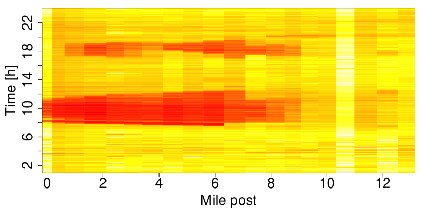
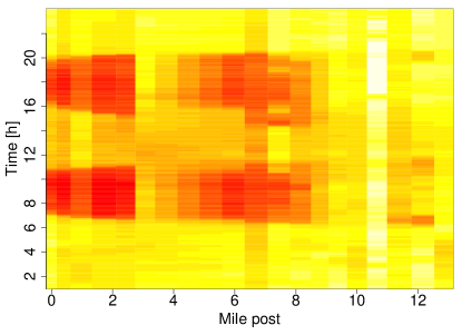
The problem of finding the spatio-temporal relations in the data is the predictor selection problem. Figure 1 shows a time-space diagram of traffic flows on a 13-mile stretch of highway I-55 in Chicago. You can see a clear spatio-temporal pattern in traffic congestion propagation in both downstream and upstream directions.

Figure 1: A time-space diagram that shows traffic flow speed on a 13-mile stretch of I-55. Cross-section speed measured on from 18 February 2009 (Wednesday). Red means slow speed and light yellow corresponds to free flow speed. The direction of the flow is from 0 to 13.

A predictor selection problem requires an algorithm to find a sparse models. Those rely on adding a penalty term to the loss function. A recent review by Nicholson et al. [2014] considers several prominent scalar regularization terms to identify sparse vector auto-regressive models.

Our approach will be to develop a hierarchical linear vector autoregressive model to identify the spatio-temporal relations in the data. We consider the problem of finding sparse matrix, $A$, in the following model

$$x_{t+40}^{t}=Ax^{t}+\epsilon_{t},\quad\epsilon_{t}\sim N(0,V);$$

where $A$ is a matrix of size $n\times nk$, and $k$ is the number of previous measurements used to develop a forecast. In our example in Section 3.1, we have $n=21$; however, in large scale networks, there are tens of thousands locations with measurements available.

The predictors selected as a result of finding the sparse linear model at the first layer are then used to build a deep learning model. To find an optimal network (structure and weights) we used the stochastic gradient descent (SGD) method implemented in the package H2O. Similar methods are available in Python’s Theano Bastien et al. [2012] or TensorFlow Abadi et al. [2016] framework. We use random search to find meta parameters of the deep learning model. To illustrate our methodology, we generated $N=10^{5}$ Monte Carlo samples from the following space:

$$f \in\{\tanh(x),~{}\max(x,0)\}$$

$$n \in\{1,\ldots,60\}$$

$$N_{l} \in\{1,\ldots,200\}^{n}$$

$$\lambda \in[10^{-4},~{}10^{-2}]$$

$$x_{t+h}^{t} =\left(f_{n}\circ\ldots\circ f_{1}\right)(x^{t}),\quad f_{l}=f(w_{l}^{T}x_{l}+b_{l}).$$

We used out-of-sample model performance as a criteria for selecting our final deep learning architecture.

2.1 Training

At a fundamental level, we use a training set $(y_{i},x_{i})_{i=1}^{N}$ of input-output pairs, to train our deep learning model by minimizing the difference between training target $y_{i}$ and our predictor $\hat{y}(x_{i})$. To do this, we require a loss function, $l(y,\hat{y})$ at the level of the output signal that measures our goodness-of-fit. When we have a traditional probabilistic model $p(y\mid\hat{y})$ that generates the output $y$ given the predictor $\hat{y}$, than we have the natural loss function $l(y,\hat{y})=-\log p(y~{}|~{}\hat{y})$. For deep learning problems, a typical $\ell_{2}$ norm squared used as a loss function. It is common to add a regularization penalty $\phi(w,b)$ that will avoid over-fitting and stabilize our predictive rule. To summarize, given an activation function, the statistical problem is to optimally find the weights and biases $w=(w_{0},\ldots,w_{n})$, $b=(b_{0},\ldots,b_{n})$ that minimize the loss function with $\ell_{2}$ separable regularization term given by

$$(\hat{w},~{}\hat{b})\in \operatorname*{argmin}_{w,b}~{}\|y-\hat{y}_{w,b}(x)\|_{2}^{2}+\lambda\phi(w,b)$$

$$\phi(w,b)= ||w||^{2}+||b||^{2}$$

$$\hat{y}_{w,b}(x)= \left(f_{n}\circ\ldots\circ f_{1}\right)(x^{t}),\quad f_{l}(x)=f\left(\sum_{j=1}^{n_{l}}w_{lj}x_{j}+b_{l}\right),$$

here $w_{l}\in\mathbb{R}^{n_{l}}$, $b_{l}\in\mathbb{R}$, and $\lambda$ gages the overall level of regularization. Choices of penalties for $\phi(w,b)$ include the ridge penalty $\ell_{2}$ or the lasso $\ell_{1}$ penalty to induce sparsity in the weights. A typical method to solve the optimization problem is stochastic gradient descent with mini-batches. The caveat of this approach include poor treatment of multi-modality and possibly slow convergence. From our experiments with the traffic data, we found that using sparse linear model estimation to identify spatial-temporal relations between variables yields better results, as compared to using dropout or regularization terms for neural network loss function Pachitariu and Sahani [2013], Helmbold and Long [2015]. Both penalized fitting and dropout Srivastava et al. [2014] are techniques for preventing overfitting. They control the bias-variance trade-off and improve out-of-sample performance of a model. A regularized model is less likely to overfit and will have a smaller size. Dropout considers all possible combinations of parameters by randomly dropping a unit out. Instead of considering different networks with different units being dropped out, a single network is trained with some probability of each unit being dropped out. Then during testing, the weights are scaled down according to drop-out probability to ensure that expected output is the same as actual output at the test time. Dropout is a heuristic method that is little understood but was shown to be very successful in practice. There is a deep connection though between penalized fitting for generalized linear models and dropout technique. Wager et al. [2013] showed that dropout is a first order equivalent to $\ell_{2}$ penalization after scaling the input data by the Fisher information matrix. For traffic flow prediction, there are predictors that are irrelevant, such as changes in traffic flow in a far away location that happened five minutes ago do not carry any information. Thus, by zeroing-out those predictors, the $\ell_{1}$ penalization leads to the sparsity pattern that better capture the spatio-temporal relations. A similar observation has been made in Kamarianakis et al. [2012b].

In order to find an optimal structure of the neural network (number of hidden layers $L$, number of activation units in each layer $N_{l}$ and activation functions $f$) as well as hyper-parameters, such as $\ell_{1}$ regularization weight, we used a random search. Though this technique can be inefficient for large scale problems, for the sake of exploring potential structures of the networks that deliver good results and can be scaled, this is an appropriate technique for small dimensions. Stochastic gradient descent used for training a deep learning model scales linearly with the data size. Thus the hyper-parameter search time is linear with respect to model size and data size. On a modern processor it takes about two minutes to train a deep learning network on 25,000 observations of 120 variables. To perform a hyper-parameter and model structure search we fit the model $10^{5}$ times. Thus the total wall-time (time that elapses from start to end) was 138 days. An alternative to random search for learning the network structure for traffic forecasts was proposed in Vlahogianni et al. [2005] and relies on the genetic optimization algorithm.

2.2 Trend Filtering

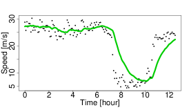
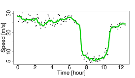
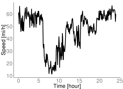
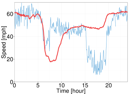
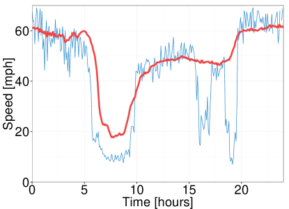
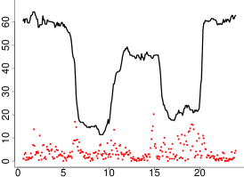
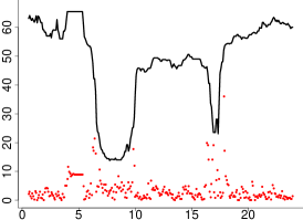
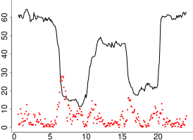
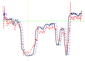
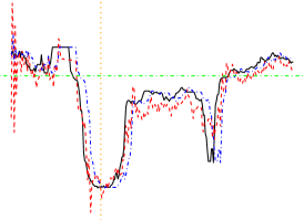
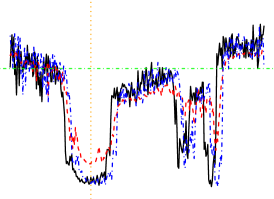
One goal of traffic flow modeling is to filter noisy data from physical sensors and then to develop model-based predictors. Iterative exponential smoothing is a popular technique that is computationally efficient. It smoothers oscillations that occur on arterial roads with traffic signal controls, when measured speed is “flipping” between two values, depending whether the probe vehicle stopped at the light or not. Figure 2(a), however, shows that it does not work well for quickly switching regimes observed in highway traffic. Another approach is median filtering, which unlike exponential smoothing captures quick changes in regimes as shown on Figure 2(b). However, it will not perform well on an arterial road controlled by traffic signals, since it will be oscillating back and forth between two values. A third approach is to use a piecewise polynomial fit to filter the data. Figure 2(c) shows that this method does perform well, as the slopes be underestimated. Median filtering seems to be the most effective in our context of traffic flows.

(a) exponential smoothing	(b) median filter	(c) loess filter

Figure 2: Results of three classical filtering techniques applied to traffic data (cross-section speed) from one of the work days.

An alternative approach to filter the data is to assume that we observe data from the statistical model $v_{i}=f(x_{i})+e_{i}$ , where $f(x)$ is piecewise constant. The fused lasso Tibshirani and Taylor [2011] and $\ell_{1}$ trend filtering Kim et al. [2009], Polson and Scott [2015] involves estimating $f(x)=(f(x_{1}),\ldots,f(x_{n}))$ at the input points by solving the optimization problem

$$\operatorname*{minimize}\quad||y-f(x)||_{2}^{2}+\lambda||Df(x)||_{1}.$$

In fused lasso $D=D^{(1)}$ is the matrix encoding first differences in $f(x)$. In $\ell_{1}$ trend filtering $D=D^{(2)}$ is the matrix encoding second differences in $f(x)$

$$D^{(1)}=\left(\begin{array}[]{cccccc}1&-1&0&0&\cdots&0\\ 0&1&-1&0&\cdots&0\\ \vdots&&&&\ddots&\vdots\\ 0&\cdots&&0&1&-1\end{array}\right),\quad D^{(2)}=\left(\begin{array}[]{cccccc}1&-2&1&0&\cdots&0\\ 0&1&-2&1&\cdots&0\\ \vdots&&&&\ddots&\vdots\\ 0&\cdots&&1&-2&1\end{array}\right).$$

Applying $D^{(1)}$ to a vector is equivalent to calculating first order differences of the vector. This filter also called 1-dimensional total variation denoising Rudin et al. [1992], and hence first order $\ell_{1}$ trend filtering estimate $f(x)$ is piecewise constant across the input points $x_{1},\ldots,x_{n}$. Higher orders difference operators $D^{(k)}$, $k>1$, correspond to an assumption that the data generating process is modeled by a piece-wise polynomial of order $k$ function.

The non-negative parameter, $\lambda$, controls the trade-off between smoothness of the signal and closeness to the original signal. The objective function is strictly convex and thus can be efficiently solved to find a unique minimizer $x^{\mathrm{lt}}$. The main reason to use the trend filtering is that it produces a piece-wise linear function in $t$. There are integer times, $1=t_{1}<t_{2},...,<t_{p}=n$ for which

$$x^{\mathrm{lt}}=\alpha_{k}+\beta_{k}t,~{}~{}t_{k}\leq t\leq t_{k+1},~{}~{}k=1,\ldots,p-1$$

Piece-wise linearity is guaranteed by using the $\ell_{1}$-norm penalty term. It guarantees sparseness of $Df(x)$ (the second-order difference of the estimated trend), i.e. it will have many zero elements, which means that the estimated trend is piecewise linear. The points $t_{2},\ldots,t_{p-1}$ are called kink points. The kink points correspond to change in slope and intercept of the estimated trend and can be interpreted as points at which regime of data generating process changes. This function well aligns with the traffic data from an in-ground sensor. The regimes in data correspond to free flow, degradation, congestion and recovery. Empirically, the assumption that data is piecewise linear is well justified. Residuals of the filtered data $x^{\mathrm{lt}}-y$ are typically low and show no patterns.

A trend filter is similar to a spline fitting method with one important difference. When we fit a spline (piece-wise continuous polynomial function) to the data, we need to provide knots (kinks) as inputs. Trend filtering has the advantage that the kinks and parameters of each line are found jointly.

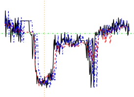
Figure 3 shows results of applying $\ell_{1}$ trend filter to a data measured from a loop-detector on I-55.

Figure 3: $\ell_{1}$ trend filtering based on quadratic loss and penalty that enforces a piecewise line fit applied to one day of measured cross-section speed.

A computationally efficient algorithms for trend filtering with differentiation operator of any order $D^{(k)}$ was recently proposed by Ramdas and Tibshirani [2015].

3 Chicago Traffic Flow During Special Events

To illustrate our methodology, we use data from twenty-one loop-detectors installed on a northbound section of Interstate I-55 . Those loop-detectors span 13 miles of the highway. Traffic flow data is available from the Illinois Department of Transportation, (see Lake Michigan Interstate Gateway Alliance http://www.travelmidwest.com/, formally the Gary-Chicago-Milwaukee Corridor, or GCM). The data is measured by loop-detector sensors installed on interstate highways. Loop-detector is a simple presence sensors that measure when a vehicle is present and generate an on/off signal. There are over 900 loop-detector sensors that cover the Chicago metropolitan area. Since 2008, Argonne National Laboratory has been archiving traffic flow data every five minutes from the grid of sensors. Data contains averaged speed, flow, and occupancy. Occupancy is defined as percent of time a point on the road is occupied by a vehicle, and flow is the number of off-on switches. Illinois uses a single loop detector setting, and speed is estimated based on the assumption of an average vehicle length.

A distinct characteristic of traffic flow data is an abrupt change of the mean level. Also we see a lot of variations on the speed measurements. Though, on Figure 2, it might seem that during the congested period (6am – 9am) the speed variation is small; in reality the signal to noise ratio during congested regime is lower compared to a free flow regime. One approach to treat the noisy data is a probabilistic one. In Polson and Sokolov [2014] the authors develop a hierarchical Bayesian model for tracking traffic flows and estimate uncertainty about state variables at any given point in time. However, when information is presented to a user, it has to be presented as a single number, i.e. travel time from my origin to my destination is 20 minutes. A straightforward way to move from a distribution over a traffic state variable (i.e., traffic flow speed) to a single number is to calculate an expected value or a maximum a posteriori.

3.1 Traffic Flow on Chicago’s Interstate I-55

One of the key attributes of congestion propagation on a traffic network is the spatial and temporal dependency between bottlenecks. For example, if we consider a stretch of highway and assume a bottleneck, than it is expected that the end of the queue will move from the bottleneck downstream. Sometimes, both the head and tail of the bottleneck move downstream together. Such discontinuities in traffic flow, called shock waves are well studied and can be modeled using a simple flow conservation principles. However, a similar phenomena can be observed not only between downstream and upstream locations on a highway. A similar relationship can be established between locations on city streets and highways Horvitz et al. [2012].

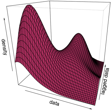
Another important aspect of traffic congestion is that it can be “decomposed” into recurrent and non-recurrent factors. For example, a typical commute time from a western suburb to Chicago’s city center on Mondays is 45 minutes. However, occasionally the travel time is 10 minutes shorter or longer. Figure 4 shows summarized data collected from the sensor located eight miles from the Chicago downtown on I-55 northbound, which is part of a route used by many morning commuters to travel from southwest suburbs to the city. Figure 4(a) shows average speed on the selected road segment for each of the five work days; we can see that there is little variation, on average, from one week day to another with travelers most likely to experience delays between 5 and 10am. However, if we look at the empirical probability distribution of travel speeds between 7 and 8 am on the same road segment on Figure 4(b), we see that distribution is bi-modal. In most cases, the speed is around 20 miles per hour, which corresponds to heavy congestion. The free flow speed on this road segment is around 70 miles per hour. Furthermore, the distribution has a heavy left tail. Thus, on many days the traffic is considerably worse, compared to an “average” day.

(a) Average speed on work days	(b) Empirical density for speed, on work days

Figure 4: Traffic patterns on different days of the week. Left panel (a) shows average speed on work days. Right panel (b) shows empirical density for speed, for five work days of the week. Calculated based on the data collected between 7 and 8am.

Figure 5(a) shows measurements from all non-holiday Wednesdays in 2009. The solid line and band, represent the average speed and 60% confidence interval correspondingly. Each dot is an individual speed measurement that lies outside of 98% confidence interval. Measurements are taken every five minutes, on every Wednesday of 2009; thus, we have roughly 52 measurements for each of the five-minute intervals.

(a) Speed measured on Thursdays	(b) Example of one day speed profile

Figure 5: Recurrent speed profile. Both plots show the speed profile for a segment of interstate highway I-55. Left panel (a) shows the green line, which is the average cross-section speed for each of five minute intervals with 60% confidence interval. The red points are measurements that lie outside of 98% confidence interval. Right panel (b) shows an example of one day speed profile from May 14, 2009 (Thursday).

We see that in many cases traffic patterns are very similar from one day to another. However, there are many days when we see surprises, both good and bad. A good surprise might happen, e.g., when schools are closed due to extremely cold weather. A bad surprise might happen due to non-recurrent traffic conditions, such as an accident or inclement weather.

Figure 5(b) illustrates a typical day’s traffic flow pattern on Chicago’s I-55 highway. This traffic pattern is recurrent, we can see a breakdown in flow speed during the morning peak period, followed by speed recovery. The free flow regimes are usually of little interest to traffic managers.

Figure 6 shows the impact of non-recurrent events. In this case, the traffic speed can significantly deviate from historical averages due to the increased number of vehicles on the road or due to poor road surface conditions.

(a) Chicago Bears football game	(b) Snow weather

Figure 6: Impact of non-recurrent events on traffic flows. Left panel (a) shows traffic flow on a day when New York Giants played at Chicago Bears on Thursday October 10, 2013. Right panel (b) shoes impact of light snow on traffic flow on I-55 near Chicago on December 11, 2013. On both panels average traffic speed is red line and speed on event day is blue line.

Our goal is to build a statistical model to capture the sudden regime changes from free flow to congestion and then the decline in speed to the recovery regime for both recurrent traffic conditions and non-recurrent ones.

As described above, the traffic congestion usually originates at a specific bottlenecks on the network. Therefore, given a bottleneck, our forecast predicts how fast it will propagate on the network. Figure 7, shows that the the spatial-temporal relations in traffic data is non linear.

(a) auto-correlation	(b) cross-correlation

Figure 7: Space-time relation between speed measurements. Left panel (a) shows empirical density estimation for the $(s^{10}_{n},s^{10}_{n-8})$ bivariate random variable, where $s_{n}$ is the speed measured at sensor $10$ at time $n$. Right panel (b) shows empirical density estimation for the $(s^{10}_{n},s^{20}_{n-8})$ bivariate random variable.

We now show how to build a deep learning predictor that can capture the nonlinear nature, as well as spatial-temporal patterns in traffic flows.

3.2 Predictor Selection

Our deep learning model will estimate an input-output map, $x_{t+h}^{t}=\hat{y}_{w,b}(x^{t})$, where $(w,b)$ index weights and parameters and $x^{t}$ is the vector of measurements. Our prior assumption is that to predict traffic at a location we need to use recent measurements from all other sensors on the network. We use previous 12 measurements from each sensor that corresponds to one hour period.

One caveat is that it is computationally prohibitive to use data from every road segment to develop a forecast for a given location and there is some locality in the casual relations between congestion patterns on different road segments. For example, it is unreasonable to assume that a congested arterial in a central business district is related to congestion in a remote suburb, sixty miles away. Thus, it might appear logical to select neighbor road segments as predictors. However, it leads to a large number of unnecessary predictors. For example, congestion in one direction (i.e., towards the business district) does not mean there will be congestion in the opposite direction, which leads to the possibility of using topological neighbors as predictors. The caveat is that by using topological neighbors, it is possible not to include important predictors. For example, when an arterial road is an alternative to a highway, those roads will be strongly related, and will not be topological neighbors.

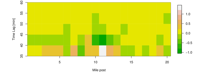
Methods of regularization on the other hand provide the researcher with an automated approach to select predictors. Least angle regression (LARS) is used to fit the $\ell_{1}$ regularized loss function (LASSO) and to find a sparse linear model. Figure 8 shows the sparsity pattern of the resulting coefficient matrix.

Figure 8: Sparsity patterns of the coefficient matrix found by least angle regression (LARS)

Figure 9 shows the magnitude of the coefficients of the linear model for sensor 11. There are 120 predictors used for each of the locations that correspond to 6 lagged measurements from 20 sensors. We see that the largest coefficient is the one that corresponds to the most recent measurement from the sensor itself (white-colored rectangle). We also see that the model does assign the largest values to variables that are close to the modeled variable in time and space. Most of the weight will be on the most recent measurement (lag of 35 minutes). The previous measurement, which corresponds to a lag of 40 minutes, has negative weight. It means that the weighted difference between two consecutive measurements is used as a predictor. Intuitively, it means that the change in speed is the predictor rather than the absolute value of speed. In a time series context, negative weights correspond to cyclic behavior in the data, see Shumway and Stoffer [2010].

Figure 9: Values of coefficients of the fitted linear model for predicting sensor 11.

Another way is to find a sparse neural network model is to apply a dropout operation. Suppose that we have an $\ell_{2}$ objective

$$\operatorname*{argmin}_{w,b}\;\|y-\hat{y}_{w,b}(x)\|_{2}^{2}.$$

Due to the composite nature of the predictor, we can calculate derivative information $\nabla_{w,b}\;l(y,\hat{y}_{w,b}(x))$ using the chain rule via procedure known as backpropagation.

To perform model or variable selection, suppose that we dropout any input dimension in $x$ with probability $p$. This replaces the input by $D\star x$ where $\star$ denotes element-wise products and $D$ is a matrix of $Ber(p)$ random variables. Marginalize over the randomness, we have a new objective

$$(\hat{w},\hat{b})\in\operatorname*{argmin}_{w,b}\;E_{D\sim{\rm Ber}(p)}\left(\|y-\hat{y}_{D\star w,b}(x)\|_{2}^{2}\right),$$

which is equivalent to

$$(\hat{w},\hat{b})\in\operatorname*{argmin}_{w,b}\;\|y-\hat{y}_{w,b}(x)\|_{2}^{2}+p(1-p)\|\Gamma w\|^{2},$$

where $\Gamma=({\rm diag}(X^{\top}X))^{\frac{1}{2}}$ and $X$ is the matrix of observed features. Therefore, the objective function dropout is equivalent to a Bayes ridge regression with a $g$-prior George [2000].

The end model has minimal deviance for a validation data set. We used data from 180 days to fit and test the model, we used the first half of the selected days for training and the remaining half for testing the models.

3.3 Chicago Highway Case Study Results

Having motivated our modeling approach and described general traffic flow patterns, we now evaluate predictive power of sparse linear vector autoregressive (VAR) and deep learning models. Using loop detector data from 21 sensors installed on Chicago’s Interstate highway I-55 measure in the year of 2013. They cover a 13-mile stretch of a highway that connects southwest suburbs to Chicago’s downtown. In our empirical study, we predict traffic flow speed at the location of senor 11, which is in the middle of the 13-mile stretch. It is located right before Cicero Avenue exit from I-55. We treated missing data by doing interpolation on space, i.e. the missing speed measurement $s_{it}$ for sensor $i$ at time $t$ will be amputated using $(s_{i-1t}+s_{i+1t})/2$. Data from days when the entire sensor network was down were excluded from the analysis. We also excluded public holidays and weekend days.

We compare the performance of the deep learning (DL) model with sparse linear vector autoregressive (VAR), combined with several data pre-filtering techniques, namely median filtering with a window size of 8 measurements (M8) and trend filtering with $\lambda=15$ (TF15). We also tested performance of the sparse linear model, identified via regularization. We estimate the percent of variance explained by model, and mean squared error (MSE), which measures average of the deviations between measurements and model predictions. To train both models we selected data for 90 days in 2013. We further selected another 90 days for testing data set. We calculated $R^{2}$ and MSE for both in-sample (IS) data and out-of-sample (OS) data. Those metrics are shown in Table 1.

DLL DLM8L DLM8 DLTF15L DLTF15 VARM8L VARTF15L IS MSE 13.58 7.7 10.62 12.55 12.59 8.47 15 IS $R^{2}$ 0.72 0.83 0.76 0.75 0.75 0.81 0.7 OS MSE 13.9 8.0 9. 5 11.17 12.34 8.78 15.35 OS $R^{2}$ 0.75 0.85 0.82 0.81 0.79 0.83 0.74

Table 1: In sample and out-of-sample metrics for different models. The abbreviations for column headers are as follows: DL = deep learning, VAR = linear model, M8 = media filter preprocessing, TF15 = trend filter preprocessing and L = sparse estimator (lasso). The abbreviations for row headers are as follows: IS = in-sample, MSE = mean squared error and OS = out-of-sample.

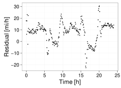
The performance of the model is not uniform throughout the day. Figure 10 shows the absolute values of the residuals (red circles) against the measured data (black line). Highest residuals are observe at when traffic flow regime changes from one to another. On a normal day large errors are observed at around 6am, when regime changes from free flow to congestion and at around 10am, right before it starts to recover back to free flow.

model bears game weather day normal day DLM8L VARM8L

Figure 10: Comparison of the residuals forecasts over time. On all plots black solid line is the measured data (cross-section speed), red dots are absolute values of residuals from our model’s forty minute forecast. First column compares models for data from Thursday October 10, 2013, the day when Chicago Bears team played New York Giants. The game starts at 7pm and lead to an unusual congestion starting at around 4pm. Second column compares models for data from Wednesday December 11, 2013, the day of light snow. The snow leads to heavier congestion during both, the morning and evening rush hours. Third column compares models for data from Monday October 7, 2013. There were no special events, accidents or inclined weather conditions on this day.

Sparse deep learning combined with the median filter pre-processing (DLM8L) shows the best overall performance on the out-of-sample data.

Figure 11 shows performance of both vector auto-regressive and deep learning models for normal day, special event day (Chicago Bears football game) and poor weather day (snow day). We compare our models against the naive constant filter, i.e forecast speed is the same as the current speed. The naive forecast is used by travelers when making route choices before departure. We achieve this by looking at current traffic conditions and assuming those will hold throughout the duration of the planned trip.

Both deep learning (DL) and vector auto-regressive (VAR) models accurately predict the morning rush hour congestion on a normal day. However, the vector auto-regressive model mis-predicts congestion during evening rush hour. At the same time, deep learning model does predict breakdown accurately but miss-estimates the time of recovery. Both deep learning and linear model outperform naive forecasting, when combined with data pre-processing. However, when unfiltered data is used to fit deep learning combined with sparse linear estimator (DLL) model, their predictive power degrades and were out-performed by a naive forecast. Thus, showing the importance of using filtered data to develop forecasts.

model bears game weather day normal day DLM8L VARM8L DLL

Figure 11: Comparison of the forecasts. On all plots black solid line is the measured data (cross-section speed), red dashed line is our model’s forty minute forecast and dashed blue line is naive forecast. Green dashed horizontal line is the speed limit (55 mi/h) and vertical orange line is the morning peak hour (8am). First column compares models for data from Thursday October 10, 2013, the day when Chicago Bears team played New York Giants. The game starts at 7pm and lead to an unusual congestion starting at around 4pm. Second column compares models for data from Wednesday December 11, 2013, the day of light snow. The snow leads to heavier congestion during both, the morning and evening rush hours. Third column compares models for data from Monday October 7, 2013. There were no special events, accidents or inclined weather conditions on this day.

Typically, congestion starts at a bottleneck location and propagates downstream. However, traffic slows down at several locations at the same time during the snow. Thus, for all three models, there is a lag between the forecast and real data for the "weather day" case. We think, that adding a weather forecast as a predictor variable will improve forecasts for traffic caused by snow or rain. The vector autoregressive (VAR) model forecasts lag the data for all three days. Our vector autoregressive model shows surprisingly good performance predicting the normal day traffic, that is comparable to the deep learning model forecast. Deep learning predictor, can produce better predictions for non-recurrent events, as shown for our Bears game and weather day forecasts example.

Another visual way to interpret the results of prediction is via a heat plot. Figure 12 compares the original data and forecasted data. To produce forecast plot we replaced column 11 of the original data (mile post 6) with the forecast for this specific location.

(a) Original Data	(b) Forecast

Figure 12: Heat plot for traffic spreads on Thursday October 10, 2013, the day of the Bears game. Right panel (b) was produced by replacing column 11 (mile post 6) of the measured data with forecast for this location.

From Figure 12 we see that deep learning model properly captures both forward and backward shock wave propagation during morning and evening rush hours.

3.4 Residual Diagnostics

To assess the accuracy of a forecasting model we analyze the residuals, namely the difference between observed value and its forecast $r_{i}=y_{i}-\hat{y}_{i}$. Our goal is to achieve residuals that are uncorrelated with zero mean. In other words, there is no information left in the residuals that can be used to improve the model. Models with the best residuals do not necessarily have the most forecasting power, out of all possible models, but it is an important indicator of whether a model uses all available information in the data.

VARM8
DLM8
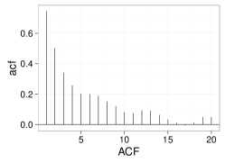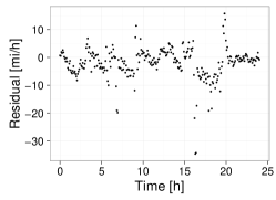
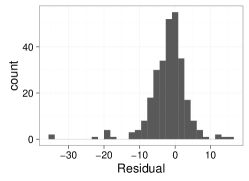
	(a) Time plot	(b) Histogram	(c) Autocorrelations

Figure 13: Residual diagnostics plots for both vector auto-regressive and deep learning models. All plots are for residuals for data from July 29, 2013 (Monday).

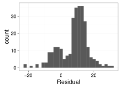
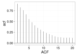
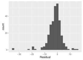
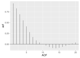
Figure 13 shows that both DLM8 and VARM8 models do not account for all available information, they have autocorrelations in the residuals, and there is a structure in the data, that is not exploited by the models. From the autocorrelations plots we can see that deep-learning model residuals are less correlated. Time plots show that deep learning residuals have less patterns and more uniform variance, compared to a VAR model. The histograms suggest that VAR residuals do not follow a normal distribution and DL do. Both of the models are biased, with mean residual for DL model being -2 and mean residual for VAR model being -7.

Results of formal residual tests are shown in Table 2.

Test	NULL	VARM8	DLM8
Breusch-Godfrey	no autocorrelations	4.27 (0.005)	1.8 (0.15)
Box-Pierce	no autocorrelations	995.77 (0)	323.64 (0)
Breusch-Pagan	homoscedasticity	6.62 (0.037)	4.08 (0.13)
Lee-White-Granger	linearity in mean	2.1 (0.13)	0.16 (0.85)
Dickey-Fuller	non-stationary	-3.0154 (0.15)	-3.39 (0.05)

Table 2: Results of the formal statistical tests for for autocorrelation, non-linearity, homoscedasticity and stationarity in model residuals. The table shows value of the corresponding test statistic and p-value (in parentheses)

A classical Box-Ljung test Box and Pierce [1970] for autocorrelation shows that both models produce autocorrelated residuals. The $Q$-statistic, which is an aggregate measure of autocorrelation, is much higher for VAR model. However, as pointed out in previous neural networks applications to traffic analysis Vlahogianni and Karlaftis [2013], statistical tests based on Lagrange multiplier (LM) are more appropriate for the residual analysis. Medeiros et al. [2006], for example, notes that the asymptotic distribution of the test statistics in Box-Ljung test is unknown when a neural network model is used. Thus, we use a more appropriate LM-based Breusch-Godfrey test Hayashi [2000] to detect the autocorrelations, Breusch-Pagan test for homoscedasticity and Lee-White-Granger Lee et al. [1993] test for linearity in “mean” in the data. The LM-based tests suggest that the residuals from the deep learning model are less correlated, and more homoscedastic when compared to VAR model residuals. Though, we have to accept the linearity Null hypothesis for both models, according to Lee-White-Granger, the $p$ value is much higher for the deep learning model. Another important finding is that the residuals are stationary for the DL model and are non-stationary for the VAR model. The formal Augmented Dickey-Fuller (ADF) test produced $p$-value of 0.06 for DL model and 0.15 for VAR model, with alternative hypothesis being that data is stationary. Stationary residuals mean that the model correctly captures all of the trends in the data.

Kolmogorov-Smirnov test shows that neither DL nor VAR model residuals are normally distributed. On the other hand, the residuals from DL model are less biased and are less correlated.

3.5 Comparison to a single layer neural network

Finally, deep learning is compared with a simple neural network model with one hidden layer. We used median filtering with a window size of 8 measurement (M8) as a preprocessing technique and predictors are pre-chosen using a sparse linear estimator. The in sample $R^{2}$ is 0.79 and MSE is 9.14. The out of sample metrics are 0.82 and 9.12.

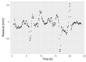
(a) Time plot	(b) Histogram	(c) Autocorrelations

Figure 14: Residual diagnostics plots for neural network with one hidden layer. All plots are for residuals for data from July 29, 2013 (Monday).

The performance of the neural network model with one hidden layer is slightly worse than the one of the best linear model (VARM8L), the MSE is 4% higher and 14% higher when compared to the deep learning model (DLM8L). As shown in Figure 14, there is excess correlation structure left in the residuals, when compared to DLM8L. The model bias is comparable to the deep learning model and equals to -2.1. A one-layer network model is less efficient and has less predictive power when compared to the deep learning network for traffic data.

4 Discussion

The main contribution of this paper is development of an innovative deep learning architecture to predict traffic flows. The architecture combines a linear model that is fitted using $\ell_{1}$ regularization and a sequence of $\tanh$ layers. The first layer identifies spatio-temporal relations among predictors and other layers model nonlinear relations. The improvements in our understanding of short-term traffic forecasts from deep learning are two-fold. First, we demonstrate that deep learning provides a significant improvement over linear models. Second, there are also other types of networks that demonstrated superior performance for time series data. For example, the recurrent neural network (RNN) is a class of network where connections between units can form a directed cycle. This creates an internal state that allows to memorize previous data. Another class of networks that are capable of motorizing previous data are the long short term memory (LSTM) network, developed in Hochreiter and Schmidhuber [1997]. It is an artificial neural network structure that addresses a problem of the vanishing gradient problem. In a sense, it allows for longer memory and it works even when there are long delays. It can also handle signals that have periodic components of different frequencies. Long short term memory and recurrent neural networks outperformed other methods in numerous applications, such as language learning Gers et al. [2001] and connected handwriting recognition Graves and Schmidhuber [2009].

We empirically observed from data that recent observations of traffic conditions (i.e. within last 40 minutes) are stronger predictors rather than historical values, i.e. measurements from 24 hours ago. In other words, future traffic conditions are more similar to current ones as compared to those from previous days. Thus, it allowed us to develop a powerful model by using recent observations as model features.

One of the drawbacks of deep learning models is low explanatory power. In a recent review of short term forecasting techniques Vlahogianni et al. [2014], model interpretability is mentioned as one of the barriers in adapting more sophisticated machine learning models in practice. The idea of a deep learning model is to develop representations of the original predictor vector so that transformed data can be used for linear regression. There is a large volume of literature on studying representations for different domain specific models. Perhaps, the more advanced research on that topic was done for Natural Language Processing problems Turian et al. [2010], Luong et al. [2013]. One example of such representations are word embeddings, which are vectors associated with each word that contain latent features of the word and capture its syntactic and semantic properties. For example, Miklov and Zweig Mikolov et al. [2013] show that if we calculate induced vector representation, “King - Man + Woman” on vector representation of the corresponding words, we get a vector very close to “Queen.” In the context of traffic predictions, relating the representations of input vectors to the fundamental properties of traffic flow is an interesting and challenging problem which needs to be studied further.

References

- Abadi et al. [2016] Martın Abadi, Ashish Agarwal, Paul Barham, Eugene Brevdo, Zhifeng Chen, Craig Citro, Greg S Corrado, Andy Davis, Jeffrey Dean, Matthieu Devin, et al. Tensorflow: Large-scale machine learning on heterogeneous distributed systems. arXiv preprint arXiv:1603.04467, 2016.
- Anacleto et al. [2013] Osvaldo Anacleto, Catriona Queen, and Casper J Albers. Multivariate forecasting of road traffic flows in the presence of heteroscedasticity and measurement errors. Journal of the Royal Statistical Society: Series C (Applied Statistics), 62(2):251–270, 2013.
- Ban et al. [2011] Xuegang Jeff Ban, Peng Hao, and Zhanbo Sun. Real time queue length estimation for signalized intersections using travel times from mobile sensors. Transportation Research Part C: Emerging Technologies, 19(6):1133–1156, 2011.
- Bastien et al. [2012] Frédéric Bastien, Pascal Lamblin, Razvan Pascanu, James Bergstra, Ian J. Goodfellow, Arnaud Bergeron, Nicolas Bouchard, and Yoshua Bengio. Theano: new features and speed improvements. Deep Learning and Unsupervised Feature Learning NIPS 2012 Workshop, 2012.
- Bishop [1995] Christopher M Bishop. Neural networks for pattern recognition. Oxford university press, 1995.
- Blandin et al. [2012] Sébastien Blandin, Adrien Couque, Alexandre Bayen, and Daniel Work. On sequential data assimilation for scalar macroscopic traffic flow models. Physica D: Nonlinear Phenomena, 241(17):1421–1440, 2012.
- Box and Pierce [1970] George EP Box and David A Pierce. Distribution of residual autocorrelations in autoregressive-integrated moving average time series models. Journal of the American statistical Association, 65(332):1509–1526, 1970.
- Breiman [2003] Leo Breiman. Statistical modeling: The two cultures. Quality control and applied statistics, 48(1):81–82, 2003.
- Breiman et al. [1984] Leo Breiman, Jerome Friedman, Charles J Stone, and Richard A Olshen. Classification and regression trees. CRC press, 1984.
- Çetiner et al. [2010] B Gültekin Çetiner, Murat Sari, and Oğuz Borat. A neural network based trafficflow prediction model. Mathematical and Computational Applications, 15(2):269–278, 2010.
- Chen and Grant-Muller [2001] Haibo Chen and Susan Grant-Muller. Use of sequential learning for short-term traffic flow forecasting. Transportation Research Part C: Emerging Technologies, 9(5):319–336, 2001.
- Chiou et al. [2014] Yu-Chiun Chiou, Lawrence W Lan, and Chun-Ming Tseng. A novel method to predict traffic features based on rolling self-structured traffic patterns. Journal of Intelligent Transportation Systems, 18(4):352–366, 2014.
- Dellaportas et al. [2012] Petros Dellaportas, Jonathan J Forster, and Ioannis Ntzoufras. Joint specification of model space and parameter space prior distributions. Statistical Science, 27(2):232–246, 2012.
- Diaconis and Shahshahani [1984] Persi Diaconis and Mehrdad Shahshahani. On nonlinear functions of linear combinations. SIAM Journal on Scientific and Statistical Computing, 5(1):175–191, 1984.
- Friedman and Tukey [1974] J. H. Friedman and J. W. Tukey. A projection pursuit algorithm for exploratory data analysis. IEEE Transactions on Computers, C-23(9):881–890, Sept 1974. ISSN 0018-9340. doi: 10.1109/T-C.1974.224051.
- George [2000] Edward I George. The variable selection problem. Journal of the American Statistical Association, 95(452):1304–1308, 2000.
- Gers et al. [2001] Felix Gers, Jürgen Schmidhuber, et al. LSTM recurrent networks learn simple context-free and context-sensitive languages. Neural Networks, IEEE Transactions on, 12(6):1333–1340, 2001.
- Graves and Schmidhuber [2009] Alex Graves and Jürgen Schmidhuber. Offline handwriting recognition with multidimensional recurrent neural networks. In Advances in Neural Information Processing Systems, pages 545–552, 2009.
- Hayashi [2000] Fumio Hayashi. Econometrics. 2000. Princeton University Press. Section, 1:60–69, 2000.
- Haykin [2004] Simon Haykin. A comprehensive foundation. Neural Networks, 2(2004), 2004.
- Helmbold and Long [2015] David P Helmbold and Philip M Long. On the inductive bias of dropout. Journal of Machine Learning Research, 16:3403–3454, 2015.
- Hinton and Salakhutdinov [2006] Geoffrey E Hinton and Ruslan R Salakhutdinov. Reducing the dimensionality of data with neural networks. Science, 313(5786):504–507, 2006.
- Hochreiter and Schmidhuber [1997] Sepp Hochreiter and Jürgen Schmidhuber. Long short-term memory. Neural computation, 9(8):1735–1780, 1997.
- Horvitz et al. [2012] Eric J Horvitz, Johnson Apacible, Raman Sarin, and Lin Liao. Prediction, expectation, and surprise: Methods, designs, and study of a deployed traffic forecasting service. arXiv preprint arXiv:1207.1352, 2012.
- Kamarianakis et al. [2012a] Yiannis Kamarianakis, Wei Shen, and Laura Wynter. Real-time road traffic forecasting using regime-switching space-time models and adaptive LASSO. Applied stochastic models in business and industry, 28(4):297–315, 2012a.
- Kamarianakis et al. [2012b] Yiannis Kamarianakis, Wei Shen, and Laura Wynter. Real-time road traffic forecasting using regime-switching space-time models and adaptive LASSO. Applied Stochastic Models in Business and Industry, 28(4):297–315, July 2012b. ISSN 1526-4025. doi: 10.1002/asmb.1937. URL http://onlinelibrary.wiley.com/doi/10.1002/asmb.1937/abstract.
- Karlaftis and Vlahogianni [2011] MG Karlaftis and EI Vlahogianni. Statistical methods versus neural networks in transportation research: differences, similarities and some insights. Transportation Research Part C: Emerging Technologies, 19(3):387–399, 2011.
- Kim et al. [2007] S. J. Kim, K. Koh, M. Lustig, S. Boyd, and D. Gorinevsky. An Interior-Point Method for Large-Scale -Regularized Least Squares. IEEE Journal of Selected Topics in Signal Processing, 1(4):606–617, December 2007. ISSN 1932-4553. doi: 10.1109/JSTSP.2007.910971.
- Kim et al. [2009] Seung-Jean Kim, Kwangmoo Koh, Stephen Boyd, and Dimitry Gorinevsky. trend filtering. SIAM review, 51(2):339–360, 2009.
- Kolmogorov [1956] AN Kolmogorov. On the representation of continuous functions of several variables as superpositions of functions of smaller number of variables. In Soviet. Math. Dokl, volume 108, pages 179–182, 1956.
- Lee et al. [1993] Tae-Hwy Lee, Halbert White, and Clive WJ Granger. Testing for neglected nonlinearity in time series models: A comparison of neural network methods and alternative tests. Journal of Econometrics, 56(3):269–290, 1993.
- Luong et al. [2013] Thang Luong, Richard Socher, and Christopher D Manning. Better word representations with recursive neural networks for morphology. In CoNLL, pages 104–113, 2013.
- Lv et al. [2015] Yisheng Lv, Yanjie Duan, Wenwen Kang, Zhengxi Li, and Fei-Yue Wang. Traffic flow prediction with big data: A deep learning approach. Intelligent Transportation Systems, IEEE Transactions on, 16(2):865–873, 2015.
- Ma et al. [2015] Xiaolei Ma, Zhimin Tao, Yinhai Wang, Haiyang Yu, and Yunpeng Wang. Long short-term memory neural network for traffic speed prediction using remote microwave sensor data. Transportation Research Part C: Emerging Technologies, 54:187–197, 2015.
- Medeiros et al. [2006] Marcelo C. Medeiros, Timo Teräsvirta, and Gianluigi Rech. Building neural network models for time series: a statistical approach. Journal of Forecasting, 25(1):49–75, 2006. ISSN 1099-131X. doi: 10.1002/for.974. URL http://dx.doi.org/10.1002/for.974.
- Microsoft Research [2016] Microsoft Research. Predictive analytics for traffic, 2016. URL {http://research.microsoft.com/en-us/projects/clearflow/}. [online at http://research.microsoft.com/en-us/projects/clearflow/; accessed 14-February-2016].
- Mikolov et al. [2013] Tomas Mikolov, Wen-tau Yih, and Geoffrey Zweig. Linguistic regularities in continuous space word representations. In HLT-NAACL, volume 13, pages 746–751, 2013.
- Muralidharan and Horowitz [2009] Ajith Muralidharan and Roberto Horowitz. Imputation of ramp flow data for freeway traffic simulation. Transportation Research Record: Journal of the Transportation Research Board, (2099):58–64, 2009.
- Nicholson et al. [2014] W Nicholson, D Matteson, and Jacob Bien. Structured regularization for large vector autoregressions. Cornell University, 2014.
- Oswald et al. [2000] R Keith Oswald, William T Scherer, and Brian L Smith. Traffic flow forecasting using approximate nearest neighbor nonparametric regression. Final project of ITS Center project: Traffic forecasting: non-parametric regressions, 2000.
- Pachitariu and Sahani [2013] Marius Pachitariu and Maneesh Sahani. Regularization and nonlinearities for neural language models: when are they needed? arXiv preprint arXiv:1301.5650, 2013.
- Polson and Sokolov [2014] Nicholas Polson and Vadim Sokolov. Bayesian particle tracking of traffic flows. arXiv preprint arXiv:1411.5076, 2014.
- Polson and Sokolov [2015] Nicholas Polson and Vadim Sokolov. Bayesian analysis of traffic flow on interstate i-55: The LWR model. The Annals of Applied Statistics, 9(4):1864–1888, 2015.
- Polson and Scott [2015] Nicholas G Polson and James G Scott. Mixtures, envelopes and hierarchical duality. Journal of the Royal Statistical Society: Series B (Statistical Methodology), 2015.
- Polson and Scott [2011] Nicholas G Polson and Steven L Scott. Data augmentation for support vector machines. Bayesian Analysis, 6(1):1–23, 2011.
- Qiao et al. [2001] Fengxiang Qiao, Hai Yang, and William HK Lam. Intelligent simulation and prediction of traffic flow dispersion. Transportation Research Part B: Methodological, 35(9):843–863, 2001.
- Quek et al. [2006] Chai Quek, M. Pasquier, and B.B.S. Lim. POP-TRAFFIC: a novel fuzzy neural approach to road traffic analysis and prediction. IEEE Transactions on Intelligent Transportation Systems, 7(2):133–146, June 2006. ISSN 1524-9050. doi: 10.1109/TITS.2006.874712.
- Ramdas and Tibshirani [2015] Aaditya Ramdas and Ryan J Tibshirani. Fast and flexible admm algorithms for trend filtering. Journal of Computational and Graphical Statistics, (just-accepted), 2015.
- Ramezani and Geroliminis [2015] Mohsen Ramezani and Nikolas Geroliminis. Queue profile estimation in congested urban networks with probe data. Computer-Aided Civil and Infrastructure Engineering, 30(6):414–432, 2015.
- Rice and van Zwet [2004] J. Rice and E. van Zwet. A simple and effective method for predicting travel times on freeways. IEEE Transactions on Intelligent Transportation Systems, 5(3):200–207, September 2004. ISSN 1524-9050. doi: 10.1109/TITS.2004.833765.
- Ripley [1996] Brian D. Ripley. Pattern recognition and neural networks. Cambridge university press, 1996.
- Rudin et al. [1992] Leonid I Rudin, Stanley Osher, and Emad Fatemi. Nonlinear total variation based noise removal algorithms. Physica D: Nonlinear Phenomena, 60(1):259–268, 1992.
- Shumway and Stoffer [2010] Robert H Shumway and David S Stoffer. Time series analysis and its applications: with R examples. Springer Science & Business Media, 2010.
- Smith and Demetsky [1997] Brian L Smith and Michael J Demetsky. Traffic flow forecasting: comparison of modeling approaches. Journal of transportation engineering, 123(4):261–266, 1997.
- Srivastava et al. [2014] Nitish Srivastava, Geoffrey Hinton, Alex Krizhevsky, Ilya Sutskever, and Ruslan Salakhutdinov. Dropout: A simple way to prevent neural networks from overfitting. The Journal of Machine Learning Research, 15(1):1929–1958, 2014.
- Strub and Bayen [2006] Issam Strub and Alexandre Bayen. Weak formulation of boundary conditions for scalar conservation laws: An application to highway traffic modelling. International Journal of Robust and Nonlinear Control, 16(16):733–748, 2006.
- Sun et al. [2006] Shiliang Sun, Changshui Zhang, and Guoqiang Yu. A bayesian network approach to traffic flow forecasting. IEEE Transactions on Intelligent Transportation Systems, 7(1):124–132, March 2006. ISSN 1524-9050. doi: 10.1109/TITS.2006.869623.
- Tan et al. [2009] Man-Chun Tan, S.C. Wong, Jian-Min Xu, Zhan-Rong Guan, and Peng Zhang. An Aggregation Approach to Short-Term Traffic Flow Prediction. IEEE Transactions on Intelligent Transportation Systems, 10(1):60–69, March 2009. ISSN 1524-9050. doi: 10.1109/TITS.2008.2011693.
- Tebaldi and West [1998] Claudia Tebaldi and Mike West. Bayesian inference on network traffic using link count data. Journal of the American Statistical Association, 93(442):557–573, 1998.
- Tibshirani and Taylor [2011] Ryan J. Tibshirani and Jonathan Taylor. The solution path of the generalized lasso. Ann. Statist., 39(3):1335–1371, 06 2011. doi: 10.1214/11-AOS878. URL http://dx.doi.org/10.1214/11-AOS878.
- TransNet [2016] TransNet. I-15 express lanes corridor, 2016. URL {http://keepsandiegomoving.com/i-15-corridor/i-15-intro.aspx}. [online at http://keepsandiegomoving.com/i-15-corridor/i-15-intro.aspx; accessed 14-February-2016].
- Turian et al. [2010] Joseph Turian, Lev Ratinov, and Yoshua Bengio. Word representations: a simple and general method for semi-supervised learning. In Proceedings of the 48th annual meeting of the association for computational linguistics, pages 384–394. Association for Computational Linguistics, 2010.
- Van Der Voort et al. [1996] Mascha Van Der Voort, Mark Dougherty, and Susan Watson. Combining kohonen maps with arima time series models to forecast traffic flow. Transportation Research Part C: Emerging Technologies, 4(5):307–318, 1996.
- van Hinsbergen et al. [2009] CP IJ van Hinsbergen, JWC Van Lint, and HJ Van Zuylen. Bayesian committee of neural networks to predict travel times with confidence intervals. Transportation Research Part C: Emerging Technologies, 17(5):498–509, 2009.
- Van Lint [2008] J.W.C. Van Lint. Online Learning Solutions for Freeway Travel Time Prediction. IEEE Transactions on Intelligent Transportation Systems, 9(1):38–47, March 2008. ISSN 1524-9050. doi: 10.1109/TITS.2008.915649.
- Van Lint et al. [2005] JWC Van Lint, SP Hoogendoorn, and Henk J van Zuylen. Accurate freeway travel time prediction with state-space neural networks under missing data. Transportation Research Part C: Emerging Technologies, 13(5):347–369, 2005.
- Vlahogianni and Karlaftis [2013] Eleni Vlahogianni and Matthew Karlaftis. Testing and comparing neural network and statistical approaches for predicting transportation time series. Transportation Research Record: Journal of the Transportation Research Board, (2399):9–22, 2013.
- Vlahogianni et al. [2005] Eleni I Vlahogianni, Matthew G Karlaftis, and John C Golias. Optimized and meta-optimized neural networks for short-term traffic flow prediction: a genetic approach. Transportation Research Part C: Emerging Technologies, 13(3):211–234, 2005.
- Vlahogianni et al. [2014] Eleni I Vlahogianni, Matthew G Karlaftis, and John C Golias. Short-term traffic forecasting: Where we are and where we’re going. Transportation Research Part C: Emerging Technologies, 43:3–19, 2014.
- Wager et al. [2013] Stefan Wager, Sida Wang, and Percy S Liang. Dropout Training as Adaptive Regularization. In C. J. C. Burges, L. Bottou, M. Welling, Z. Ghahramani, and K. Q. Weinberger, editors, Advances in Neural Information Processing Systems 26, pages 351–359. Curran Associates, Inc., 2013. URL http://papers.nips.cc/paper/4882-dropout-training-as-adaptive-regularization.pdf.
- Westgate et al. [2013] Bradford S Westgate, Dawn B Woodard, David S on, Shane G Henderson, et al. Travel time estimation for ambulances using bayesian data augmentation. The Annals of Applied Statistics, 7(2):1139–1161, 2013.
- Work et al. [2010] Daniel B Work, Sébastien Blandin, Olli-Pekka Tossavainen, Benedetto Piccoli, and Alexandre M Bayen. A traffic model for velocity data assimilation. Applied Mathematics Research eXpress, 2010(1):1–35, 2010.
- Wu et al. [2004] Chun-Hsin Wu, Jan-Ming Ho, and D.T. Lee. Travel-time prediction with support vector regression. IEEE Transactions on Intelligent Transportation Systems, 5(4):276–281, December 2004. ISSN 1524-9050. doi: 10.1109/TITS.2004.837813.
- Zheng et al. [2006] Weizhong Zheng, Der-Horng Lee, and Qixin Shi. Short-term freeway traffic flow prediction: Bayesian combined neural network approach. Journal of transportation engineering, 132(2):114–121, 2006.