Electrical conductivity of the lowermost mantle explains absorption of core torsional waves at the equator

Abstract

Torsional Alfvén waves propagating in the Earth’s core have been inferred by inversion techniques applied to geomagnetic models. They appear to propagate across the core but vanish at the equator, exchanging angular momentum between core and mantle. Assuming axial symmetry, we find that an electrically conducting layer at the bottom of the mantle can lead to total absorption of torsional waves that reach the equator. We show that the reflection coefficient depends on $G\tilde{B}_{r}$, where $\tilde{B}_{r}$ is the strength of the radial magnetic field at the equator, and $G$ the conductance of the lower mantle there. With $\tilde{B}_{r}=7\times 10^{-4}$ T., torsional waves are completely absorbed when they hit the equator if $G\simeq 1.3\times 10^{8}$ S. For larger or smaller $G$, reflection occurs. As $G$ is increased above this critical value, there is less attenuation and more angular momentum exchange. Our finding dissociates efficient core-mantle coupling from strong ohmic dissipation in the mantle.

1 Introduction

Geostrophic motions propagating outward from the cylindrical surface tangent to the inner core and vanishing, 3 to 4 years later, upon their arrival near the outer core equator have been detected by Gillet et al. [2010]. In order to estimate the magnetic field intensity in the Earth’s core interior, they relied on a model of one-dimensional torsional Alfvén waves propagating in a spherical shell filled by a perfectly conducting and inviscid fluid [Braginsky, 1970]. They found that the model reproduces well the propagation pattern of the geostrophic motions in a certain range of values of $G\tilde{B}_{r}^{2}$, where $G$ is the conductance of the mantle and $\tilde{B}_{r}$ is the rms value of the radial field at the core-mantle boundary. Assuming that $\tilde{B}_{r}$ is $7\times 10^{-4}$ T., they estimated the conductance to be between $6\times 10^{7}$ S. and $2.8\times 10^{8}$ S. They interpreted their results in terms of magnetic friction at the core-mantle boundary damping the torsional waves. In this process, angular momentum is exchanged between core and mantle, contributing to the length-of-day variations.

Gillet et al. [2015] examined torsional wave propagation in the Earth’s core over a longer time interval (1940-2010) and confirmed that the waves repeatedly travel from the cylinder circumscribing the inner core to the outer core equator, where they disappear. Magnetic fields originating in the core are possibly delayed across the electrically conducting mantle but Gillet et al. [2015] also remarked that the phase retardation $\tau$ between changes in the length-of-day and core angular momentum series calculated from magnetic data is very small, namely less than half a year (Holme and De Viron [2013] argued for an even smaller phase lag $\tau\leq 0.2$ yr). Assuming spherical symmetry and that the conductivity varies smoothly with radius, Jault [2015] inferred from this constraint on the low-frequency electromagnetic delay time of the mantle an upper limit on the mantle conductivity that corresponds to $G\leq 3\times 10^{7}$ S. This calculation leaves aside a possible thin layer of high conductance at the bottom of the mantle [Buffett and Christensen, 2007] that may consist of post-perovskite [Ohta et al., 2008] or iron-rich (Mg,Fe)O assemblage [Wicks et al., 2010].

Investigating torsional wave models from a theoretical standpoint, Schaeffer et al. [2012] remarked that while the values of the viscosity and the magnetic diffusivity in the core interior are unimportant, their ratio $Pm$ (the magnetic Prandtl number) determines the reflection at the equator. There, the core-mantle boundary can be approximated as a plane parallel to the rotation axis. Using a one-dimensional Alfvén wave theory, Schaeffer et al. [2012] computed a reflection coefficient $R$, defined as the ratio of the outgoing fluid velocity amplitude over the incoming one:

$$R=\frac{1-\sqrt{Pm}}{1+\sqrt{Pm}},$$ (1)

for an insulating wall. With two-dimensional numerical simulations, they showed that the one-dimensional plane wave theory is a useful guide for torsional waves in the spherical geometry of the Earth’s core, although there are some differences. Hence, they argued that in the case of most geodynamo simulations, which have been performed with $Pm\sim 1$, there is no significant reflection of torsional Alfvén waves. However, this effect can not explain the propagation pattern of geostrophic motions inferred by Gillet et al. [2010] as $Pm$ is about $10^{-6}$ in the Earth’s core. Here, we show that the value of $Pm$ becomes unimportant in the presence of an electrically conducting layer at the bottom of the mantle. The reflection coefficient at the equator depends on $Q+\sqrt{Pm}$, where the dimensionless number $Q$ varies linearly with the conductance $G$ of the mantle. It is likely that $\sqrt{Pm}\ll Q$ in the geophysical situation. We can thus interpret the propagation pattern of geostrophic motions in terms of poor reflection on the conducting mantle at the equator instead of magnetic damping distributed throughout the core. Our estimate of the conductance $G$ that corresponds to poor reflection is about the same as the preferred value of Gillet et al. [2010].

The paper is organized as follows. We first combine, in section 2, a theoretical study in planar geometry – where a vertical wall models the core-mantle boundary next to the equator – with a discussion of axisymmetric numerical simulations in spherical geometry. We find that the reflection coefficient is correctly estimated from the study of a one-dimensional Alfvén wave hitting a conducting wall. Section 3 is devoted to a discussion of the geophysical case. Energy dissipation in the equatorial region is a non monotonous function of the mantle electrical conductivity. Accordingly, torsional waves may propagate almost unhindered by magnetic friction in the core volume and yet be almost fully absorbed at the equator.

2 Reflection of torsional waves at the outer core equator

2.1 Plane wave theory

Using a plane wave approach, we can derive analytically the reflection of one-dimensional Alfvén waves propagating in the half-space $0<x$ on a conducting wall at $x=0$ (see the detailed calculation in Appendix A):

$$R\simeq\frac{1-Q-\sqrt{Pm}}{1+Q+\sqrt{Pm}}\,,$$ (2)

with

$$Q=\sqrt{\frac{\mu_{0}}{\rho}}\,G\,B\,,\qquad Pm=\frac{\nu}{\eta}\,,$$ (3)

$B$ the magnetic field perpendicular to the wall, $\rho$ the fluid density, $\nu$ its kinematic viscosity, $\eta$ its magnetic diffusivity, $\mu_{0}$ the magnetic permeability of free space and $G$ the conductance of the solid region ($-\delta\leq x\leq 0$):

$$G=\int_{-\delta}^{0}\sigma(x)\mathrm{d}x\,.$$ (4)

To obtain (2), we have assumed that the electromagnetic skin depth in the solid domain is larger than the conducting layer thickness (low-frequency approximation), in which case $R$ is a real number. In the limit of small $Pm$, which is relevant for liquid metals, no reflection occurs when $Q\simeq 1$.

Figure 1: Reflected energy of a one-dimensional Alfvén wave as a function of the conductance of the wall. We set $Pm=10^{-6}$ and $V_{A}=6.24\times 10^{-3}$ m/s corresponding to $B=7\times 10^{-4}$ T with $\rho=10^{4}$ kg/m³, values which are representative of the Earth’s core.

Plotting $R$ as a function of $G$ for Earth-like values of $B=7\times 10^{-4}$ T, $\rho=10^{4}$ kg/m³ and $Pm=10^{-6}$, we find that the reflected energy is close to zero for a solid conducting layer next to the fluid with a conductance of $G\simeq 10^{8}$ S., as seen in figure 1.

The parameters $Pm$ and $Q$ determine where energy dissipation takes place (see Appendix B). Whatever the value of $Pm$, there is always equal dissipation of magnetic and kinetic energy within the Hartmann boundary layer. The ratio of dissipation in the solid wall and in this fluid layer scales as $Q/2\sqrt{Pm}$ although the dissipation in the wall,

$${Q(1+R)^{2}}=\frac{4Q}{(1+Q+\sqrt{Pm})^{2}}\,,$$ (5)

vanishes in the limit $Q\rightarrow\infty$. In this limit, which corresponds to $R=-1$, there is maximal exchange of momentum between the fluid and the solid at each reflection but no dissipation. The value of $Q/\sqrt{Pm}$ establishes which of the Hartmann layer or the conducting solid wall plays the main part in the reflection mechanism (see also equation (2)).

2.2 Simulations in spherical geometry

We have performed numerical simulations of the propagation of a torsional Alfvén wave pulse in a spherical shell of inner radius $r_{i}=0.35$ and outer radius $r_{o}=1$ permeated by an axially symmetric magnetic field $\mathbf{B}$, which is the gradient of a potential. The simulations are of the same type as the ones done by Schaeffer et al. [2012], except for the addition of a conducting solid layer of thickness $\delta$ surrounding the fluid. The XSHELLS code is used to time-step the linearized Navier-Stokes equation coupled to the linearized induction equation:

$$\partial_{t}\mathbf{u}+2\mathbf{\Omega}\times\mathbf{u} = -\nabla p^{*}+\nu\nabla^{2}\mathbf{u}+\frac{1}{\rho\mu_{0}}(\nabla\times\mathbf{b})\times\mathbf{B},$$ (6)

$$\partial_{t}\mathbf{b} = \nabla\times(\mathbf{u}\times\mathbf{B}-\eta\nabla\times\mathbf{b}),$$ (7)

where $\eta=(\mu_{0}\sigma)^{-1}$ is the magnetic diffusivity. The electrical conductivity $\sigma$ is uniform in the fluid and jumps to another uniform value $\sigma_{m}$ in the solid outer shell.

The imposed magnetic field is an external axial quadrupole $\mathbf{B}=B\,(2z\mathbf{e_{z}}-s\mathbf{e_{s}})$. In this context, we define the Alfvén velocity as $V_{A}=B/\sqrt{\mu_{0}\rho}$. We hold the following parameters fixed across all simulations: the magnetic Prandtl number $Pm=10^{-3}$, the Ekman number $E=\nu/r_{0}^{2}\Omega=10^{-10}$, the Lehnert number $Le=V_{A}/\Omega r_{o}=9.46\times 10^{-4}$. This implies a Lundquist number $V_{A}r_{0}/\eta\simeq 10^{4}$. No-slip boundary conditions are used at $r=r_{o}$ while free-slip are used at $r=r_{i}$ to avoid a very thin Ekman layer there. The inner-core is insulating, while a solid conducting layer of thickness $\delta=0.025\,r_{0}$ is included at the bottom of the mantle. In this region, we time-step the induction equation (7) with $\mathbf{u}=0$. The XSHELLS code uses the spherical harmonic transform of the SHTns library [Schaeffer, 2013] in the angular coordinates and finite differences in the radial direction. The finite difference scheme handles conductivity jumps as detailed by Cabanes et al. [2014]. A semi-implicit time-stepping scheme is used with diffusive terms (for both the momentum and the induction equations) handled by a Crank-Nicolson scheme, while all other terms are treated explicitly by a second order Adams-Bashforth scheme. In order to fully resolve the very thin boundary layers (both viscous and magnetic) that occur near $r=r_{0}$, we need $N_{r}=5000$ radial shells. The spherical harmonic expansion, which is restricted here to axisymmetric functions, is truncated after harmonic degree $\ell_{max}=500$.

We have chosen the following initial condition which corresponds to an outgoing pulse (propagating towards the equator):

$$\mathbf{b}=\mathbf{u}=s\,\exp\left(-\frac{(s-s_{0})^{2}}{d^{2}}\right)\mathbf{e_{\phi}},$$ (8)

with $s_{0}=(r_{0}+r_{i})/2$ and either $d=0.02$ or $d=0.071$.

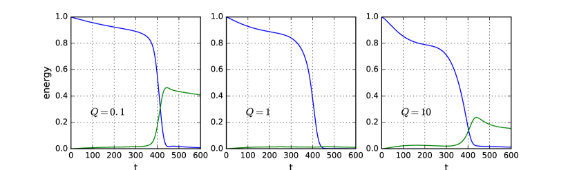
Figure 2: Evolution of the energy of the incoming (blue) and reflected (green) pulses as a function of time in spherical shell simulations for $Pm=10^{-3}$, $E=10^{-10}$ and $S\simeq 10^{4}$. Reflection occurs at about $t=400$. There is no reflected pulse when the conductivity of the solid layer is such that $Q=1$.

We note $\eta_{m}=(\mu_{0}\sigma_{m})^{-1}$ the magnetic diffusivity in the solid conducting layer. Twelve values of $\eta_{m}$, all larger than the magnetic diffusivity $\eta$ of the fluid, have been used, spanning five orders of magnitude. We note

$$Q=\sqrt{\frac{\mu_{0}}{\rho}}GB_{r}|_{r=r_{o},\theta=\pi/2},\qquad\mathrm{with}\qquad G=\int_{r_{o}}^{r_{o}+\delta}\sigma_{m}(r)\mathrm{d}r\,.$$ (9)

Figure 2 shows the evolution of the energy of the incoming and reflected wave fields for three of these simulations. From this time history, we compute $|R|^{2}$, related to the reflection coefficient $R$. It conforms with the theoretical prediction (2) obtained from the study of one-dimensional Alfvén waves hitting a wall at $S\to\infty$. The agreement is especially good for $Q\sim 1$ as shown by figure 3.

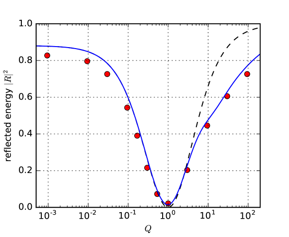
Figure 3: Reflection of torsional Alfvén waves in spherical shell numerical simulations ($Pm=10^{-3}$, $E=10^{-10}$, $S\sim 10^{4}$). Red dots are the measured reflected energy ratio $R^{2}$ in the simulations. The blue line is the exact plane-wave theory (with $R$ depending on the wavelength), while the black dashed line is the thin layer approximation (which does not depend on the wavelength).

3 Discussion

In our study, we have used a simple magnetic field, with almost uniform strength and for parameters that have not been reached previously $E=\nu/r_{0}^{2}\Omega=10^{-10}$ and $Pm=10^{-3}$. In addition, we have considered a uniform conductivity in the lowermost mantle together with a magnetic field independent of the longitude.

In this framework, attenuation of the torsional Alfvén waves that reach the equator is maximized in the vicinity of $Q=1$, which makes this value special for the study of torsional Alfvén modes. However, we do not know yet whether $Q<1$, $Q=1$ or $Q>1$ at the Earth’s core equator since the electrical conductivity of the lowermost mantle remains poorly known. We find interesting to draw attention to the case $Q>1$, for which we obtain results that may first appear counter-intuitive. For $Q=1$, the reflection coefficient at the equator changes sign. Accordingly, the waves reflected at $s=1$ have exactly zero amplitude for $Q=1$ while, as $Q$ is further increased above 1, there is more and more angular momentum deposited in the mantle although there is less and less ohmic dissipation. The latter is not a monotonous function of the strength of the core-mantle magnetic coupling contrary to what had been previously accepted [Dumberry and Mound, 2008].

Finally, we better understand how monitoring the geostrophic motions in the Earth’s core together with the sub-decadal changes in the length of the day may constrain $Q$ at the core equator and, as a result, the electrical conductivity of the lowermost mantle. $Q\simeq 1$ is compatible with conductance required by previous studies of electromagnetic core-mantle coupling [e.g. Buffett and Christensen, 2007, Gillet et al., 2010, Roberts and Aurnou, 2012] as well as with lowermost mantle composition [e.g. Ohta et al., 2008, Wicks et al., 2010]. However, effectively constraining the conductivity of the lowermost mantle requires some additional work. In particular, future studies should take into account the lateral heterogeneities of both magnetic field and mantle conductivity [see e.g. Ohta et al., 2010, 2014] that have been neglected in mantle electromagnetic filter theories and in this study of torsional wave absorption as well.

Appendix

Appendix A Reflection on a flat wall

We consider one-dimensional Alfvén waves, transverse to a uniform magnetic field, hitting a plane perpendicular to the imposed magnetic field $B$ [Roberts, 1967]. The field $B$ is directed along the $x$-axis, while the induced magnetic field $b(x,t)$ and the velocity field $u(x,t)$ are transverse to this field, along $y$. The wall is placed at $x=0$. Assuming invariance along the $y$ and $z$ axes, the problem reduces to a one-dimensional one, $u$ and $b$ depending only on $x$. Projecting the Navier-Stokes equation and the induction equation on the $y$ direction (on which the pressure gradient and the non-linear terms do not contribute), we obtain the equations,

$$\partial_{t}u = \frac{B}{\rho\mu_{0}}\partial_{x}b+\nu\partial_{xx}u,$$ (10)

$$\partial_{t}b = B\partial_{x}u+\eta\partial_{xx}b,$$ (11)

in the half-space ($x>0$), where $\rho$ is density, $\mu_{0}$ is magnetic permeability of free space, $\eta$ is magnetic diffusivity and $\nu$ kinematic viscosity. After scaling the magnetic fields to Alfvén speed units ($V_{A}=B/\sqrt{\rho\mu_{0}}$), we transform (10-11) into equations for the two Elsasser variables $h_{\pm}=u\pm b$. Introducing a length scale $L$, the time-scale becomes $L/V_{A}$. The equations of momentum and of magnetic induction combine into

$$\partial_{t}h_{\pm}\,\mp\partial_{x}h_{\pm}-\frac{Pm+1}{2S}\partial_{xx}h_{\pm}=\frac{Pm-1}{2S}\partial_{xx}h_{\mp},$$ (12)

where the Lundquist number $S$ is defined here as:

$$S=\frac{V_{A}L}{\eta}\,.$$ (13)

The propagation of Alfvén waves requires that the dissipation in the bulk is small enough, which is ensured if $S\gg 1$ and $Pm\leq 1$. We note that $h_{-}$ travels in the direction of the imposed magnetic field, while $h_{+}$ travels in the opposite direction. Away from the boundary, the two variables $h_{+}$ and $h_{-}$ are independent. At the boundary, reflection requires change of traveling direction, and thus transformation of $h_{+}$ into $h_{-}$. If the wall is electrically insulating, and the fluid velocity vanishes on it (no-slip boundary condition), we have $b=0$ and $u=0$, leading to $h_{\pm}=0$. These boundary conditions do not couple $h_{+}$ and $h_{-}$. As a result, reflection is not allowed at an insulating and no-slip boundary when the coupling term on the right hand side of (12) vanishes (i.e. when $Pm=1$). For $Pm\neq 1$ the equations for $h_{+}$ and $h_{-}$ are coupled in the boundary layer. This gives a mechanism for reflection of Alfvén waves at an insulating boundary [Schaeffer et al., 2012].

We now insert a solid conducting layer of thickness $\delta$ and magnetic diffusivity $\eta_{W}$ between the solid insulator and the conducting fluid. Equations 10 and 11 in the fluid are complemented with

$$\partial_{t}b=\eta_{W}\partial_{xx}b\qquad\mbox{for}\qquad-\delta<x<0\,.$$ (14)

At the insulator, we have $b(-\delta)=0$. The magnetic field and the components of the electric field $\mathbf{E}$ parallel to the wall are continuous across the solid-liquid interface ($x=0$):

$$u(0)=0,\qquad\left.b\right|_{x=0^{-}}=\left.b\right|_{x=0^{+}}\,.$$ (15)

Since $\mathbf{E}$ is related to the electric current $\mathbf{j}=j\mathbf{1_{z}}=\partial_{x}b\,\mathbf{1_{z}}$ by Ohm’s law, and because $u(0)=0$, $j/\sigma$ is continuous across the boundary, which translates into

$$\left.\eta_{W}\,\partial_{x}b\right|_{x=0^{-}}=\left.\eta\,\partial_{x}b\right|_{x=0^{+}}\,.$$ (16)

We seek solutions in the form of plane waves ${u,b}={u_{0},b_{0}}\exp\left(\mathrm{i}(\omega t+kx)\right)$ of frequency $\omega$ and wavenumber $k$. In the fluid domain, we consider an interior solution and a boundary layer solution. In the interior, the incoming and reflected waves have wavenumbers $\omega/V_{A}$ and $-\omega/V_{A}$, respectively. We also have $b=u$ for the incoming wave and $b=-u$ for the reflected one, which are characterized by the Elsasser variables $h^{+}$ and $h^{-}$, respectively. We note $R$ the ratio of the outgoing velocity to the incoming one. The solution in the fluid region matches the solution in the solid conducting region through a Hartmann boundary layer, where:

$$u(x)=u_{BL}\exp\left(-\frac{V_{A}}{\sqrt{\nu\eta}}x\right),\quad b(x)=\sqrt{P_{m}}u(x).$$ (17)

In the conducting wall ($-\delta\leq x\leq 0$), we have

$$b(x)=c_{1}\exp(\mathrm{i}k_{W}x)+c_{2}\exp(-\mathrm{i}k_{W}x),$$ (18)

with

$$k_{W}=\sqrt{\frac{\omega}{\eta_{W}}}\frac{1-\mathrm{i}}{\sqrt{2}}\,.$$ (19)

Writing the matching condition at $x=0$ and the boundary condition at $x=-\delta$, we obtain a set of linear equations for $c_{1}$, $c_{2}$, $u_{BL}$, and $R$. In the limit $S^{\dagger}=V_{A}^{2}/\omega\eta\gg 1$, we have

$$R=\frac{1-Q^{\dagger}(\omega)-\sqrt{Pm}}{1+Q^{\dagger}(\omega)+\sqrt{Pm}}$$ (20)

with

$$Q^{\dagger}(\omega)=\frac{-\mathrm{i}V_{A}}{k_{W}\eta_{W}}F\left(\frac{\delta}{\lambda}\right),\quad F(x)=\frac{1-\exp(-2x(1+\mathrm{i}))}{1+\exp(-2x(1+\mathrm{i}))},\quad\lambda=\sqrt{\frac{2\eta_{W}}{\omega}}.$$ (21)

When the thickness $\delta$ is small compared to the electromagnetic skin-depth $\lambda$, we can use the approximation $F(x\to 0)\sim x(1+\mathrm{i})$. In this low-frequency limit, we have:

$$\lim_{\omega\rightarrow 0}(Q^{\dagger}(\omega))=Q\,,$$ (22)

where

$$Q=\frac{V_{A}\delta}{\eta_{W}}=\mu_{0}V_{A}\,\sigma_{W}\delta$$ (23)

is a Lundquist number constructed with wall thickness and magnetic diffusivity. In this limit, (20) transforms into the expression (2) of section 2.1 and $R$ is a real number between $-1$ and $1$, which is independent of the frequency $\omega$. When $\sigma_{W}=0$, we have $Q=0$ and we recover the reflection coefficient of the insulating wall [Schaeffer et al., 2012]. Finally, it is straightforward to extend these results to the case of a thin conducting region consisting of a pile of $N$ layers ($1\leq i\leq N$) of thickness $\delta^{i}$ and conductivity $\sigma_{W}^{i}$ with:

$$Q=\mu_{0}V_{A}\sum_{i=1}^{N}\sigma_{W}^{i}\delta^{i}\,.$$ (24)

Appendix B Energy dissipation during reflection

Using $V_{A}/\omega$ as unit of length, the viscous dissipation $D_{V}$ in the Hartmann layer is:

$$D_{V}=\frac{Pm}{S^{\dagger}}\int_{0}^{\infty}(\partial_{x}u)^{2}dx\,,$$ (25)

with

$$u(x)=-(1+R)\exp\left(-\frac{{V_{A}}^{2}}{\omega\sqrt{\nu\eta}}x\right)\,.$$ (26)

Thus, we have $D_{V}=\sqrt{P_{m}}(1+R)^{2}$ and the same result for the magnetic dissipation in the Hartmann layer.

We calculate the dissipation $D_{W}$ in the wall from the expression of the magnetic field in this solid region

$$b(x)=c_{1}\exp(\mathrm{i}\frac{k_{W}V_{A}}{\omega}x)+c_{2}\exp(-\mathrm{i}\frac{k_{W}V_{A}}{\omega}x),$$ (27)

and the boundary conditions that have already been used to derive the reflection coefficient $R$ in Appendix A

$$-4k_{W}^{2}\delta^{2}c_{1}^{2}=Q^{2}(1+R)^{2}\,,\qquad b(-\delta^{\dagger})=0\,,$$ (28)

where $\delta^{\dagger}=\omega\delta/V_{A}$ is the dimensionless wall thickness. In the low frequency limit $\delta\ll\lambda$, we have

$$D_{W}=\frac{1}{S_{W}^{\dagger}}\int_{-\delta^{\dagger}}^{0}(\partial_{x}b)^{2}dx=Q(1+R)^{2}$$ (29)

($S_{W}^{\dagger}=V_{A}^{2}/\omega\eta_{W}$).

References

- Braginsky [1970] S. I. Braginsky. Torsional magnetohydrodynamic vibrations in the Earth’s core and variations in day length. Geomag. Aeron., 10:1–8, 1970.
- Buffett and Christensen [2007] B. A. Buffett and U. R. Christensen. Magnetic and viscous coupling at the core–mantle boundary: inferences from observations of the Earth’s nutations. Geophys. J. Int., 171:145–152, 2007.
- Cabanes et al. [2014] Simon Cabanes, Nathanaël Schaeffer, and Henri-Claude Nataf. Magnetic induction and diffusion mechanisms in a liquid sodium spherical Couette experiment. Phys. Rev. E, 90:043018, 2014. doi:10.1103/PhysRevE.90.043018.
- Dumberry and Mound [2008] M. Dumberry and J. E. Mound. Constraints on core-mantle electromagnetic coupling from torsional oscillation normal modes. J. Geophys. Res., 113(B03102), 2008. doi:10.1029/2007JB005135.
- Gillet et al. [2015] N. Gillet, D. Jault, and C. C. Finlay. Planetary gyre, time-dependent eddies, torsional waves, and equatorial jets at the earth’s core surface. Journal of Geophysical Research: Solid Earth, 120(6):3991–4013, 2015. ISSN 2169-9356. doi:10.1002/2014JB011786.
- Gillet et al. [2010] Nicolas Gillet, Dominique Jault, Elisabeth Canet, and Alexandre Fournier. Fast torsional waves and strong magnetic field within the Earth’s core. Nature, 465:74–77, 2010.
- Holme and De Viron [2013] R. Holme and O. De Viron. Characterization and implications of intradecadal variations in length of day. Nature, 499:202–205, 2013.
- Jault [2015] Dominique Jault. Illuminating the electrical conductivity of the lowermost mantle from below. Geoph. J. Int., 202(1):482–496, 2015. doi:10.1093/gji/ggv152.
- Ohta et al. [2008] K. Ohta, S. Onoda, K. Hirose, R. Sinmyo, K. Shimizu, N. Sata, Y. Ohishi, and A. Yasuhara. The electrical conductivity of post-perovskite in Earth’s D” layer. Science, 320:89–91, 2008.
- Ohta et al. [2010] K. Ohta, K. Hirose, M. Ichiki, K. Shimizu, N. Sata, and Y. Ohishi. Electrical conductivities of pyrolitic mantle and MORB materials up to the lowermost mantle conditions. Earth Planet Sci. Lett., 289:497–502, 2010.
- Ohta et al. [2014] K. Ohta, K. Fujino, Y. Kuwayama, T. Kondo, K. Shimizu, and Y. Ohishi. Highly conductive iron-rich (Mg,Fe)O magnesiowüstite and its stability in the Earth’s lower mantle. Journal of Geophysical Research: Solid Earth, 119:4656–4665, 2014. doi:10.1002/2014JB010972.
- Roberts [1967] P. H. Roberts. An introduction to magnetohydrodynamics. Elsevier, New York, 1967.
- Roberts and Aurnou [2012] Paul H Roberts and Jonathan M Aurnou. On the theory of core-mantle coupling. Geophys. Astrophys. Fluid Dyn., 106:157–230, 2012.
- Schaeffer et al. [2012] N. Schaeffer, D. Jault, Ph. Cardin, and M. Drouard. On the reflection of Alfvén waves and its implication for Earth’s core modelling. Geophys. J. Int., 191:508–516, 2012. doi:10.1111/j.1365-246X.2012.05611.x.
- Schaeffer [2013] Nathanaël Schaeffer. Efficient spherical harmonic transforms aimed at pseudospectral numerical simulations. Geochem. Geophys. Geosyst., 14:751–758, 2013. doi:10.1002/ggge.20071.
- Wicks et al. [2010] J. K. Wicks, J. M. Jackson, and W. Sturhahn. Very low sound velocities in iron-rich (mg,fe)o: Implications for the core-mantle boundary region. Geophysical Research Letters, 37(15), 2010. ISSN 1944-8007. doi:10.1029/2010GL043689. L15304.