Phase Transitions and Scaling in Systems Far From Equilibrium

Abstract

Scaling ideas and renormalization group approaches proved crucial for a deep understanding and classification of critical phenomena in thermal equilibrium. Over the past decades, these powerful conceptual and mathematical tools were extended to continuous phase transitions separating distinct non-equilibrium stationary states in driven classical and quantum systems. In concordance with detailed numerical simulations and laboratory experiments, several prominent dynamical universality classes have emerged that govern large-scale, long-time scaling properties both near and far from thermal equilibrium. These pertain to genuine specific critical points as well as entire parameter space regions for steady states that display generic scale invariance. The exploration of non-stationary relaxation properties and associated physical aging scaling constitutes a complementary potent means to characterize cooperative dynamics in complex out-of-equilibrium systems. This article describes dynamic scaling features through paradigmatic examples that include near-equilibrium critical dynamics, driven lattice gases and growing interfaces, correlation-dominated reaction-diffusion systems, and basic epidemic models.

1 INTRODUCTION

The fiercely idealized and simplifying notion of thermal equilibrium that treats systems devoid of contact with their environment in a fully relaxed state long after their preparation has nevertheless had profound impact in setting a framework for a microscopic basis of phenomenological thermodynamics and our understanding of macroscopic condensed matter systems built from many interacting constituents. Most dynamic processes in nature however occur in out-of-equilibrium settings, where the system under consideration is either subject to strong time-dependent external perturbations (beyond the linear response regime), or where, e.g., a non-vanishing energy, mass, or electric current flows through it. Despite considerable effort, a fundamental conceptual framework of non-equilibrium systems akin to equilibrium statistical mechanics is still lacking. This is even true for non-equilibrium steady states, whose macroscopic observables are time-independent: Neither do we have a general recipe to construct the associated probability distributions, nor to generically characterize the stationary probability currents that are indispensable for their complete classification.

A promising avenue to achieve partial progress in this important and difficult area is naturally provided by the study of continuous phase transitions and the accompanying critical phenomena, since these should be governed by universal features that could hopefully be amenable to systematic characterization through dynamical universality classes within a renormalization group methodology. Indeed, numerical and theoretical investigations of non-equilibrium phase transitions in classical stochastic dynamical systems have over the past four decades led to notable advances; and this brief review attempts to summarize some of the key results. In addition, it has transpired that as compared with thermal equilibrium, generic scale invariance represents a far more ubiquitous feature in driven systems. Over only the past few years, detailed experiments have unambiguously confirmed the relevance of the most prominent non-equilibrium universality classes beyond the realms of mathematics and computer simulation, and quantitatively checked the predicted power laws. In the quantum world too, both theoretical and experimental studies of externally driven systems as well as of the non-equilibrium relaxation kinetics following sudden parameter quenches have recently become a highly active research field. One would therefore anticipate that the analysis of strong spatio-temporal fluctuations and long-range correlations with associated scaling phenomena is likely to remain important in condensed matter physics and materials science, but will gain prominence in (bio-)chemistry, systems biology, ecology, and finance.

2 CRITICAL SCALING IN THERMAL EQUILIBRIUM

To set the stage, we begin with a brief review of scaling theory as devised for continuous phase transitions and critical points in thermal equilibrium.

2.1 Thermodynamic Singularities at Critical Points

Continuous or second-order phase transitions in thermal equilibrium are characterized by the emergence of characteristic thermodynamic singularities in the vicinity of the critical point [1, 2, 3, 4, 5, 6, 7, 8]. These appear specifically in the thermodynamic limit, where the number of constituents $N$ along with other extensive quantities (such as volume $V$, free energy $F$, entropy $S$, etc.) are taken to infinity, with the respective densities $v=V/N$, $f=F/N$, $s=S/N\ldots$ held fixed. Typically, there are two relevant control parameters that govern the behavior of the singular contributions of the free energy $f_{s}$ per particle in the vicinity of the critical point: the relative distance $\tau=(T-T_{c})/T_{c}$ from the critical temperature $T_{c}$, and the magnitude of a (symmetry-breaking) external field $h$, thermodynamically conjugate to the order parameter $\phi$ that characterizes the phase transition. The critical point is then located at $\tau=0$, $h=0$, and the scaling hypothesis for $f_{s}$ asserts that it assumes the form of a generalized homogeneous function as $\tau\to 0$, $h\to 0$:

$$f_{s}(\tau,h)=|\tau|^{2-\alpha}\,{\hat{f}}_{\pm}\bigl{(}h/|\tau|^{\Delta}\bigr{)}\ .$$ (1)

The singular contribution to the free energy density hence satisfies a remarkable two-parameter scaling law, with distinct analytic scaling functions ${\hat{f}}_{\pm}(y)$ for $T>T_{c}$ and $T<T_{c}$, respectively, which only depend on the ratio $y=h/|\tau|^{\Delta}$, and satisfy ${\hat{f}}_{\pm}(0)=$ const., and with merely two independent thermodynamic critical exponents $\Delta>0$ and $\alpha$.

These are related to the singular behavior of certain thermodynamic quantities near the critical point: The specific heat at $h=0$ scales according to $C_{h=0}\sim-\left(\partial^{2}f_{s}/\partial\tau^{2}\right)_{h=0}=C_{\pm}|\tau|^{-\alpha}$, indicating a divergence at $T_{c}$ if $\alpha>0$, and a cusp singularity for $\alpha<0$. The order parameter equation of state is obtained via $\phi(\tau,h)=-\left(\partial f_{s}/\partial h\right)_{\tau}=-|\tau|^{2-\alpha-\Delta}\,{\hat{f}}_{\pm}^{\prime}\bigl{(}h/|\tau|^{\Delta}\bigr{)}$, which yields the coexistence curve in the low-temperature ordered phase ($\tau<0$) at $h=0$: $\phi(\tau,0)\sim|\tau|^{\beta}$, where $\beta=2-\alpha-\Delta$. Next, the critical isotherm at $\tau=0$ follows from the requirement that the $\tau$ dependence in ${\hat{f}}_{\pm}^{\prime}$ must cancel the singular prefactor: ${\hat{f}}_{\pm}^{\prime}(y\to\infty)\sim y^{(2-\alpha-\Delta)/\Delta}$, and consequently $\phi(0,h)\sim h^{1/\delta}$ with $\delta=\Delta/\beta$. Finally, the isothermal order parameter susceptibility becomes $\chi_{\tau}\sim\left(\partial\phi/\partial h\right)_{\tau,\,h=0}=\chi_{\pm}|\tau|^{-\gamma}$, where $\gamma=\alpha+2\left(\Delta-1\right)$ (on both sides of the phase transition). Eliminating $\Delta=\beta\delta$ gives the following set of scaling relations that link the various thermodynamic critical exponents:

$$\alpha+\beta\left(1+\delta\right)=\alpha+2\beta+\gamma=2\ ,\quad\gamma=\beta\left(\delta-1\right)\,.$$ (2)

Landau’s general mean-field description of phase transitions relies on an expansion of the free energy density $f_{s}$ in terms of the order parameter $\phi$, subject to the fundamental symmetries of the physical system under consideration. For example, for a scalar order parameter $\phi$ with discrete inversion ($Z_{2}$) symmetry $\phi\leftrightarrow-\phi$ one would expand $f_{s}$ as follows:

$$f_{s}(\phi)=\frac{r}{2}\,\phi^{2}+\frac{u}{4!}\,\phi^{4}+\ldots-h\,\phi\ .$$ (3)

For $u>0$, a continuous phase transition ensues at $r=0$, where the spontaneous order parameter changes from $\phi_{0}=0$ at $r>0$ to either of the two degenerate values $\phi_{\pm}=\pm\sqrt{6|r|/u}$ for $r<0$, whence $r=a\left(T-T_{c}^{0}\right)$ with $a>0$, and where $T_{c}^{0}$ denotes the mean-field critical temperature. The corresponding mean-field critical exponents in Landau theory are readily found to be $\alpha=0$, $\beta=1/2$, $\gamma=1$, $\delta=3$, and $\Delta=3/2$.

2.2 The Role of Spatial Fluctuations near Continuous Phase Transitions

The divergence of the order parameter susceptibility, which according to the equilibrium fluctuation-response theorem is intimately related to the mean-square order parameter fluctuations $\chi_{T}\sim\left(\langle\phi^{2}\rangle-\langle\phi\rangle^{2}\right)/k_{\rm B}T$, indicates that the latter become very prominent in the vicinity of the critical point. Hence spatial fluctuations need to be properly included in the theoretical description of continuous phase transitions [1, 2, 3, 9, 10, 4, 5, 6, 11, 7, 8, 12, 13]. To this end, one may generalize the Landau expansion 3. to inhomogeneous order parameter configurations $S({\vec{x}})$ through a coarse-grained effective Landau–Ginzburg–Wilson Hamiltonian (in $d$ space dimensions)

$$\frac{{\cal H}[S]}{k_{\rm B}T}=\int\!d^{d}x\left[\,\frac{r}{2}\,S({\vec{x}})^{2}+\frac{1}{2}\left[{\vec{\nabla}}S({\vec{x}})\right]^{2}+\frac{u}{4!}\,S({\vec{x}})^{4}-h({\vec{x}})\,S({\vec{x}})\,\right]\,,$$ (4)

where $h({\vec{x}})$ represents a local external field. Here we assume spatial inhomogeneities to be energetically unfavorable, and have absorbed the positive coefficient for the gradient term $\propto\left[{\vec{\nabla}}S({\vec{x}})\right]^{2}$ into the scalar order parameter field $S({\vec{x}})$. Within the canonical framework of statistical mechanics, the probability density for any specific configuration $S({\vec{x}})$ is given by the Boltzmann factor ${\cal P}_{s}[S]=\exp\left(-{\cal H}[S]/k_{\rm B}T\right)/{\cal Z}[h]$. The partition function ${\cal Z}[h]=\int\!{\cal D}[S]\ e^{-{\cal H}[S]/k_{\rm B}T}$ and any expectation values of physical observables $A[S]$ such as $\phi=\langle S({\vec{x}})\rangle$ are represented through functional integrals: $\langle A[S]\rangle=\int\!{\cal D}[S]\,A[S({\vec{x}})]\,{\cal P}_{s}[S]$.

Near the critical point, order parameter fluctuations become strong and long-range, which is encoded in the asymptotic divergence of the characteristic correlation length $\xi=\xi_{\pm}\,|\tau|^{-\nu}$ as $|\tau|\to 0$ with $\nu>0$. The scaling hypothesis for the two-point order parameter correlation function $C({\vec{x}})=\langle S({\vec{x}})\,S(0)\rangle-\phi^{2}$ then asserts that

$$C(\tau,{\vec{x}})=|{\vec{x}}|^{-(d-2+\eta)}\,{\widetilde{C}}_{\pm}({\vec{x}}/\xi)\ ,$$ (5)

which defines Fisher’s anomalous correlation exponent $\eta$. Away from the critical regime, typically ${\widetilde{C}}_{\pm}(y)\sim e^{-y}$ decays exponentially, while at criticality ${\widetilde{C}}_{\pm}(0)=$ const., i.e., $C({\vec{x}})$ falls off only algebraically at large distances $|{\vec{x}}|\to\infty$. In this limit, one expects $\langle S({\vec{x}})\,S(0)\rangle\to\phi^{2}\sim(-\tau)^{2\beta}$ for $\tau<0$, whence we identify $2\beta=\nu\left(d-2+\eta\right)$. For the spatially Fourier–transformed correlation function 5. implies

$$C(\tau,{\vec{q}})=\int\frac{d^{d}q}{(2\pi)^{d}}\ C(\tau,{\vec{x}})\,e^{-i{\vec{q}}\cdot{\vec{x}}}=|{\vec{q}}\,|^{-2+\eta}\,{\hat{C}}_{\pm}({\vec{q}}\,\xi)\,,$$ (6)

with ${\hat{C}}(y\to\infty)\to$ const., and consequently the thermodynamic susceptibility follows as

$$\chi(\tau,{\vec{q}}=0)\sim C(\tau,{\vec{q}}=0)\sim\xi^{2-\eta}\sim|\tau|^{-\gamma}\ ,\quad\gamma=\nu\left(2-\eta\right)\,,$$ (7)

providing us with a second another scaling relation that connects the thermodynamic critical exponents with $\eta$ and $\nu$. Crucially, the above scaling analysis explains the thermodynamic critical point singularities to be induced by the diverging spatial correlations near a continuous phase transition, and combining 2. and 7. yields the hyperscaling relations

$$\alpha=2-d\,\nu\ ,\quad\beta=\frac{\nu}{2}\left(d-2+\eta\right)\,,\quad\delta=\frac{d+2-\eta}{d-2+\eta}$$ (8)

that contain the spatial dimension $d$.

Eqs. 8. hold below the upper critical dimension, which for generic continuous equilibrium phase transitions governed by effective free energy functionals of the form 4. turns out to be $d_{c}=4$. This can be readily inferred from the following direct dimensional analysis, but put on firm grounds through a systematic renormalization group treatment [3, 9, 10, 5, 6, 11, 8, 12, 13]: Since ${\cal H}[S]/k_{\rm B}T$ is dimensionless, we infer that in terms of the wave vector or inverse length scale $[{\vec{q}}]=[{\vec{x}}]^{-1}=\mu$, the fluctuating order parameter field scales as $[S({\vec{x}})]=\mu^{(d-2)/2}$. Thus we find $[r]=\mu^{2}$ and $[h({\vec{x}})]=\mu^{(d+2)/2}$ with positive scaling dimensions, which indicates that these two basic external control parameters constitute relevant scaling fields in the renormalization group sense. For the non-linear coupling one obtains the scaling dimension $[u]=\mu^{4-d}$; this combines with the temperature variable $r$ to an effective dimensionless coupling $u\,|r|^{(d-4)/2}$, which scales toward zero near the phase transition at $r=0$ in dimensions $d>4$, and hence is irrelevant. The hyperscaling relations 8. hold if $d$ is replaced with $d_{c}=4$. In high dimensions therefore the mean-field or Gaussian critical exponents $\eta=0$ and $\nu=1/2$, essentially obtained by setting $u=0$ in the Hamiltonian 4., correctly describe the universal critical scaling behavior. In contrast, the effective non-linear coupling diverges as $|r|\to 0$ for $d<d_{c}=4$, signifying the crucial importance of critical fluctuations on the thermodynamics of continuous phase transitions. Here, the scaling exponents become modified; e.g., the correlation exponents $\eta$, $\nu$, and hence the values of $\beta$ and $\gamma$ are enhanced, whereas $\delta$ is reduced relative to the mean-field predictions.

Yet these critical exponents, along with certain amplitude ratios such as $C_{+}/C_{-}$, $\chi_{+}/\chi_{-}$, and $\xi_{+}/\xi_{-}$, and even the full scaling functions ${\hat{f}}_{\pm}$ and ${\hat{C}}_{\pm}$ remain universal features that characterize continuous phase transitions according to the system’s fundamental symmetries, and thus depend only on the spatial dimension $d$, number of order parameter components $n$, and if applicable the power law of involved long-range interactions. In the renormalization group approach, these broad equivalence or universality classes are defined through infrared-stable fixed points for the associated renormalization group flows that describe the scale dependence of running couplings. Thus emerge identical critical scaling properties for diverse systems with distinct microscopic interactions, defined on different lattices or a continuum; for example, the critical points in Ising magnets and for liquid-gas transitions are described by the free energy functional 4. for a scalar order parameter.

3 Near-Equilibrium Critical Dynamics

Next we explore the extension of scaling theory for equilibrium thermodynamics and correlation functions to dynamic phenomena near critical points [14, 15, 16, 17, 7, 12, 18, 13].

3.1 Dynamic Scaling Hypothesis and Relaxational Critical Dynamics

As spatially correlated regions grow tremendously upon approaching a continuous phase transition, the characteristic relaxation time $t_{c}$ associated with the order parameter kinetics should increase dramatically as well, $t_{c}(\tau)\sim\xi(\tau)^{z}\sim|\tau|^{-z\nu}$. This critical slowing-down is described by a dynamic critical exponent $z=\nu_{t}/\nu$, which may be interpreted as the ratio of correlation exponents along the temporal and spatial directions. One may thus formulate a dynamic scaling ansatz for the corresponding wavevector-dependent typical frequency scale,

$$\omega_{c}(\tau,{\vec{q}})=|{\vec{q}}\,|^{z}\,{\hat{\omega}}_{\pm}({\vec{q}}\,\xi)\ ,$$ (9)

with ${\hat{\omega}}_{\pm}(y\to\infty)\to$ const. This implies a critical dispersion relation $\omega_{c}(0,{\vec{q}})\sim|{\vec{q}}\,|^{z}$.

In thermal equilibrium, the dynamical response and correlation functions are intimately connected through the fluctuation-dissipation theorem [19, 20, 21, 7, 22, 13]

$$C(\tau,{\vec{q}},\omega)=\int\frac{d\omega}{2\pi}\ C(\tau,{\vec{q}},t)\,e^{i\omega t}=\frac{2k_{\rm B}T}{\omega}\ {\rm Im}\,\chi(\tau,{\vec{q}},\omega)\ .$$ (10)

The dynamic scaling hypotheses for the asymptotic critical properties of the time-dependent correlation function and dynamical susceptibility then become

$$C(\tau,{\vec{x}},t)=|{\vec{x}}|^{-(d-2+\eta)}\,{\widetilde{C}}_{\pm}({\vec{x}}/\xi,t/t_{c})\ ,\quad\chi(\tau,{\vec{q}},\omega)=|{\vec{q}}\,|^{-2+\eta}\,{\hat{\chi}}_{\pm}({\vec{q}}\,\xi,\omega\,t_{c})\ ,$$ (11)

which generalize the static scaling laws 5., 6. As a consequence of the stringent constraints imposed by the fluctuation-dissipation relation 10., the very same three independent critical exponents $\nu$, $\eta$, and $z$ fully characterize the universal scaling regimes in Eqs. 11. Appropriate dynamical scaling variants can also be postulated for transport coefficients.

The thermodynamics of genuine quantum phase transitions located at zero temperature follows essentially the same scaling phenomenology [23, 24, 25, 13]. By means of the coherent-state path integral formalism [26, 13], quantum fluctuations are encapsulated through an imaginary-time integration in addition to the $d$-dimensional spatial integral in the corresponding effective action, or over Matsubara frequencies $\omega$ in its Fourier representation. The quantum counterpart to a classical coarse-grained critical Hamiltonian such as 4. is thus inherently dynamic in nature, or equivalently constitutes a $(d+1)$-dimensional anisotropic field theory with anisotropy exponent $z$. Correspondingly, one needs to replace the space dimension $d$ with $d+z$ in the associated hyperscaling relations 8.

The mathematical description of near-equilibrium critical dynamics (at $T>0$) explicitly exploits the critical slowing-down of the order parameter fluctuations. The ensuing time scale separation with respect to most other dynamical degrees of freedom affords an effective representation through stochastic Langevin equations, wherein all fast modes are projected onto fast thermal noise. In the simplest scenario, one imposes purely relaxational kinetics of the order parameter field $S({\vec{x}},t)$ towards a minimum of the free energy functional 4.,

$$\frac{\partial S({\vec{x}},t)}{\partial t}=-D\,\frac{\delta{\cal H}[S]}{\delta S({\vec{x}},t)}+\zeta({\vec{x}},t)\ ,$$ (12)

with relaxation rate $D$ and uncorrelated (white) Gaussian random noise $\zeta$ that is completely characterized by its vanishing mean and variance:

$$\big{\langle}\zeta({\vec{x}},t)\big{\rangle}=0\ ,\quad\left\langle\zeta({\vec{x}},t)\,\zeta({\vec{x}\,}^{\prime},t^{\prime})\right\rangle=2\Gamma\,\delta({\vec{x}}-{\vec{x}\,}^{\prime})\,\delta(t-t^{\prime})\ .$$ (13)

As can be inferred from the associated Fokker–Planck equation, the time-dependent configurational probability distribution ${\cal P}[S,t]$ asymptotically approaches the stationary canonical distribution ${\cal P}[S,t\to\infty]\to{\cal P}_{s}[S]$ provided the Einstein relation $\Gamma=D\,k_{\rm B}T$ is imposed that links the noise strength $\Gamma$ with the relaxation rate $D$ and temperature $T$ [27, 7, 28, 22, 13].

In Hohenberg and Halperin’s alphabetical classification, the critical relaxational dynamics of a non-conserved order parameter 12. with noise 13. is labeled model A [17]. It is straightforward to infer the dynamic critical exponent $z=2$ for model A in the Gaussian approximation ($u=0$). Both Monte Carlo simulations and renormalization group analysis yield that for $d<d_{c}=4$ fluctuations slightly enhance this value. The result is usually parametrized as $z=2+c\,\eta$, where, e.g., $c=6\ln(4/3)-1+O(\epsilon)>0$ to second order in the dimensional expansion with respect to $\epsilon=4-d$ [17, 18, 13]. If in contrast the order parameter is conserved, and its local density hence satisfies a continuity equation, its spatial fluctuations must relax diffusively. Consequently, the constant relaxation rate $D$ is to be replaced with the diffusion operator $-D\,{\vec{\nabla}}^{2}$ in the Langevin equation 12. as well as in the noise correlator 13. for this so-called model B. The order parameter conservation law moreover enforces the exact exponent scaling relation $z=4-\eta$.

3.2 Critical Dynamics with Reversible Couplings to Other Conserved Modes

Aside from the order parameter constituting a conserved or non-conserved quantity, a further splitting of the static critical behavior into distinct dynamical universality classes in thermal equilibrium is caused by the presence of other conserved densities and the possible coupling of these additional slow modes to the order parameter fluctuations [3, 17, 5, 7, 12, 18, 13]. Such situations can be described by a set of coupled Langevin equations for coarse-grained mesoscopic stochastic variables $S^{\alpha}$ of the general form

$$\frac{\partial S^{\alpha}({\vec{x}},t)}{\partial t}=F^{\alpha}[S]({\vec{x}},t)+\zeta^{\alpha}({\vec{x}},t)\ ,$$ (14)

$$\big{\langle}\zeta^{\alpha}({\vec{x}},t)\,\zeta^{\beta}({\vec{x}\,}^{\prime},t^{\prime})\big{\rangle}=2L^{\alpha}[S]\,\delta({\vec{x}}-{\vec{x}\,}^{\prime})\,\delta(t-t^{\prime})\,\delta^{\alpha\beta}\ .$$ (15)

Naturally $\langle\zeta^{\alpha}({\vec{x}},t)\rangle=0$ is assumed here, since a non-vanishing mean of the stochastic noise $\zeta^{\alpha}$ could just be included in the systematic Langevin forces $F^{\alpha}[S]=F^{\alpha}_{\rm rev}[S]+F^{\alpha}_{\rm rel}[S]$. These incorporate reversible contributions that originate from the underlying microscopic dynamics, i.e., Poisson brackets or commutators in a classical or quantum-mechanical setting, and irreversible relaxational terms $F^{\alpha}_{\rm rel}[S]=-D_{\alpha}(i{\vec{\nabla}})^{a_{\alpha}}\,\delta{\cal H}[S]/\delta S^{\alpha}$, where $a_{\alpha}=0$ or $2$ respectively for non-conserved and conserved stochastic fields. Furthermore, the noise correlator $L^{\alpha}[S]$ may be an operator, as is the case for conserved variables, and could also be a functional of the slow fields $S^{\alpha}$. In order for the dynamics to asymptotically reach the canonical thermal equilibrium distribution ${\cal P}_{s}[S]$ as $t\to\infty$, two fundamental conditions must be satisfied: (i) For the relaxational terms, the set of Einstein relations $L^{\alpha}=k_{\rm B}T\,D_{\alpha}(i{\vec{\nabla}})^{a_{\alpha}}$ must hold, and (ii) the probability current associated with the reversible Langevin forces should be divergence-free in the space spanned by the hydrodynamic fields $S^{\alpha}$ [29]:

$$\int\!d^{d}x\,\sum_{\alpha}\frac{\delta}{\delta S^{\alpha}({\vec{x}})}\left(F_{\rm rev}^{\alpha}[S]\ e^{-{\cal H}[S]/k_{\rm B}T}\right)=0\ .$$ (16)

The analysis of stochastic differential equations of the form 14. with noise 15. is conveniently pursued through a path integral representation [30, 31, 32, 33, 18, 13]. The crucial assumption is that the noise history is a stochastic process with a Gaussian distribution

$${\cal W}[\zeta]\sim\exp\,\biggl{[}-\frac{1}{4}\int\!d^{d}x\int_{0}^{t_{f}}\!dt\,\sum_{\alpha}\zeta^{\alpha}({\vec{x}},t)\,\bigl{(}L^{\alpha}[S]({\vec{x}},t)]\bigr{)}^{-1}\zeta^{\alpha}({\vec{x}},t)\biggr{]}\ .$$ (17)

Upon eliminating the noise $\zeta^{\alpha}$ via the Langevin equation 14. and further linearization by means of a Hubbard–Stratonovich transformation one arrives at the probability distribution for the mesoscopic stochastic fields ${\cal P}[S]\sim\int\!{\cal D}[i{\widetilde{S}}]\,e^{-{\cal A}[{\widetilde{S}},S]}$, with a statistical weight given by the Janssen–De Dominicis response functional

$${\cal A}[{\widetilde{S}},S]=\int\!d^{d}x\int_{0}^{t_{f}}\!\!dt\,\sum_{\alpha}{\widetilde{S}}^{\alpha}({\vec{x}},t)\left[\frac{\partial S^{\alpha}({\vec{x}},t)}{\partial t}-F^{\alpha}[S]({\vec{x}},t)-L^{\alpha}[S]({\vec{x}},t)\,{\widetilde{S}}^{\alpha}({\vec{x}},t)\right].$$ (18)

This resulting effective field theory contains two independent variables ${\widetilde{S}}^{\alpha}$ and $S^{\alpha}$ in $d+1$ dimensions, where the time-like direction of course plays a special role, since causality must be properly implemented. For example, two-point correlation and dynamical response functions are given by $C^{\alpha\beta}({\vec{x}},t;{\vec{x}\,}^{\prime},t^{\prime})=\left\langle S^{\alpha}({\vec{x}},t)\,S^{\beta}({\vec{x}\,}^{\prime},t^{\prime})\right\rangle$ and $\chi^{\alpha\beta}({\vec{x}},t;{\vec{x}\,}^{\prime},t^{\prime})=\delta\left\langle S^{\alpha}({\vec{x}},t)\right\rangle/\delta h^{\beta}({\vec{x}\,}^{\prime},t^{\prime})_{h=0}=D_{\beta}\big{\langle}S^{\alpha}({\vec{x}},t)\,(i{\vec{\nabla}})^{a_{\beta}}\,{\widetilde{S}}^{\beta}({\vec{x}\,}^{\prime},t^{\prime})\big{\rangle}$ for mere relaxational kinetics with $F^{\alpha}_{\rm rev}[S]=0$. A similar doubling of dynamical degrees of freedom occurs in the Keldysh–Baym–Kadanoff field theory formalism for non-equilibrium quantum systems [34, 35].

In isotropic magnetic systems, rotational invariance and the ensuing form of the reversible Langevin forces fully determine the dynamical critical exponent $z$ [3, 17, 18, 13]. For the critical dynamics of isotropic ferromagnets with conserved magnetization (model J), one obtains $z=(d+2-\eta)/2$ in dimensions $d\leq d_{c}^{\prime}=6$. On the other hand, in planar ferromagnets (model E), isotropic antiferromagnets (model G), and superfluids (model F), a non-conserved order parameter couples reversibly to a conserved mode; under the strong dynamic scaling scaling assumption that the characteristic relaxation times for all slow fields are governed by the same exponent, one finds $z=d/2$ for $d\leq d_{c}=4$. Strong dynamic scaling also applies to the scalar model C, where a non-conserved order parameter $S$ interacts with the conserved energy density $\rho$, and the dynamic exponent therefore can be expressed in terms of static critical exponents: $z=2+\alpha/\nu\geq 2$, as $\alpha\geq 0$. However, if one considers a $O(n)$-symmetric situation with $n\geq 2$ vector order parameter components, in fact $\alpha<0$ and the energy density dynamically decouples in the critical regime: $z_{\rho}=2$, whereas $z_{S}=2+c\,\eta$ as for model A [36, 37]. For the analogous model D with a conserved order parameter, one always observes weak dynamic scaling with $z_{S}=4-\eta$ as for model B, while $z_{\rho}={\rm min}\left(2,2+\alpha/\nu\right)$. The critical dynamics of binary fluids or at the liquid-gas transition (model H) with a conserved scalar order parameter $S$ coupling to a conserved current ${\vec{j}}$ constitutes another prominent example for weak dynamic scaling with $z_{S}>z_{j}$ satisfying the scaling relation $z_{S}+z_{j}=d+2$ (for $d\leq d_{c}=4$; $z_{S}=4$ and $z_{j}=2$ for $d>4$).

4 NON-EQUILIBRIUM CRITICAL DYNAMICS

This section concerns the emerging dynamical scaling properties in near-critical systems that are forced out of equilibrium by either violating the detailed-balance conditions, or by initializing them in a far-from-equilibrium state and subsequently allowing them to relax.

4.1 Critical Dynamics in the Absence of Detailed Balance

Explicitly violating Einstein’s relation between the relaxation rate and noise strength, or breaking the divergence-free condition 16. will drive a dynamical system out of thermal equilibrium. We are here concerned with the ensuing universal scaling features near a continuous phase transition that separates distinct non-equilibrium stationary states at asymptotically long times. Note that in order to properly define such non-equilibrium phase transitions the limit $t\to\infty$ must precede the tuning of external control parameters through the critical point, akin and in addition to the standard equilibrium requirement that the thermodynamic limit (infinite system size) must be taken first as well.

Considering first purely relaxational or model A kinetics, we see that an arbitrary ratio $\Gamma/D=k_{\rm B}T_{\rm eff}$ in 12. and 13. may serve to define an effective fluctuation temperature $T_{\rm eff}$. The factor $T/T_{\rm eff}$ can then be absorbed into rescaled fields $S$ and Landau–Ginzburg control parameters $h$, $r$, and $u$ in the Hamiltonian 4. At any ensuing critical point, $h$ and the renormalized counterpart $\tau$ of $r$ need to be set to zero, while the non-linear coupling $u$ approaches a universal fixed-point value $u^{*}$. The above rescaling hence only modifies the starting point for the renormalization group flow, but leaves the asymptotic critical scaling behavior identical to that of the equilibrium model A wherein detailed balance is manifestly encoded through Einstein’s relation. Indeed, model A relaxational kinetics turns out quite robust against non-equilibrium perturbations [38, 39]; this is even true when these explicitly break the $Z_{2}$ symmetry for the Ising model with Glauber spin dynamics [40]. Consequently, model A critical dynamics emerges as one of the prominent and ubiquitous universality classes that describe various non-equilibrium phase transitions.

Remarkably, this statement extends to the critical scaling features of the complex Ginzburg–Landau equation for a complex order parameter field $\psi$ with additive white noise:

$$\frac{\partial\psi({\vec{x}},t)}{\partial t}=-D\left[\tau+i\tau^{\prime}-\left(1+ir_{k}\right){\vec{\nabla}}^{2}+\frac{u}{6}\left(1+ir_{u}\right)|\psi({\vec{x}},t)|^{2}\right]\psi({\vec{x}},t)+\zeta({\vec{x}},t)\ ,$$

$$\big{\langle}\zeta({\vec{x}},t)\big{\rangle}=0=\left\langle\zeta({\vec{x}},t)\,\zeta({\vec{x}\,}^{\prime},t^{\prime})\right\rangle\,,\quad\left\langle\zeta^{*}({\vec{x}},t)\,\zeta({\vec{x}\,}^{\prime},t^{\prime})\right\rangle=4\Gamma\,\delta({\vec{x}}-{\vec{x}\,}^{\prime})\,\delta(t-t^{\prime})\ .\quad$$ (19)

This stochastic dynamics describes, e.g., the synchronization transition of coupled non-linear oscillators subject to random external drive [41], and rather generically spontaneous structure formation out of equilibrium [42, 43], which pertains to the population dynamics of cyclically competing species and evolutionary game theory [44]. Eq. 19. also represents a noisy quantum-mechanical Gross–Pitaevskii equation that captures driven-dissipative Bose–Einstein condensation for interacting bosonic quasi-particles, e.g., exciton-polaritons in optically pumped semiconductor quantum wells or ultracold ions trapped in optical lattices [45, 46, 47]. At the (bi-)critical point where $\tau\sim\tau^{\prime}\to 0$ vanish simultaneously, the general scaling form for the dynamical response and correlation function becomes

$$\chi(\tau,{\vec{q}},\omega)=|{\vec{q}}\,|^{-2+\eta}\left(1+ia\,|{\vec{q}}\,|^{\eta-\eta_{c}}\right)^{-1}{\hat{\chi}}_{\pm}\!\left({\vec{q}}\,\xi,\omega/\left[D\,|{\vec{q}}\,|^{z}(1+ia\,|{\vec{q}}\,|^{\eta-\eta_{c}})\right]\right)\,,$$

$$C(\tau,{\vec{q}},\omega)=|{\vec{q}}\,|^{-2-z+\eta^{\prime}}{\hat{C}}_{\pm}\!\left({\vec{q}}\,\xi,a\,|{\vec{q}}\,|^{\eta-\eta_{c}},\omega/D\,|{\vec{q}}\,|^{z}\right)\,.$$ (20)

Since this system too thermalizes in the critical regime, the fluctuation-dissipation relation 10. is restored there, whence $\eta=\eta^{\prime}$ and the static as well as dynamical critical exponents $\eta$, $\nu$, and $z$ in 20. are identical to those of the equilibrium two-component model A. The ultimate disappearance of quantum coherence in 19 is captured through the universal correction-to-scaling exponent $\eta_{c}=c^{\prime}\eta$, which has been computed via the functional renormalization group [45, 46] and perturbatively as $c^{\prime}=1-4\ln(4/3)+O(\epsilon)<0$ [47].

The above rescaling arguments also apply to both model B for diffusive relaxation kinetics, and to model J for the critical dynamics of isotropic ferromagnets, as long as any detailed-balance violation occurs isotropically both in order parameter and real space [48, 49, 50]. However, in such systems with conserved order parameter, one can implement non-equilibrium perturbations in an anisotropic manner. For example, in model B, one may allow anisotropic diffusive relaxation via replacing $-D\,{\vec{\nabla}}^{2}\to-D_{\parallel}\,{\vec{\nabla}}_{\parallel}^{2}-D_{\perp}\,{\vec{\nabla}}_{\perp}^{2}$, and moreover set the conserved noise strength to $\Gamma=-{\widetilde{D}}_{\parallel}{\vec{\nabla}}_{\parallel}^{2}-{\widetilde{D}}_{\perp}{\vec{\nabla}}_{\perp}^{2}$ with ${\widetilde{D}}_{\parallel}/D_{\parallel}>{\widetilde{D}}_{\perp}/D_{\perp}$, i.e., effective temperatures $T_{\perp}<T_{\parallel}$ in the two distinct spatial sectors. As the critical temperature $T_{c}$ is approached from above, consequently the transverse order parameter fluctuations soften first, whereas the longitudinal spatial sector remains non-critical. In the critical region for this so-called two-temperature model B or model B with anisotropic random drive, one may thus disregard the longitudinal noise (i.e., let ${\widetilde{D}}_{\parallel}\to 0$) and non-linear fluctuations [51, 52]. The remaining terms in the resulting Langevin equation can be straightforwardly recast in the form of an equivalent equilibrium model B

$$\frac{\partial S({\vec{x}},t)}{\partial t}=D_{\perp}\,{\vec{\nabla}}_{\perp}^{2}\,\frac{\delta{\cal H}_{\rm eff}[S]}{\delta S({\vec{x}},t)}+\zeta({\vec{x}},t)\ ,$$ (21)

albeit with a coarse-grained effective Hamiltonian that contains spatially long-range correlations akin to those in uniaxial dipolar magnets or ferroelastic materials [53]:

$$\frac{{\cal H}_{\rm eff}[S]}{k_{\rm B}T}=\int\!\frac{d^{d}q}{(2\pi)^{d}}\ \frac{c\,{\vec{q}\,}_{\parallel}^{2}+{\vec{q}\,}_{\perp}^{2}(r+{\vec{q}\,}_{\perp}^{2})}{2\,{\vec{q}\,}_{\perp}^{2}}\,|S({\vec{q}})|^{2}+\frac{\tilde{u}}{4!}\int\!d^{d}x\,S({\vec{x}})^{4}\ ,$$ (22)

where ${\tilde{u}}=u\,{\widetilde{D}}_{\perp}/D_{\perp}$. Thus anisotropic scaling ensues, e.g., for the dynamical susceptibility

$$\chi(\tau,{\vec{q}}_{\parallel},{\vec{q}}_{\perp},\omega)=|{\vec{q}}_{\perp}|^{-2+\eta}\,{\hat{\chi}}_{\pm}\!\left(\tau/|{\vec{q}}_{\perp}|^{1/\nu},\sqrt{c}\,{\vec{q}}_{\parallel}/|{\vec{q}}_{\perp}|^{1+\Delta},\omega/D\,|{\vec{q}}_{\perp}|^{z}\right)\,,$$ (23)

where an additional critical anisotropy exponent $\Delta$ has been introduced. Since only the $d_{\parallel}$-dimensional transverse spatial sector softens as $\tau\to 0$, the upper critical dimension is lowered to $d_{c}=4-d_{\parallel}$, as can be inferred from dimensional analysis ($d_{\parallel}+d_{\perp}=d$): With $[{\vec{q}}_{\perp}]=\mu$ and $[{\vec{q}}_{\parallel}]=\mu^{2}$, we have $[r]=\mu^{2}$, $[S({\vec{x}})]=\mu^{d_{\parallel}+(d_{\perp}-2)/2}$, and $[{\tilde{u}}]=\mu^{4-2d_{\parallel}-d_{\perp}}$. The order parameter conservation law enforces the exact scaling relations $z=4-\eta$ as in equilibrium, yet with an altered static Fisher exponent $\eta$, and $\Delta=1-\eta/2=-1+z/2$.

Investigating the effect of detailed-balance violations on the near-equilibrium critical dynamics universality classes yields that models with non-conserved order parameter are generally quite stable against such non-equilibrium perturbations, whereas spatially anisotropic order parameter noise correlations may induce drastic deviations from equilibrium behavior [49, 54, 50, 55, 13]; this is true especially in the presence of reversible couplings to other conserved modes, for which the equilibrium condition 16. becomes invalidated.

4.2 Non-Equilibrium Critical Relaxation and Aging Scaling

Quite generally, when a stochastic dynamical system is prepared in a starting configuration that differs considerably from its asymptotic long-time stationary state, it retains memory of the initial conditions in a transient time window that typically extends to the scale of its characteristic relaxation time $t_{c}$. For times $t_{m}\ll t^{\prime}<t<t_{c}$, where $t_{m}$ denotes any microscopic time scale, the system thus cannot have reached stationarity, and two-time observables will depend on both waiting and observation times $t^{\prime}$ and $t$ [56]. In glassy systems with exceedingly slow relaxation, the resulting physical-aging features become prominent and afford a very useful means to probe intrinsic dynamical processes and their correlations. Moreover, when exponential temporal decay is effectively replaced by algebraic power laws, $t_{c}\to\infty$, and the aging time window dominates the system’s entire relaxation kinetics. A classical example is non-equilibrium phase ordering, where a system may be prepared in an initially fully disordered state (corresponding to a large temperature $T\gg T_{c}$), but is then suddenly quenched into the ordered phase ($T<T_{c}$). It then quickly forms domains wherein the order parameter locally acquires one of the allowed degenerate values, which subsequently grow and merge through a slow dynamical coarsening process [57]. The characteristic domain size grows with time according to a power law $L(t)\sim\left(Dt\right)^{1/z}$ with a dynamical scaling exponent $z$. For example, $z=2$ for non-conserved model A relaxation, whereas for a conserved scalar order parameter with diffusive kinetics $z=3$. In contrast, for the $O(n)$-symmetric vector model B one obtains $z=4$ for $n\geq 3$, with logarithmic corrections for the borderline two-component case: $L(t)\sim\left[Dt\ln(Dt)\right]^{1/4}$ [57, 13].

In the vicinity of a critical point, the correlation length $\xi$ replaces the characteristic domain size $L$ as the ultimately diverging length scale, and as the relaxation time $t_{c}(\tau)\sim\xi(\tau)^{z}\sim|\tau|^{-z\nu}$ also diverges upon approaching the continuous phase transition, critical slowing-down drastically widens the physical aging time window. By means of a dynamic renormalization group analysis in conjunction with a short-time operator product expansion, one can derive the following simple-aging scaling laws for the two-time dynamical response and correlation functions [58, 59, 60, 56, 13]:

$$\chi(\tau,{\vec{q}},t^{\prime}\ll t,t)=|{\vec{q}}\,|^{z-2+\eta}\left(t/t^{\prime}\right)^{\theta}{\hat{\chi}}_{0}\!\left({\vec{q}}\,\xi,|{\vec{q}}\,|^{z}t\right)\,,$$

$$C(\tau,{\vec{q}},t^{\prime}\ll t,t)=|{\vec{q}}\,|^{-2+\eta}\left(t/t^{\prime}\right)^{\theta-1}{\hat{C}}_{0}\!\left({\vec{q}}\,\xi,|{\vec{q}}\,|^{z}t\right)\,,$$ (24)

where the fluctuation-dissipation theorem 10. was invoked. The time evolution of the order parameter displays the intriguing initial-slip scaling behavior

$$\phi(t)=\phi_{0}\,t^{\theta^{\prime}}{\hat{S}}_{0}\bigl{(}\phi_{0}\,t^{\theta^{\prime}+\beta/z\nu}\bigr{)}\ .$$ (25)

For model A, both $\theta$ and $\theta^{\prime}=\theta-1+(2-\eta)/z>0$, whence the critical order parameter grows initially, and only at late times decays to zero according to $\phi(t\to\infty)\sim t^{-\beta/z\,\nu}$. Similarly, the dynamic susceptibility decays asymptotically as $\chi\!\left(\tau,{\vec{x}},t^{\prime}=0,t\to\infty\right)\sim t^{-\lambda_{R}/z}$ with $\lambda_{R}=d-z\,\theta^{\prime}$. The critical initial-slip exponent $\theta^{\prime}$ here represents a genuinely independent scaling exponent that is related to singular behavior specific to the initial time sheet at $t^{\prime}=0$ [58, 59]. For a conserved order parameter, however, no new singularities can appear as $t^{\prime}\to 0$, and correspondingly $\theta$, $\theta^{\prime}$, $\lambda_{R}$ may be expressed in terms of the other critical exponents: For model B, one simply finds $\theta=\theta^{\prime}=0$ and $\lambda_{R}=d+2$ [61]; on the other hand for, e.g., model J capturing the critical dynamics of isotropic ferromagnets, $\theta=1-(4-\eta)/z=(d-6+\eta)/(d+2-\eta)$ [62]. In these situations, the critical exponents that describe the ultimate stationary scaling behavior can already be efficiently accessed in numerical simulations through a careful study of the much earlier aging scaling of two-time observables 24., or via the related order parameter initial-slip behavior 25. [63].

5 SCALE INVARIANCE AND PHASE TRANSITIONS IN DRIVEN SYSTEMS

Let us now turn our attention to the emergence of generic scale invariance in driven stationary states far from thermal equilibrium, and to the dynamic scaling properties near genuine non-equilibrium continuous phase transitions.

5.1 Driven Diffusive Systems

We first address the intriguing scale-invariant features of driven lattice gases [64, 65] with hard-core repulsive interactions, which in one dimension are referred to as asymmetric exclusion processes [66, 67]: Particles move via nearest-neighbor hopping that is biased along a specified drive ($\parallel$) direction, subject to an exclusion constraint; i.e., only at most a single particle is permitted on each site. The allowed occupation numbers $n_{i}=0,1$ can naturally be mapped onto binary or Ising spin variables $\sigma_{i}=2n_{i}-1=\mp 1$. Here, we only consider driven systems with periodic boundary conditions, for which the biased diffusive propagation generates a non-zero mean particle current. At long times, the kinetics thus reaches a non-equilibrium steady state which is in fact governed by algebraic rather than exponential temporal correlations. The stationary non-equilibrium dynamics thus displays generic scale invariance, without the need of tuning the system to a special critical point. Extensions of these simple, but phenomenologically rich systems serve as paradigmatic models for a wide variety of directed stochastic transport problems in biology and biochemistry [68].

To construct a coarse-grained description for the non-equilibrium steady state of this system of particles with conserved density $\rho({\vec{x}},t)$ and hard-core repulsion, driven along the $\parallel$ direction on a $d$-dimensional lattice [69, 64], we start with the continuity equation

$$\frac{\partial S({\vec{x}},t)}{\partial t}+{\vec{\nabla}}\cdot{\vec{J}}({\vec{x}},t)=0\ ,$$ (26)

where the scalar field $S({\vec{x}},t)=2\rho({\vec{x}},t)-1$ represents a local magnetization in the spin language, whose mean remains fixed at $\langle S({\vec{x}},t)\rangle=0$ for a half-filled lattice. To specify the current density ${\vec{J}}({\vec{x}},t)$, we assume a mere noisy diffusion current in the $d_{\perp}$-dimensional transverse sector ($d_{\perp}=d-1$). Along the drive, however, both bias and exclusion are crucial: $J_{\parallel}=-c\,D\,\nabla_{\parallel}S+2D\,g\,\rho\left(1-\rho\right)+\zeta$, where $c$ measures the ratio of diffusivities parallel and transverse to the net current. In the comoving reference frame with $\langle J_{\parallel}({\vec{x}},t)\rangle=0$, therefore

$${\vec{J}}_{\perp}({\vec{x}},t)=-D\,{\vec{\nabla}}_{\perp}S({\vec{x}},t)+{\vec{\eta}}({\vec{x}},t)\ ,$$

$$J_{\parallel}({\vec{x}},t)=-c\,D\,\nabla_{\parallel}S({\vec{x}},t)-\frac{D\,g}{2}\,S({\vec{x}},t)^{2}+\zeta({\vec{x}},t)\ ,$$ (27)

with $\langle\eta_{i}({\vec{x}},t)\rangle=0=\langle\zeta({\vec{x}},t)\rangle$, and the noise correlations

$$\left\langle\eta_{i}({\vec{x}},t)\,\eta_{j}({\vec{x}}\,^{\prime},t^{\prime})\right\rangle=2D\,\delta({\vec{x}}-{\vec{x}}\,^{\prime})\,\delta(t-t^{\prime})\,\delta_{ij}\ ,$$

$$\left\langle\zeta({\vec{x}},t)\,\zeta({\vec{x}}\,^{\prime},t^{\prime})\right\rangle=2D\,{\tilde{c}}\,\delta({\vec{x}}-{\vec{x}}\,^{\prime})\,\delta(t-t^{\prime})\ .$$ (28)

Einstein’s relations which link the noise strengths and the relaxation rates need of course not be satisfied in the ensuing non-equilibrium steady state. Yet for the transverse sector, say, one may formally enforce such a connection through a straightforward rescaling of the field $S$. The deviation from the Einstein relation in the drive direction is then encoded in 27. and 28. through the ratio $0<w={\tilde{c}}/c$. The resulting Langevin equation is akin to the critical linear model B with anisotropic diffusion and noise, but with a non-linear drive term that breaks both the system’s spatial inversion and Ising $Z_{2}$ symmetries. The driven diffusive dynamics hence is generically scale invariant, with the dynamic response and correlation functions satisfying anisotropic scaling laws as in 23. at criticality ($\tau=0$). Dimensional analysis with $[q_{\parallel}]=[{\vec{q}}_{\perp}]=\mu$, $[\omega]=[t]^{-1}=\mu^{2}$, $[D]=[c]=[{\tilde{c}}]=\mu^{0}$, and $[S({\vec{x}},t)]=\mu^{d/2}$ yields $[g]=\mu^{1-d/2}$, indicating $d_{c}=2$ as the upper critical dimension. Yet since the non-linear term only affects the fluctuations in the direction along the drive, the transverse sector is characterized by Gaussian scaling exponents $\eta=0$ and $z=2$ [69, 64].

The mesoscopic stochastic differential equation 26. with 27. displays an emergent symmetry that is not explicit in the underlying microscopic lattice model, namely it remains invariant under the generalized Galilean transformation

$$S\!\left({\vec{x}}_{\perp},x_{\parallel},t\right)\to S^{\prime}\!\left({\vec{x}\,}_{\perp}^{\prime},x_{\parallel}^{\prime},t^{\prime}\right)=S\!\left({\vec{x}}_{\perp},x_{\parallel}-D\,g\,v\,t,t\right)-v\ .$$ (29)

This in fact fixes the anisotropy exponent exactly to $\Delta=(2-d)/3$ for $d\leq d_{c}=2$, and hence the longitudinal dynamic scaling exponent $z_{\parallel}=z/(1+\Delta)=6/(5-d)$ [69, 64, 13]. For the asymmetric exclusion process in one dimension, this yields $z_{\parallel}=3/2$. Moreover, the renormalization group analysis demonstrates that at the fixed point the Einstein ratio assumes the equilibrium value $w^{*}=1$ [69, 13]. For $d=1$, the Langevin dynamics 27., 28. then maps to the noisy Burgers equation for randomly stirred fluids [70] for the stochastic velocity field $u(x,t)=-S(x,t)$. Indeed, a straightforward calculation demonstrates that the canonical probability distribution ${\cal P}_{s}[u]\sim\exp\left[-\frac{1}{2}\int u(x)^{2}dx\right]$ with the fluid’s kinetic energy satisfies the potential condition 16. [71]. The anomalous dynamic scaling for driven diffusive systems for $d\leq d_{c}=2$ can also be inferred from their non-stationary relaxation. As for model B, the fundamental particle conservation law implies that the ensuing simple aging kinetics for the dynamic correlation function 24. does not require a new scaling exponent, but $\theta=-\Delta$ and $\lambda_{C}/z=(d+\Delta)/2=(d+1)/3$ [72, 13].

Even richer scaling behavior ensues if in addition to the hard-core repulsion, nearest-neighbor attractive interactions are incorporated to the driven Ising lattice gas [73, 74, 64, 65]. This Katz–Lebowitz–Spohn model displays a genuine non-equilibrium continuous phase transition in dimensions $d\geq 2$, from a disordered phase, governed by the scaling laws described above, to an ordered state characterized by phase separation into low- and high-density regions, with the phase boundary oriented along the drive and resulting net particle current direciton. As the hopping bias vanishes ($g=0$), this continuous phase transition is of course described by the $d$-dimensional ferromagnetic equilibrium Ising model. In the continuum description, we essentially need to add the drive non-linearity from 27. to the model B Langevin equation for a conserved order parameter [75, 76, 64, 13]. As in the two-temperature model B above, we must only retain non-linear fluctuations in the transverse spatial sector, whence we arrive at the coarse-grained stochastic differential equation

$$\frac{\partial S({\vec{x}},t)}{\partial t}=D\left[c\nabla_{\parallel}^{2}+{\vec{\nabla}}_{\perp}^{2}\left(r-{\vec{\nabla}}_{\perp}^{2}\right)\right]S({\vec{x}},t)+\frac{D\,g}{2}\,\nabla_{\parallel}S({\vec{x}},t)^{2}+\frac{D\,{\tilde{u}}}{6}\,{\vec{\nabla}}_{\perp}^{2}S({\vec{x}},t)^{3}+\zeta({\vec{x}},t)\ ,$$ (30)

with conserved noise that satisfies $\langle\zeta({\vec{x}},t)\rangle=0$ and

$$\left\langle\zeta({\vec{x}},t)\,\zeta({\vec{x}\,}^{\prime},t^{\prime})\right\rangle=-2D\,{\vec{\nabla}}_{\perp}^{2}\,\delta({\vec{x}}-{\vec{x}\,}^{\prime})\,\delta(t-t^{\prime})\ .$$ (31)

The critical Katz–Lebowitz–Spohn model thus contains non-vanishing three-point correlations, which are absent in the high-temperature phase of the randomly driven model B.

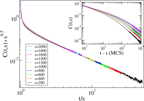
Figure 1: Critical aging scaling in Monte Carlo simulation data for the two-time density auto-correlation function in the Katz–Lebowitz–Spohn model on a $125,000\times 50$ rectangular lattice following a quench from a high-temperature disordered configuration. The inset shows the same data plotted as function of the time difference $t-s$, demonstrating broken time translation invariance (Figure reproduced with permission from: G.L. Daquila, 2011 Ph.D. dissertation, Virginia Tech).

Moreover, the associated upper critical dimensions of these models differ; for dimensional analysis with $[q_{\parallel}]=[{\vec{q}}_{\perp}]^{2}=\mu^{2}$ and $[c]=\mu^{0}$ gives for the driven Ising lattice gas $[S({\vec{x}},t)]=\mu^{-1+d/2}$ and consequently $[{\tilde{u}}]=\mu^{3-d}$, $[g]=\mu^{(5-d)/2}$. Therefore $d_{c}=5$, and the static non-linearity ${\tilde{u}}$ is irrelevant as compared with the drive $g$. While it may be omitted for the determination of the asymptotic universal scaling laws, at least in scaling functions one may not simply set ${\tilde{u}}=0$, since this dangerously irrelevant coupling is of course responsible for the occurrence of the phase transition. As in the non-critical driven lattice gas, the transverse sector is not affected by the drive non-linearity, and hence characterized by Gaussian model B critical exponents $\eta=0$, $\nu=1/2$, and $z=4$ in 23. In addition, Galilean invariance 29. holds and for $d\leq d_{c}=5$ implies the exact anisotropy exponent $\Delta=(8-d)/3$, and therefrom $\nu_{\parallel}=\nu\,(1+\Delta)=(11-d)/6$ and $z_{\parallel}=z/(1+\Delta)=12/(11-d)$ [75, 76, 64, 13]. Numerically, even on properly constructed anisotropic simulation domains, exceedingly long crossover times leading towards the asymptotic stationary scaling regime prohibit accurate determination of the critical exponents in driven Ising lattice cases [77]. Yet satisfactory dynamic aging scaling collapse can be achieved for the two-time density autocorrelation function with $\lambda_{C}=d-2+\eta+\Delta=2\,(d+1)/3$, as demonstrated in the Monte Carlo simulation data in Fig. 1 [78, 13].

5.2 Driven Interfaces: Kardar–Parisi–Zhang Model and Variants

Generic scale invariance emerges remarkably frequently in out-of-equilibrium systems. Aside from driven lattice gases, prominent examples include moving interfaces, pulled or pushed through materials by external driving, as well as surface growth under non-equilibrium conditions [79, 80, 81, 82]. For isotropic materials or substrates, and in the absence of long-range correlations in the thermal noise or random particle deposition processes, the scaling behavior of these systems is generically described by the Kardar–Parisi–Zhang model [83], captured by the non-linear Langevin equation

$$\frac{\partial S({\vec{x}},t)}{\partial t}=D\,{\vec{\nabla}}^{2}S({\vec{x}},t)+\frac{D\,g}{2}\left[{\vec{\nabla}}S({\vec{x}},t)\right]^{2}+\zeta({\vec{x}},t)\ ,$$ (32)

$$\big{\langle}\zeta({\vec{x}},t)\big{\rangle}=0\ ,\quad\left\langle\zeta({\vec{x}},t)\,\zeta({\vec{x}\,}^{\prime},t^{\prime})\right\rangle=2D\,\delta({\vec{x}}-{\vec{x}\,}^{\prime})\,\delta(t-t^{\prime})\ .$$ (33)

The scalar field $S({\vec{x}},t)$ represents the interface or surface height fluctuations relative to its mean position that moves or grows linear with time $t$. The $d$-dimensional substrate is parametrized by the coordinates ${\vec{x}}$, and a unique height profile function is surmised, i.e., any overhangs are neglected (or adequately coarse-grained). The non-linear term $\sim g$ describes curvature-driven propagation or growth. The height fluctuations are then scale-invariant at sufficiently large length scales up to $|{\vec{x}}|\leq L(t)\sim(D\,t)^{1/z}$ with dynamic exponent $z$. The dynamical height correlation function should thus obey the critical ($\tau=0$) scaling law 11., which in this context is usually written in terms of a roughness exponent $\chi$ [84]:

$$C({\vec{x}},t)=|{\vec{x}}|^{2\chi}\,{\hat{C}}(D\,t/|{\vec{x}}|^{z})\ ,\quad\chi=\frac{1}{2}\left(2-d-\eta\right)\,.$$ (34)

The associated linear growth model ($g=0$) or Edwards–Wilkinson equation [85] is just a noisy diffusion equation or Gaussian model A at criticality. Its effectively equilibrium kinetics tends towards the Gaussian stationary probability distribution

$${\cal P}_{s}[S]\sim\exp\left(-\frac{1}{2}\int\left[{\vec{\nabla}}S({\vec{x}})\right]^{2}d^{d}x\right)\,,$$ (35)

whence the corresponding scaling exponents are $\eta=0$ and $z=2$. The roughness exponent is therefore $\chi=1/2$ in one dimension, while the interface becomes flat ($\chi=0$) for $d\geq 2$. Indeed, $d_{c}=2$ represents the critical dimension for this problem, as can be inferred from direct scaling analysis: $[S({\vec{x}},t)]=\mu^{(d-2)/2}$, and $[g]=\mu^{1-d/2}$. Moreover, the substitution ${\vec{u}}({\vec{x}},t)=-{\vec{\nabla}}S({\vec{x}},t)$ transforms the Kardar–Parisi–Zhang equation to the $d$-dimensional noisy Burgers equation for a vorticity-free velocity field, ${\vec{\nabla}}\times{\vec{u}}({\vec{x}},t)=0$. The fluid dynamics invariance with respect to Galilean transformations, c.f. 29., maps onto (infinitesimal) tilt symmetry for the interface problem [86]: $S({\vec{x}},t)\to S^{\prime}({\vec{x}\,}^{\prime},t^{\prime})=S({\vec{x}}-D\,g\,{\vec{v}}\,t,t)-{\vec{v}}\cdot{\vec{x}}$. Since the height field scales with the roughness exponent $\chi$, demanding this invariance to hold under scale transformations enforces the scaling relation $\chi+z=2$.

Specifically in one dimension, the stationary distribution 35. pertains even to the non-linear Langevin equation 32., with the Hamiltonian just representing the Burgers fluid’s kinetic energy [86]. The ensuing exact exponent values $\eta=0$ and $\chi=1/2$ imply $z=3/2$, which of course coincides with the dynamical exponent $z_{\parallel}$ for the driven lattice gas. An explicit dynamic renormalization group analysis confirms these results [87, 88, 13]. It also allows an investigation of the non-equilibrium relaxation kinetics starting from an initially flat interface; the universal aging properties are again fully set by the stationary scaling exponents [89, 72, 90]. There are convincing experimental realizations for the Kardar–Parisi–Zhang scaling in $1+1$ dimensions that range from non-equilibrium surface growth, e.g., in electrodeposition [91], to flame front propagation in slow paper combustion [92], and turbulent dynamics in the electroconvection of nematic liquid crystals [93, 94]; data and scaling plots for the latter are depicted in Fig. 2.

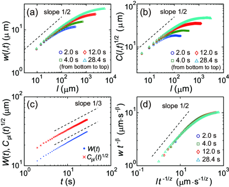
Figure 2: Experimental confirmation of Kardar–Parisi–Zhang dynamical scaling in electroconvective front propagation in turbulent nematic liquid crystals: (a) interface width $w(l,t)$ and (b) height difference correlation function $C(l,t)$ as function of length scale $l=|\vec{x}|$ for various times $t$ indicating initial growth with the roughness exponent $\chi=1/2$; (c) time evolution of the overall width $W(t)$ and the plateau level $C_{\rm pl}(t)$; and (d) Family–Vicsek scaling [84] collapse $w(l,t)=t^{\beta}{\hat{w}}(l\,t^{-1/z})$ with $\beta=\chi/z=1/3$. (Figures reproduced with permission from Ref. [93], DOI: 10.1103/PhysRevLett.104.230601; copyright 2010 by the American Physical Society).

In dimensions $d\geq d_{c}=2$, the Kardar–Parisi–Zhang equation displays even richer behavior, namely a non-equilibrium roughening transition that separates a smooth interface governed by the linear Edwards–Wilkinson equation from a rough phase, for which the non-linear coupling $g$ diverges in a perturbative renormalization group analysis [86, 87, 95, 96, 97, 71]. The scaling properties of this strong-coupling rough phase can however be successfully accessed through a non-perturbative numerical renormalization group approach [98, 99, 100]. Note that $d_{c}=2$ thus plays the role of a lower critical dimension for the existence of the roughening phase transition. Intriguingly, the Cole–Hopf transformation $S({\vec{x}},t)=k_{\rm B}T\,\ln Z({\vec{x}},t)/D\,g\,\varepsilon$ [95, 96, 97, 71] maps the stochastic differential equation 32. with additive white noise 33. to an imaginary-time Schrödinger equation for the canonical partition function $Z({\vec{x}},t)$ of a directed polymer, described by its trajectory ${\vec{x}}(t)$ along the $t$ direction, and with elastic line tension $\varepsilon$ at temperature $T$ that is subject to a Gaussian-distributed, spatially uncorrelated random pinning potential [101, 102, 103]. A simple scaling argument that demands that the elastic and pinning energies should both scale marginally at the roughening transition gives the critical exponent values $\chi_{c}=0$ and $z_{c}=2$ [104]. This can be confirmed in a computation to all orders in a dimensional $d=2+\epsilon$ expansion, along with the correlation length exponent $\nu_{c}=1/(d-2)$ [95, 97, 71, 13].

These considerations form the basis for more detailed investigations of the collective statistical mechanics and dynamics of interacting directed polymers in random media [105], with technologically relevant applications to the vortex and Bragg glass phases in type-II superconductors with point pinning centers [106]. Other broad extension include the non-equilibrium dynamics of extended elastic manifolds driven through random media [107, 108] that display continuous depinning transitions, whose theoretical analysis requires functional renormalization group tools [109], featuring scale-invariant avalanche kinetics [110].

It turns out that anisotropies in the non-linear growth and relaxation terms, which would naturally be expected to occur in real surfaces, constitute relevant perturbations for the Kardar–Parisi–Zhang equation in dimensions $d>2$, and lead to rich phenomena that include the possibility of first-order roughening transitions and multi-critical behavior [111]. The anisotropic Kardar–Parisi–Zhang equation also describes driven-dissipative Bose–Einstein condensation in two dimensions [112]. In many experiments on growing surfaces under non-equilibrium conditions, surface diffusion plays a crucial role to relax spatial inhomogeneities. Akin to model B for diffusive relaxational critical dynamics, so-called conserved Kardar–Parisi–Zhang model variants thus incorporate an additional Laplacian $-{\vec{\nabla}}^{2}$ in front of the systematic contributions to the Langevin equation 32.; since the noise correlations are not constrained by a fluctuation-dissipation relation, one may then either consider the Sun–Gao–Grant model with conserved ($a=2$) noise [113], or the Wolf–Villain model with non-conserved ($a=0$) shot noise [114]. In either case, the dynamic scaling exponent becomes $z=4-\eta$, and is related to the roughness exponent via the scaling relation $\chi=(z-a-d)/2=(4-a-d-\eta)/2$ [115, 13].

6 REACTING PARTICLE SYSTEMS: SCALING AND PHASE TRANSITIONS

This final section describes scale-invariant correlation-dominated relaxation kinetics in reacting particle systems [116, 117, 118], and discusses active-to-absorbing state transitions in reaction-diffusion and simple epidemic or population dynamics models [119, 120, 121, 13].

6.1 Scale Invariance in Diffusion-Limited Reactions

In chemical reactions, individual particles of species $A,B,\ldots$ are annihilated, created, or transformed either spontaneously or upon encounter with certain rates. Since particle numbers are changed by integer numbers $\{n_{\alpha}\}$ in these stochastic processes, the corresponding loss and gain terms in the associated master equations can be expressed through the action of bosonic creation and annihilation operators on a Fock space state vector $|\{n_{\alpha}\}\rangle$ that contains a list of all species’ particle occupations [122, 123, 124]. One may then utilize a coherent-state basis for the resulting non-Hermitean many-body problem to construct an equivalent Doi–Peliti path-integral representation [125, 126, 127, 128, 13]. If the occupation numbers are restricted to just $n_{\alpha}=0$ or $1$, the stochastic reactions can in contrast be represented through spin-$1/2$ operators. This mapping is especially fruitful in one dimension, where mathematical tools such as the Bethe ansatz developed for quantum spin chains can be applied to the ensuing non-Hermitean spin Hamiltonians [129, 130, 131, 67].

For at most binary reactions, the path integral action can be cast in the form 18. albeit with complex fields $\psi^{\alpha}({\vec{x}},t)$; $F^{\alpha}[\psi]$ then represents the reaction functional as familiar from the mass action expression or chemical rate equation in well-mixed systems. One may therefore write down an effective coarse-grained Langevin description, with usually multiplicative internal reaction noise encoded in the functional $L^{\alpha}[\psi]$. Let us consider the simplest scenario, namely diffusing particles of species $A$ subject to the annihilation processes $k\,A\to l\,A$ where $0\leq l<k\leq 2$. With continuum diffusion and reaction rates $D$ and $\lambda$, the ensuing stochastic partial differential equation becomes [132, 133, 126, 13]

$$\frac{\partial\psi({\vec{x}},t)}{\partial t}=D\,{\vec{\nabla}}^{2}\,\psi({\vec{x}},t)-(k-l)\,\lambda\,\psi({\vec{x}},t)^{k}+\zeta({\vec{x}},t)\ ,$$ (36)

with $\langle\zeta({\vec{x}},t)\rangle=0$ and the formal noise correlator

$$\left\langle\zeta({\vec{x}},t)\,\zeta({\vec{x}\,}^{\prime},t^{\prime})\right\rangle=-2\left[k(k-1)-l(l-1)\right]\lambda\,\psi({\vec{x}},t)^{k}\,\delta({\vec{x}}-{\vec{x}\,}^{\prime})\,\delta(t-t^{\prime})\ .$$ (37)

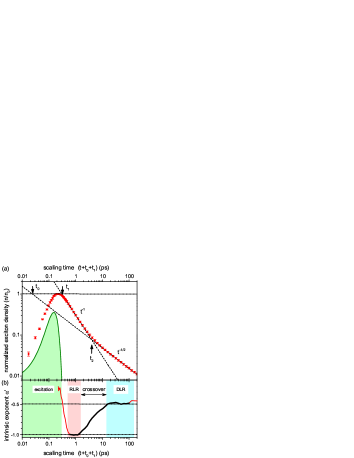
Figure 3: Experimental exciton recombination data in single-walled carbon nanotubes that clearly demonstrate the crossover from reaction- to diffusion-limited power law decay: (a) normalized exciton density as function of time; (b) the intrinsic effective decay exponent displays plateaus at the reaction-limited value $-1$ and renormalized diffusion-limited $-1/2$ (Figures reproduced with permission from Ref. [137], DOI: 10.1103/PhysRevLett.111.197401; copyright 2013 by the American Physical Society).

For $k=1$, i.e., spontaneous death $A\to\emptyset$ at rate $\lambda$, the stochastic noise vanishes, and the mean particle density of course decays exponentially, $a(t)=\langle\psi({\vec{x}},t)\rangle=a(0)\,e^{-\lambda\,t}$. In contrast, the negative sign in 37. for $k=2$ indicates emerging spatial anti-correlations, as the pair annihilation reactions quickly remove near-by particles. Neglecting temporal fluctuations and spatial correlations, i.e., omitting the noise and diffusive spreading in 36., the ensuing mean-field rate equation for the particle density is for $k\geq 2$ solved by $a(t)=\left[a(0)^{1-k}+(k-l)(k-1)\,\lambda\,t\right]^{-1/(k-1)}$, which asymptotically yields a power law decay that is independent of the initial value $a(0)$. Since the field $[\psi({\vec{x}},t)]=\mu^{d}$ should scale like a density, one obtains the scaling dimension $[\lambda]=\mu^{2-(k-1)d}$ for the $k$-th order annihilation rate. Consequently the critical dimension for stochastic annihilation is $d_{c}(k)=2/(k-1)$; for $k\geq 4$ therefore, fluctuations do not markedly modify the mean-field reaction-limited decay law in any physical dimension $d$. For pair ($k=2$) annihilation $A+A\to\emptyset$ or coagulation $A+A\to A$, the reactions generate spatial depletion zones of typical length $L(t)$ that need to be traversed diffusively by other particles before further annihilations can ensue. In this diffusion-limited regime, therefore $L(t)\sim(Dt)^{1/2}$, whence $a(t)\sim L(t)^{-d}\sim(D\,t)^{-d/2}$, which represents a slower decay than the reaction-limited $a(t)\sim(\lambda\,t)^{-1}$ in dimensions $d\leq 2$ [132, 133, 126, 118]. Precisely at the critical dimension $d_{c}(2)=2$, and $d_{c}(3)=1$ for triplet annihilation, one obtains logarithmic corrections: $a(t)\sim\left[(D\,t)^{-1}\,\ln(D\,t)\right]^{1/(k-1)}$. Experimentally, the anomalous diffusion-limited power law decay in one dimension has been verified in the exciton recombination kinetics in molecular wires [134], TMMC polymer chains [135], and carbon nanotubes [136]; the convincing data from Ref. [137] shown in Fig. 3 provide clear evidence for the crossover from the reaction- to diffusion-limited regimes.

Additional and quite different physical mechanisms govern the emerging spatial correlations in two-species pair annihilation $A+B\to\emptyset$, where crucially the particle number difference of the two species remains conserved under the time evolution [138]. With equal diffusivities for both species, the associated stochastic differential equations read [139, 13]

$$\frac{\partial\psi({\vec{x}},t)}{\partial t}=D{\vec{\nabla}}^{2}\psi({\vec{x}},t)-\lambda\,\psi({\vec{x}},t)\,\varphi({\vec{x}},t)+\zeta({\vec{x}},t)\ ,$$

$$\frac{\partial\varphi({\vec{x}},t)}{\partial t}=D{\vec{\nabla}}^{2}\varphi({\vec{x}},t)-\lambda\,\psi({\vec{x}},t)\,\varphi({\vec{x}},t)+\eta({\vec{x}},t)\ ,$$ (38)

with $\langle\zeta({\vec{x}},t)\rangle=0=\langle\eta({\vec{x}},t)\rangle$ and the noise (cross-)correlations

$$\langle\zeta({\vec{x}},t)\,\zeta({\vec{x}\,}^{\prime},t^{\prime})\rangle=0=\langle\eta({\vec{x}},t)\,\eta({\vec{x}\,}^{\prime},t^{\prime})\rangle\ ,$$

$$\langle\zeta({\vec{x}},t)\,\eta({\vec{x}\,}^{\prime},t^{\prime})\rangle=-\lambda\,\psi({\vec{x}},t)\,\varphi({\vec{x}},t)\,\delta({\vec{x}}-{\vec{x}\,}^{\prime})\,\delta(t-t^{\prime})\ .$$ (39)

For unequal initial densities $a(0)-b(0)=a(\infty)>0$, only the majority species $A$ will survive as $t\to\infty$, and in dimensions $d>2$, the approach to the stationary values is exponential: $a(t)-a(\infty)\sim b(t)\sim e^{-\lambda\,a(\infty)\,t}$. In low dimensions $d<2$, depletion zone anti-correlations induce a slower, stretched-exponential decay, $\ln\left[a(t)-a(\infty)\right]\sim\ln b(t)\sim-(Dt)^{d/2}$, whereas at $d_{c}=2$ one obtains $\ln\left[a(t)-a(\infty)\right]\sim\ln b(t)\sim-Dt/\ln(Dt)$. In stark contrast, for equal initial densities $a(0)=b(0)$, the mean-field rate equations predict $a(t)\sim b(t)\sim(\lambda\,t)^{-1}$ as for single-species pair annihilation. This becomes modified by spatial particle species segregation in dimensions $d\leq d_{s}=4$; exploiting that $c({\vec{x}},t)=\psi({\vec{x}},t)-\varphi({\vec{x}},t)$ becomes a purely diffusive mode, straightforward analysis shows that the local density excess decays slowly, $|c(x,t)|=2\sqrt{a(0)/\pi}\,(8\pi\,D\,t)^{-d/4}$, whence also $a(t)\sim b(t)\sim(D\,t)^{-d/4}$. The annihilation reactions become confined to narrow reaction zones that separate segregated and inert $A$ and $B$ domains. The reaction zone width scales as $w(t)\sim(D\,t)^{\Lambda}$, where $\Lambda=1/3$ in the mean-field approximation, while $\Lambda=(d+2)/4\,(d+1)$ for $d\leq d_{c}=2$. The three-dimensional non-classical decay $\sim t^{-3/4}$ has been observed experimentally [140].

Note that the highly correlated alternating initial arrangement $\ldots ABABABABAB\ldots$ is preserved by the reactions $A+B\to\emptyset$ in one dimension; hence the distinction between $A$ and $B$ particles becomes meaningless, and their densities indeed satisfy the single-species $t^{-1/2}$ pair annihilation power law. One may in fact fully analyze the $q$-species pair annihilations $A_{i}+A_{j}\to\emptyset$, $1\leq i<j\leq q$, with equal initial densities $a_{i}(0)$ as well as uniform diffusion and reaction rates [141, 142, 143]. Indeed, for more than two species ($q>2$), there exists no conservation law in the stochastic kinetics, and species segregation results for $d<d_{s}(q)=4/(q-1)$. For $d\geq 2$, one therefore obtains the single-species pair annihilation decay laws. On one dimension, each species’ density obeys $a_{i}(t)\sim t^{-\alpha(q)}+C\,t^{-1/2}$, i.e., a leading slow power law decay with $\alpha(q)=(q-1)/2q$ induced by segregation effects, accompanied with a subleading term caused by depletion zones. For the reaction front width, one finds the scaling behavior $w(t)\sim t^{\Lambda(q)}$ with $\Lambda(q)=(2q-1)/4q$.

6.2 Active-to-Absorbing State Phase Transitions

If in addition to particle decay $A\to\emptyset$ and annihilations, e.g., $A+A\to A$, one allows for competing offspring production through branching processes such as $A\to A+A$, the overall particle density may at long times either reach a finite mean value, representing an active state, or vanish. In situations where the presence of particles is required for any generation of further offspring, i.e., in the absence of spontaneous particle production $\emptyset\to A$, the latter inactive phase is also absorbing: Once reached, there are no stochastic processes available that would allow the system to escape this empty state [119, 120, 121]. Although we have just formulated the active-to-absorbing transition scenario in terms of chemical reactions, the particle-like excitations could also be domain walls that coalesce or annihilate, or other effective coarse-grained degrees of freedom whose kinetics is captured by these stochastic interactions. More generally, one may consider spreading activity fronts or an infectious epidemic which on a lattice would be represented by discrete entities $A$.

Indeed, heuristic considerations permit a straightforward phenomenological continuum description of the so-called simple epidemic process or a spreading epidemic with recovery [144]: Assuming diffusive spreading with diffusion constant $D$, and strictly local infections of a homogeneous susceptible medium, we write down the Langevin equation [145, 13]

$$\frac{\partial S({\vec{x}},t)}{\partial t}=D\,{\vec{\nabla}}^{2}S({\vec{x}},t)-R[S({\vec{x}},t)]\,S({\vec{x}},t)+\zeta({\vec{x}},t)\ ,$$ (40)

where $R[S]$ denotes an appropriate reaction functional with finite limit as the active or infected density $S\to 0$. In addition, the and multiplicative stochastic noise with vanishing mean $\langle\zeta({\vec{x}},t)\rangle=0$ and correlator

$$\left\langle\zeta({\vec{x}},t)\,\zeta({\vec{x}\,}^{\prime},t^{\prime})\right\rangle=2L[S({\vec{x}},t)]\,\delta({\vec{x}}-{\vec{x}\,}^{\prime})\,\delta(t-t^{\prime})$$ (41)

that represents all other fast degrees of freedom and internal reaction noise must also satisfy the absorbing-state condition, whence $L[S]\to 0$ as $S\to 0$. In the vicinity of the extinction threshold, we may approximate both reaction and noise functionals in the spirit of a Landau expansion: $R[S]=D\,r+u\,S\,+\ldots$ and $L[S]=v\,S+\ldots$. After straightforward rescaling, we may set $v=u$; dimensional analysis with $[S({\vec{x}},t)]=\mu^{d/2}$ and $[D]=\mu^{0}$ then yields $[r]=\mu^{2}$ and $[u]=\mu^{2-d/2}$. Thus $d_{c}=4$ is the upper critical dimension for the absorbing-state phase transition, and omitting higher-order terms as well as powers of gradients of the activity field become a-posteriori justified, since all such additional contributions turn out to be irrelevant in the renormalization group sense. Neglecting the multiplicative noise, 40. reduces to the deterministic Fisher–Kolmogorov reaction-diffusion equation [146, 144]. The phase transition to the absorbing state occurs at $r=0$; in the active state for $r<0$ one has $\phi(\infty)=D\,|r|/u$ as $t\to\infty$ or $\beta=1$; diffusive propagation implies $z=2$, and the mean-field critical correlation exponents are $\eta=0$ and $\nu=1/2$. Precisely at the extinction threshold, the mean density decays algebraically: $\phi(t)=\langle S({\vec{x}},t)\rangle\sim t^{-\alpha}$ with $\alpha=\beta/z\,\nu$.

The Janssen–De Dominicis response functional 18. for the stochastic differentical equation 40. with multiplicative noise 41. and just the leading and relevant terms retained in the functional expansions is known as Reggeon field theory [147]; it in turn represents the effective action for the universal scaling properties of directed percolation [148]: Here, the time coordinate maps onto a singled-out spatial direction, and the decay, annihilation, and reproduction processes respectively correspond to terminal, coalescing, or splitting branches in the ensuing percolation clusters [149]. Its characteristic symmetry feature is rapidity invariance, which entails time inversion and exchange of the dynamical fields: $S({\vec{x}},t)\leftrightarrow-{\widetilde{S}}({\vec{x}},-t)$. These considerations establish the Janssen–Grassberger conjecture, which states that the asymptotic critical features for continuous non-equilibrium phase transitions from active to inactive, absorbing states that are described by a scalar order parameter field and governed by Markovian stochastic dynamics that is decoupled from any other slow variables and not subject to the influence of quenched disorder, are generically captured by the universality class of directed percolation [150, 151]. The associated critical and aging scaling exponents are numerically known to high accuracy in all dimensions $d<d_{c}=4$ [121], and can be systematically computed in a $d=4-\epsilon$ expansion by means of the perturbative dynamical renormalization group [145, 13]. Experimentally, directed percolation scaling has been observed in intermittent ferrofluidic spikes [152], and unambiguously at the transition between different turbulent states of electro-hydrodynamic convection in thin nematic liquid crystals [153, 154]. Figure 4 shows the active density decay near criticality and data collapse obtained with directed percolation scaling exponents.

While coupling to other slow modes or quenched randomness in the percolation threshold may invalidate directed percolation scaling [121], this universality class still pertains for an extension of active-to-absorbing state transitions to multiple particle species [155, 156], except for special multi-critical points in parameter space [157, 158]. For example, in spatially extended stochastic Lotka–Volterra predator-prey models [146, 144], local restrictions of the prey carrying capacity induces a predator extinction threshold. This continuous transition displays directed-percolation critical exponents, and its effective Doi–Peliti action can be mapped to Reggeon field theory [159, 160]. Numerical simulations confirm that population extinctions are generically described by the directed percolation scaling laws, including the associated critical aging exponents [159, 161]. Another remarkable analogy addresses the onset of shear turbulence in pipe flow, which displays very similar spatio-temporal phenomena as predator-prey kinetics, including spreading activity fronts; its threshold properties have hence been argued to belong to the directed-percolation universality class as well [162].

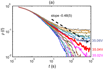
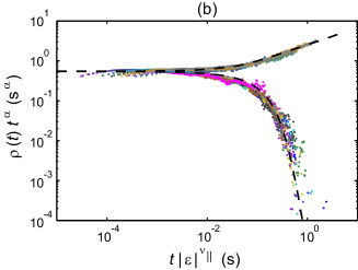
Figure 4: Evidence for directed percolation critical behavior in effectively two-dimensional turbulent liquid crystals: (a) active density decay in the vicinity of the critical voltage; (b) scaling collapse with critical exponents $\alpha\approx 0.48$ and $\nu_{\parallel}\approx 1.29$; the thick dashed lines indicate the scaling functions in the active (upper curve) and absorbing (lower curve) phases obtained from contact process Monte Carlo simulations (Figures reproduced with permission from Ref. [154], DOI: 10.1103/PhysRevE.80.051116; copyright 2009 by The American Physical Society).

In general epidemic processes [144], infected sites or individuals never return to a susceptible state, but remain infectious to their neighbors. This induces persistent temporal memory into the non-linearity in 40. of the form $D\,u\,S({\vec{x}},t)\int_{-\infty}^{t}S({\vec{x}},t^{\prime})\,dt^{\prime}$ [163, 164, 165]. This enhances the influence of correlations and shifts the upper critical dimension to $d_{c}=6$; interestingly, the ensuing quasi-static scaling properties near the infection threshold are identical to those for static isotropic percolation clusters [166]. Active-to-absorbing state transitions also occur in branching and annihilating random walks wherein diffusing particles are subject to the competing reactions $A+A\to\emptyset$ and $A\to(m+1)\,A$ with integer $m$ [167, 168]. Here, the situations of odd or even $m$ are crucially different: For odd $m=1,3,\ldots$, fluctuations that combine both these processes generate the spontaneous decay $A\to\emptyset$, and the phase transition is governed by directed-percolation scaling exponents. However, that is not possible for branching reactions with even $m=2,4,\ldots$, as in this case the particle number parity is a locally conserved quantity. In fact, the entire absorbing state of this parity-conserving universality class is characterized by the pure binary-annihilation decay laws, and hence by scale-invariant dynamical correlations. It actually constitutes a special case for a generalized voter model universality class that obeys a $Z_{2}$ inversion symmetry [169]. Replacing first-order branching with the binary reaction $A+A\to(m+2)\,A$ yields the pair contact process with diffusion. If arbitrarily many particles are allowed per lattice site, it displays a strongly discontinuous non-equilibrium phase transition [170]; in contrast, if site occupation restrictions are implemented, its absorbing state transition becomes continuous, but owing to exceedingly long crossovers, its precise asymptotic scaling properties are still controversial [171]. Despite extensive efforts, e.g. [172], a full classification of active-to-absorbing phase transitions that incorporate triplet or higher-order reactions has remained elusive to date.

7 CONCLUSION AND OUTLOOK

Below, I list the main conclusions of this brief (and by necessity incomplete) introductory overview on continuous phase transitions and the emergence of dynamical scaling in non-equilibrium systems, and provide my personal outlook to crucial future research avenues.

[SUMMARY POINTS]

1. In thermal equilibrium, universality classes for critical dynamics are defined through the symmetries of the order parameter, conservation laws, and possible couplings of the order parameter to other slow conserved modes.

2. Dynamical scaling concepts have been successfully extended to quantum phase transitions and open systems far from equilibrium.

3. Aging scaling emerges in the non-equilibrium relaxation kinetics of systems with either exceedingly long relaxation times or slow algebraic decay.

4. Generic scale invariance is a quite prevalent feature of non-equilibrium stationary states in driven systems.

5. Driven-diffusive systems are characterized by anisotropic scaling laws.

6. The Kardar–Parisi–Zhang model and variants describe universal scaling features and a non-equilibrium roughening transition of driven interfaces or growing surfaces.

7. In diffusion-limited reacting particle systems at low dimensions, strong temporal fluctuations and spatial correlations invalidate standard mean-field rate equation descriptions that utilize mass-action type factorizations.

8. Active-to-absorbing state transitions are generically captured by the universal scaling properties of critical directed percolation.

[FUTURE ISSUES]

1. Reproducible and quantitative experimental verification based on top-quality data of the theoretically and numerically established prominent dynamical universality classes out of equilibrium currently only exists for a few important cases (e.g., diffusion-limited annihilation, Kardar–Parisi–Zhang scaling, directed percolation).

2. A full classification of all possible non-equilibrium universality classes remains elusive to date, owing to the increasing complexity as additional relevant degress of freedom or reacting particle or ecological species are taken into consideration.

3. The emergence of improved quantitative data in biological systems ranging from biochemical reactions via collective behavior of micro-organisms to macroscopic pattern formation and population extinctions in eco-systems promises to become an ever more fertile ground for the application of scaling tools from statistical physics.

DISCLOSURE STATEMENT

The author is not aware of any affiliations, memberships, funding, or financial holdings that might be perceived as affecting the objectivity of this review.

References

- [1] Fisher ME. 1967. Rep. Prog. Phys. 30:615–730
- [2] Stanley HE. 1971. Introduction to Phase Transitions and Critical Phenomena. Oxford: Clarendon Press
- [3] Ma S. 1976. Modern Theory of Critical Phenomena. Reading: Benjamin-Cummings
- [4] Yeomans JM. 1991. Statistical Mechanics of Phase Transitions. Oxford: Clarendon Press
- [5] Goldenfeld N. 1992. Lectures on Phase Transitions and the Renormalization Group. Reading: Addison-Wesley
- [6] Binney JJ, Dowrick NJ, Fisher AJ, Newman MEJ. 1993. The Theory of Critical Phenomena. Oxford: Oxford Univ. Press. 2nd ed.
- [7] Chaikin PM, Lubensky TC. 1995. Principles of Condensed Matter Physics. Cambridge: Cambridge Univ. Press
- [8] Cardy J. 1996. Scaling and Renormalization in Statistical Physics. Cambridge: Cambridge Univ. Press
- [9] Amit DJ. 1984. Field Theory, the Renormalization Group, and Critical Phenomena. Singapore: World Scientific
- [10] Itzykson C, Drouffe JM. 1989. Statistical Field Theory, Vols. I, II. Cambridge: Cambridge Univ. Press
- [11] Zinn-Justin J. 1993. Quantum Field Theory and Critical Phenomena. Oxford: Clarendon Press
- [12] Vasil’ev AN. 2004. The Field Theoretic Renormalization Group in Critical Behavior Theory and Stochastic Dynamics. Boca Raton: Chapman & Hall / CRC Publ.
- [13] Täuber UC. 2014. Critical Dynamics – A Field Theory Approach to Equilibrium and Non-Equilibrium Scaling Behavior. Cambridge: Cambridge Univ. Press
- [14] Ferrell RA, Menyhàrd N, Schmidt H, Schwabl F, Szépfalusy P. 1967. Phys. Rev. Lett. 18:891–894
- [15] Ferrell RA, Menyhàrd N, Schmidt H, Schwabl F, Szépfalusy P. 1968. Ann. Phys. (NY) 47:565–613
- [16] Halperin BI, Hohenberg PC. 1969. Phys. Rev. 177:952–971
- [17] Hohenberg PC, Halperin BI. 1977. Rev. Mod. Phys. 49:435–479
- [18] Folk R, Moser G. 2006. J. Phys. A: Math. Gen. 39:R207–R313
- [19] Forster D. 1983. Hydrodynamic Fluctuations, Broken Symmetry, and Correlation Functions. Redwood City: Addison-Wesley. 3rd ed.
- [20] Lovesey SW. 1986. Condensed Matter Physics: Dynamic Correlations. Menlo Park: Benjamin-Cummings. 2nd. ed.
- [21] Kubo R, Toda M, Hashitsume N. 1991. Statistical Physics II – Nonequilibrium Statistical Mechanics. Berlin: Springer Verlag. 2nd ed.
- [22] Van Vliet CM. 2010. Equilibrium and Non-equilibrium Statistical Mechanics. New Jersey: World Scientific. 2nd ed.
- [23] Continentino MA. 1994. Phys. Rep. 239:179–213
- [24] Vojta M. 2003. Rep. Prog. Phys. 66:2069–2110
- [25] Sachdev S. 2011. Quantum Phase Transitions. Cambridge: Cambridge Univ. Press. 2nd ed.
- [26] Negele JW, Orland J. 1988. Quantum Many-Particle Systems. Redwood City: Addison-Wesley
- [27] Risken H. 1984. The Fokker–Planck Equation. Heidelberg: Springer Verlag
- [28] Schwabl F. 2006. Statistical Mechanics. Berlin: Springer Verlag. 2nd ed.
- [29] Deker U, Haake F. 1975. Phys. Rev. A 11:2043–2056
- [30] De Dominicis C. 1976. J. Phys. (France) Colloq. C1:C247–C253
- [31] Janssen HK. 1976. Z. Phys. B 23:377–380
- [32] Bausch R, Janssen HK, Wagner H. 1976. Z. Phys. B Cond. Matt. 24:113–127
- [33] Janssen HK. 1979. In: Dynamical Critical Phenomena and Related Topics, Lecture Notes in Physics 104:26–47. Ed. Enz CP. Heidelberg: Springer Verlag
- [34] Kamenev A. 2011. Field Theory of Non-Equilibrium Systems. Cambridge: Cambridge Univ. Press
- [35] Sieberer LM, Buchhold M, Diehl S. 2016. Rep. Prog. Phys. 79:096001-1–68
- [36] Folk R, Moser G. 2003. Phys. Rev. Lett. 91:030601-1–4
- [37] Folk R, Moser G. 2004. Phys. Rev. E 69:036101-1–18
- [38] Haake F, Lewenstein M, Wilkens M. 1984. Z. Phys. B Cond. Matt. 55:211–218
- [39] Grinstein G, Jayaprakash C, He Y. 1985. Phys. Rev. Lett. 55:2527–2530
- [40] Bassler KE, Schmittmann B. 1994. Phys. Rev. Lett. 73:3343–3346
- [41] Risler T, Prost J, Jülicher F. 2005. Phys. Rev. E 72:016130-1–18
- [42] Cross MC, Hohenberg PC. 1993. Rev. Mod. Phys. 65:851–1112
- [43] Cross M, Greenside H. 2009. Pattern Formation and Dynamics in Nonequilibrium Systems. Cambridge: Cambridge Univ. Press
- [44] Frey E. 2010. Physica A 389:4265–4298
- [45] Sieberer LM, Huber SD, Altman E, Diehl S. 2013. Phys. Rev. Lett. 110:195301-1–5
- [46] Sieberer LM, Huber SD, Altman E, Diehl S. 2014. Phys. Rev. B 89:134310-1–34
- [47] Täuber UC, Diehl S. 2014. Phys. Rev. X 4:021010-1–21
- [48] Täuber UC, Rácz Z. 1997. Phys. Rev. E 55:4120–4136
- [49] Täuber UC, Santos JE, Rácz Z. 1999. Eur. Phys. J. B 7:309–330
- [50] Täuber UC, Akkineni VK, Santos JE. 2002. Phys. Rev. Lett. 88:045702-1–4
- [51] Schmittmann B, Zia RKP. 1991. Phys. Rev. Lett. 66:357–360
- [52] Schmittmann B. 1993. Europhys. Lett. 24:109–114
- [53] Schwabl F, Täuber UC. 1996. Phil. Trans. R. Soc. Lond. A 354:2847–2873
- [54] Santos JE, Täuber UC. 2002. Eur. Phys. J. B 28:423–440
- [55] Akkineni VK, Täuber UC. 2004. Phys. Rev. E 69:036113-1–25
- [56] Henkel M, Pleimling M. 2010. Non-Equilibrium Phase Transitions. Vol 2: Ageing and Dynamical Scaling Far From Equilibrium. Dordrecht: Springer Verlag
- [57] Bray AJ. 1994. Adv. Phys. 43:357–459
- [58] Janssen HK, Schaub B, Schmittmann B. 1989. Z. Phys. B Cond. Matt. 73:539–549
- [59] Janssen HK. 1992. In: From Phase Transitions to Chaos:68–91. Eds. Györgyi G, Kondor I, Sasvári L, Tél T. Singapore: World Scientific
- [60] Calabrese P, Gambassi A. 2005. J. Phys. A: Math. Gen. 38:R133–R193
- [61] Oerding K, Janssen HK. 1993. J. Phys. A: Math. Gen. 26:3369–3381
- [62] Oerding K, Janssen HK. 1993. J. Phys. A: Math. Gen. 26:5295–5303
- [63] Zheng B. 1998. Int. J. of Mod. Phys. B 12:1419–1484.
- [64] Schmittmann B, Zia RKP. 1995. Phase Transitions and Critical Phenomena. Vol. 17. Eds. Domb C, Lebowitz JL. London: Academic Press
- [65] Marro J, Dickman R. 1999. Nonequilibrium Phase Transitions in Lattice Models. Cambridge: Cambridge Univ. Press
- [66] Derrida B. 1998. Phys. Rep. 301:65–83
- [67] Stinchcombe R. 2001. Adv. Phys. 50:431–496
- [68] Chou T, Mallick K, Zia RKP. 2011. Rep. Prog. Phys. 74:116601-1–41
- [69] Janssen HK, Schmittmann B. 1986. Z. Phys. B Cond. Matt. 63:517–520
- [70] Forster D, Nelson DR, Stephen MJ. 1977. Phys. Rev. A 16:732–749
- [71] Janssen HK, Täuber UC, Frey E. 1999. Eur. Phys. J. B 9:491–511
- [72] Daquila GL, Täuber UC. 2011. Phys. Rev. E 83:051107-1–11
- [73] Katz S, Lebowitz JL, Spohn H. 1983. Phys. Rev. B 28:1655–1658
- [74] Katz S, Lebowitz JL, Spohn H. 1984. J. Stat. Phys. 34:497–537
- [75] Janssen HK, Schmittmann B. 1986. Z. Phys. B Cond. Matt. 64:503–514
- [76] Leung K, Cardy JL. 1986. J. Stat. Phys. 44:567–588
- [77] Caracciolo S, Gambassi A, Gubinelli M, Pelissetto A. 2004. J. Stat. Phys. 115:281–322
- [78] Daquila GL, Täuber UC. 2012. Phys. Rev. Lett. 108:110602-1–5
- [79] Krug J, Spohn H. 1992. In: Solids far from equilibrium:479–582. Ed. Godrèche C. Cambridge: Cambridge Univ. Press
- [80] Barabási AL, Stanley HE. 1995. Fractal Concepts in Surface Growth. Cambridge: Cambridge Univ. Press
- [81] Halpin-Healy T, Zhang YC. 1995. Phys. Rep. 254:215–414
- [82] Krug J. 1997. Adv. Phys. (NY) 46:139–282
- [83] Kardar M, Parisi G, Zhang YC. 1986. Phys. Rev. Lett. 56:889–892
- [84] Family F, Vicsek T. 1985. J. Phys. A: Math. Gen. 18:L75–-L81
- [85] Edwards SF, Wilkinson DR. 1982. Proc. R. Soc. London A 381:17–31
- [86] Medina E, Hwa T, Kardar M, Zhang YC. 1989. Phys. Rev. A 39:3053–3075
- [87] Frey E, Täuber UC. 1994. Phys. Rev. E 50:1024–1045
- [88] Frey E, Täuber UC, Hwa T. 1996. Phys. Rev. E 53:4424–4438
- [89] Krech M. 1997. Phys. Rev. E 55:668–679
- [90] Henkel M, Noh JD, Pleimling M. 2012. Phys. Rev. E 85:030102(R)-1–5
- [91] Schilardi PL, Azzaroni O, Salvarezza RC, Arvia AJ. 1999. Phys. Rev. B 59:4638–4641
- [92] Myllys M, Maunuksela J, Alava M, Ala-Nissila T, Merikoski J, Timonen J. 2001. Phys. Rev. E 64:036101-1–12
- [93] Takeuchi KA, Sano M. 2010. Phys. Rev. Lett. 104:230601-1–4
- [94] Takeuchi KA, Sano M. 2012. J. Stat. Phys. 147:853–890
- [95] Lässig M. 1995. Nucl. Phys. B 448:559–574
- [96] Lässig M. 1998. J. Phys. Cond. Matt. 10:9905–9950
- [97] Wiese KJ. 1998. J. Stat. Phys. 93:143–154
- [98] Canet L, Chaté H, Delamotte B, Wschebor N. 2010. Phys. Rev. Lett. 104:150601-1–4
- [99] Canet L, Chaté H, Delamotte B, Wschebor N. 2011. Phys. Rev. E 84:061128-1–18
- [100] Kloss T, Canet L, Wschebor N. 2012. Phys. Rev. E 86:051124-1–19
- [101] Kardar M, Zhang YC. 1987. Phys. Rev. Lett. 58:2087–2090
- [102] Fisher DS, Huse DA. 1991. Phys. Rev. B 43:10728–10742
- [103] Hwa T, Fisher DS. 1994. Phys. Rev. B 49:3136–3154
- [104] Doty CA, Kosterlitz JM. 1992. Phys. Rev. Lett. 69:1979–1981
- [105] Kardar M. 1998. Phys. Rep. 301:85–112
- [106] Nattermann T, Scheidl S. 2000. Adv. Phys. 49:607–704
- [107] Balents L, Marchetti MC, Radzihovsky L. 1998. Phys. Rev. B 57:7705–7739
- [108] Fisher DS. 1998. Phys. Rep. 301:113–150
- [109] Le Doussal P, Wiese KJ, Chauve P. 2004. Phys. Rev. E 69:026112-1–42
- [110] Le Doussal P, Wiese KJ. 2013 Phys. Rev. E 88:022106-1–68
- [111] Täuber UC, Frey E. 2002. Europhys. Lett. 59:655–661
- [112] Altman E, Sieberer LM, Chen L, Diehl S, Toner J. 2015. Phys. Rev. X 5:011017-1–11
- [113] Sun T, Guo H, Grant M. 1989. Phys. Rev. A 40:6763–6766
- [114] Wolf DE, Villain J. 1990. Europhys. Lett. 13: 389–394
- [115] Janssen HK. 1997. Phys. Rev. Lett. 78:1082–1085
- [116] Kuzovkov V, Kotomin E. 1988. Rep. Prog. Phys. 51:1479–1523
- [117] Ovchinnikov AA, Timashev SF, Belyy AA. 1989. Kinetics of Diffusion-Controlled Chemical Processes. New York: Nova Science
- [118] Krapivsky PK, Redner S, Ben-Naim E. 2010. A kinetic view of statistical physics. Cambridge: Cambridge Univ. Press
- [119] Hinrichsen H. 2000. Adv. Phys. 49:815–958
- [120] Ódor G. 2004. Rev. Mod. Phys. 76:663–724
- [121] Henkel M, Hinrichsen H, Lübeck S. 2008. Non-Equilibrium Phase Transitions. Vol 1: Absorbing Phase Transitions. Dordrecht: Springer Verlag
- [122] Doi M. 1976. J. Phys. A: Math. Gen. 9:1465–1477; 9:1479–1495
- [123] Grassberger P, Scheunert M. 1980. Fortschr. Phys. 28:547–578
- [124] Mattis DC, Glasser ML. 1998. Rev. Mod. Phys. 70:979–1002
- [125] Peliti L. 1985. J. Phys. (Paris) 46:1469–1482
- [126] Täuber UC, Howard M, Vollmayr-Lee BP. 2005. J. Phys. A: Math. Gen. 38:R79–R131
- [127] Andreanov A, Biroli G, Bouchaud JP, Lefèvre A. 2006. Phys. Rev. E 74:030101-1–4
- [128] Cardy J. 2008. In: Non-Equilibrium Statistical Mechanics and Turbulence, London Math. Soc. Lecture Note Ser. 355: 108–161. Cambridge: Cambridge Univ. Press.
- [129] Alcaraz FC, Droz M, Henkel M, Rittenberg V. 1994. Ann. Phys. (NY) 230:250–302
- [130] Henkel M, Orlandini E, Santos J. 1997. Ann. Phys. (NY) 259:163–231
- [131] Schütz GM. 2001. Phase Transitions and Critical Phenomena. Vol. 19. Eds. Domb C, Lebowitz JL. London: Academic Press
- [132] Peliti L. 1986. J. Phys. A: Math. Gen. 19:L365–367
- [133] Lee BP. 1994. J. Phys. A: Math. Gen. 27:2633–2652
- [134] Kopelman R. 1988. Science 241:1620–1626
- [135] Kroon R, Fleurent H, Sprik R. 1993. Phys. Rev. E 47:2462–2472
- [136] Russo RM, Mele EJ, Kane CL, Rubtsov IV, Therien MJ, Luzzi DE. 2006. Phys. Rev. B 74:041405(R)-1–4
- [137] Allam J, Sajjad MT, Sutton R, Litvinenko K, Wang Z, Siddique S, Yang QH, Lo WH, Brown T. 2013. Phys. Rev. Lett. 111:197401-1–5
- [138] Toussaint D, Wilczek F. 1983. J. Chem. Phys. 78:2642–2647
- [139] Lee BP, Cardy J. 1995. J. Stat. Phys. 80:971–1007
- [140] Monson E, Kopelman R. 2004. Phys. Rev. E 69:021103-1–12
- [141] Deloubrière O, Hilhorst HJ, Täuber UC. 2002. Phys. Rev. Lett. 89:250601-1–4
- [142] Hilhorst HJ, Deloubrière O, Washenberger MJ, Täuber, UC. 2004. J. Phys. A: Math. Gen. 37:7063–7093
- [143] Hilhorst HJ, Washenberger MJ, Täuber, UC. 2004. J. Stat. Mech. P10002-1–19
- [144] Murray JD. 2002. Mathematical Biology, Vols. I, II. New York: Springer Verlag. 3rd ed.
- [145] Janssen HK, Täuber UC. 2005. Ann. Phys. (NY) 315:147–192
- [146] Haken H. 1983. Synergetics New York: Springer Verlag. 3rd ed.
- [147] Moshe M. 1978. Phys. Rep. 37:255–345
- [148] Cardy JL, Sugar RL. 1980. J. Phys. A: Math. Gen. 13:L423–L427
- [149] Obukhov SP. 1980. Physica A 101:145–155
- [150] Janssen HK. 1981. Z. Phys. B Cond. Matt. 42:151–154
- [151] Grassberger P. 1982. Z. Phys. B Cond. Matt. 47:365–374
- [152] Rupp P, Richter R, Rehberg I. 2003. Phys. Rev. E 67:036209-1–7
- [153] Takeuchi KA, Kuroda M, Chaté H, Sano M. 2007. Phys. Rev. Lett. 99:234503-1–5
- [154] Takeuchi KA, Kuroda M, Chaté H, Sano M. 2009. Phys. Rev. E 80:051116-1–12
- [155] Janssen HK. 1997. Phys. Rev. Lett. 78:2890–2893
- [156] Janssen HK. 2001. J. Stat. Phys. 103:801–839
- [157] Täuber UC, Howard MJ, Hinrichsen H. 1998. Phys. Rev. Lett. 80:2165–2168
- [158] Goldschmidt YY, Hinrichsen H, Howard M, Täuber UC. 1999. Phys. Rev. E 59:6381–6408
- [159] Mobilia M, Georgiev IT, Täuber UC. 2007. J. Stat. Phys. 128:447–483
- [160] Täuber UC. 2012. J. Phys. A: Math. Theor. 45:405002-1–34
- [161] Chen S, Täuber UC. 2016. Phys. Biol. 13:025005-1–11
- [162] Shih H-Y, Hsieh T-L, Goldenfeld N. 2016. Nature Physics 12:245-–248
- [163] Grassberger P. 1983. Math. Biosci. 63:157–172
- [164] Cardy JL, Grassberger P. J. Phys. A: Math. Gen. 18:L267–L272
- [165] Janssen HK. 1985. Z. Phys. B Cond. Matt. 58:311–317
- [166] Stauffer D, Aharony A. 1994. Introduction to Percolation Theory. London: Taylor and Francis. 2nd ed.
- [167] Cardy JL, Täuber UC. 1996. Phys. Rev. Lett. 77:4780–4783
- [168] Cardy JL, Täuber UC. 1998. J. Stat. Phys. 90:1–56
- [169] Al Hammal O, Chaté H, Dornic I, Muñoz MA. 2005. Phys. Rev. Lett. 94:230601-1–4
- [170] Howard MJ, Täuber UC. 1997. J. Phys. A: Math. Gen. 30:7721–7731
- [171] Henkel M, Hinrichsen H. 2004. J. Phys. A: Math. Gen. 37:R117–R159
- [172] Elgart V, Kamenev A. 2006. Phys. Rev. E 74:041101-1–16