Radial oscillations of a radiation-supported levitating shell in Eddington luminosity neutron stars

Abstract

In general relativity, it has been shown that radiation-supported atmospheres exist outside the surface of a radiating spherical body close to a radius where the gravitational and radiative forces balance each other. We calculate the frequency of oscillation of the incompressible radial mode of such a thin atmospheric shell and show that in the optically thin case, this particular mode is overdamped by radiation drag.

1 Introduction

Neutron stars have been shown to erupt in thermonuclear (Type I) X-ray bursts. In addition, pulsations of an Ultraluminous X-ray Source (ULX) have been explained by accretion onto a neutron star (Bachetti et al., 2014). At such large ($\sim 100$ times Eddington) luminosities, it is easy to imagine that neutron star systems may produce luminosities above the Eddington limit.

In Newtonian physics, the radiative force is proportional to the flux, which falls off as $1/r^{2}$ for a spherically symmetric source. If the radiative force exceeds the gravitational force at one radius, then it will exceed it at all radii. In general relativity the radiative force can be shown to increase faster than the gravitational force at smaller radii (Phinney, 1987; Abramowicz et al., 1990). It turns out that for a given luminosity there exists a radius where the gravitational and radiative forces are equal, forming an imaginary, spherically symmetric surface referred to as the Eddington Capture Sphere (ECS) (Stahl et al., 2012; Wielgus et al., 2012) . Wielgus et al. (2015) have shown that it is possible to create an optically thin atmosphere at this radius which levitates above the surface of the star, supported entirely by radiation. Wielgus et al. (2016) have extended the analysis to include optically thick atmospheres as well.

We are interested if oscillations of these atmospheres can explain the still unresolved problem of the source of Quasi-periodic Oscillations (QPOs), the transient peaks observed in the power spectrum of highly compact sources (Remillard & McClintock, 2006), including neutron stars (van der Klis, 2006). Specifically in X-ray bursting neutron stars, there have been observations of hectoHertz QPOs; Strohmayer (1999) report on several QPOs from X-ray bursts from low mass X-ray binaries (LMXB) all with frequencies between 300-600 Hz. Moreover, most sources show an increase of frequency with time during the decay phase (Strohmayer, 1999; Strohmayer & Bildsten, 2006).

We investigate the possibility of oscillations of atmospheres around the ECS which could possibly provide an explanation for X-ray burst hectoHertz QPOs. We begin by finding an incompressible radial oscillation mode and calculating its oscillation frequency. We then compute the effects of radiation drag and discuss the viability of such a mode to produce a QPO.

2 Eigenmode of an Incompressible Thin Shell

First we demonstrate the equations that are used to construct the atmospheres from Wielgus et al. (2015). This is essentially the relativistic equation for hydrostatic equilibrium for an optically thin fluid subject to the radiative force from a spherical source. We also explicitly include the derivation of the ECS from Stahl et al. (2012), because the equations involved are also used to calculate the frequency of oscillations of a thin shell about the ECS, as well as the contribution of radiation drag.

2.1 Relativistic Hydrostatic Equilibrium

For this relativistic calculation we use the Schwarzschild metric,

$$ds^{2}=-B(r)dt+B(r)^{-1}dr+r^{2}d\Omega^{2},$$ (1)

where $B(r)=1-2r_{g}/r$ for $r_{g}=GM/c^{2}$. We find it convenient to use units where $G=c=1$.

Let us consider the equation for the conservation of stress-energy given by

$$\nabla_{\mu}T^{\mu\nu}=0,$$ (2)

where $T^{\mu\nu}$ is the stress-energy tensor for a perfect fluid given by, $T^{\mu\nu}=(p+\rho+u)u^{\mu}u^{\nu}+pg^{\mu\nu}$, for pressure, $p$, rest mass density, $\rho$, and internal energy density, $u$. We can project the conservation equation onto the space orthogonal to the four-velocity using the projection tensor, $h^{\mu\nu}=u^{\mu}u^{\nu}+g^{\mu\nu}$, to get the relativistic Euler equation,

$$u^{\mu}\nabla_{\mu}u^{\nu}+\dfrac{h^{\mu\nu}\nabla_{\mu}p}{p+\rho+u}=f^{\mu},$$ (3)

where we have also added a four-force, $f^{\mu}$, which corresponds to the radiation force due to Thomson scattering with cross section, $\sigma$, in an optically thin fluid around a luminous star, which can be written in terms of the radiative flux, $F^{\mu}$, as

$$f^{\mu}=\dfrac{\sigma}{m}F^{\mu}.$$ (4)

Here, $m$ is the proton mass.

One can construct an atmosphere with its pressure maximum located at, $r_{0}$, the radius of the ECS. These atmospheres obey the equation of hydrostatic equilibrium which can be calculated by substituting $u^{\mu}=u^{t}(1,0,0,0)$ into the relativistic Euler equation, which gives

$$\dfrac{1}{\rho}\dfrac{\partial p}{\partial r}=-\dfrac{M}{1-2M/r}\left(\dfrac{1}{r^{2}}-\dfrac{f^{r}}{M}\right).$$ (5)

2.2 Derivation of the Equilibrium Surface

Let us now demonstrate a quick derivation of, $r_{0}$, the radius of the ECS. We start with the expression in parentheses in Eq. 5, which we will eventually set to zero.

For convenience we name it $\mathcal{F}(r,0)=1/r^{2}-f^{r}/M$, the reason for which will be explained in the next section. In terms of the flux, $F^{r}$ we have

$$f^{r}=\dfrac{\sigma}{m}F^{r}.$$ (6)

Expressions for the flux can be found in Stahl et al. (2013). For a stationary particle we have

$$F^{r}=T^{tr}u_{t}.$$ (7)

There $T^{tr}$ is the $rt$ component of the radiation stress-energy tensor, $T^{\mu\nu}$, outside a luminous star, first derived in Abramowicz et al. (1990). We have

$$T^{rt}=\pi I(r)\sin^{2}\alpha(r),$$ (8)

for intensity, $I(r)$, and viewing angle, $\alpha$, defined as

$$\alpha(r)=\arcsin\dfrac{R}{r}\dfrac{\sqrt{1-2M/r}}{\sqrt{1-2M/R}},$$ (9)

where $R$ is the radius of the star.

We can write the intensity in terms of the luminosity at infinity, $L_{\infty}$,

$$I(r)=\dfrac{L_{\infty}}{4\pi^{2}R^{2}}\dfrac{1-2M/R}{(1-2M/r)^{2}}.$$ (10)

Putting all of this back into the expression for the acceleration and using the usual expression for the Eddington luminosity, $L_{\mathrm{Edd}}=4\pi Mm/\sigma$, we get

$$f^{r}=\dfrac{L_{\infty}}{L_{\text{Edd}}}\dfrac{M}{r^{2}\sqrt{1-2M/r}}.$$ (11)

For brevity we define, $\lambda=L_{\infty}/L_{\text{Edd}}$. We can write down the equation for $\mathcal{F}(r,0)$ for a stationary fluid,

$$\mathcal{F}(r,0)=\dfrac{1}{r^{2}}\left(1-\dfrac{\lambda}{\sqrt{1-2M/r}}\right).$$ (12)

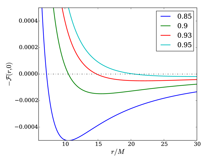
Figure 1: Plots of -$\mathcal{F}(r,0)$ for various values of $\lambda$ shown in the legend. The location where $\mathcal{F}(r,0)=0$ shows the radius of the ECS. -$\mathcal{F}(r,0)$ shows the forces acting on a stationary fluid, and so one can see how atmospheres can be constructed around the ECS.

We note the location of the ECS to be where $\mathcal{F}(r_{0},0)=0$, this gives

$$r_{0}=\dfrac{2M}{1-\lambda^{2}}.$$ (13)

It is important to note that $r_{0}$ is extremely sensitive to $\lambda$ as $\lambda\rightarrow 1$. This is further illustrated in Fig. 2.

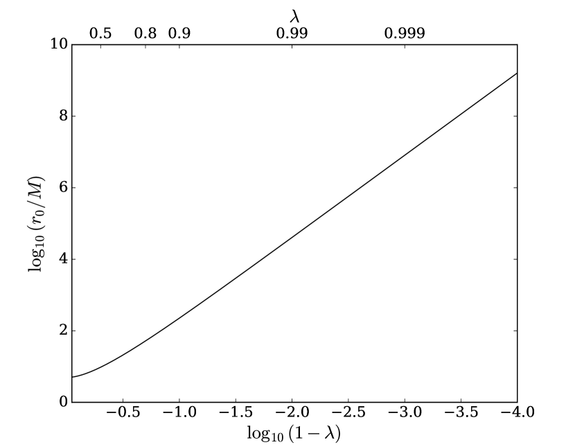
Figure 2: We have plotted $r_{0}$ as a function of $\lambda$. To illustrate the sensitivity of $r_{0}$ to $\lambda$, we have plotted against two different axis scales. The upper is $\lambda$ and the lower shows $\log(1-\lambda)$.

2.3 Atmospheric Solution

The equation for hydrostatic equilibrium, Eq. 5 was solved in Wielgus et al. (2015), who took an optically thin fluid at a sufficiently low temperature such that $\rho\gg p+u$, and derived atmospheric solutions with their pressure maximum located at radius $r_{0}$. They have provided a set of polytropic atmosphere solutions with polytropic index, $\Gamma$, given by

$$\rho(r)=\rho_{0}\left[\ln(1-2M/r)^{-1/2}-\lambda(1-2M/r)^{-1/2}+\lambda\right]^{\frac{1}{\Gamma-1}}.$$ (14)

Such an atmosphere is entirely supported by radiation and there are regions between the atmosphere and the surface of the star with no gas at all.

3 Radial eigenmode of an incompressible thin shell

Now we turn from hydrostatic equilibrium to the time dependent equation, the relativistic Euler equation, with which we will apply perturbations to derive the oscillation frequency. While we are in the relativistic regime of strong gravity, we will make the assumption that our velocities are small and so non-relativistic. This allows us to write the four velocity, $u^{\mu}$, to first order in $u^{r}=dr/d\tau$, or in $v=dr/dt$.

$$u^{\mu}=(u^{t},u^{r},0,0)=u^{t}(1,v,0,0)\approx\dfrac{1}{\sqrt{1-2M/r}}(1,v,0,0).$$ (15)

This allows us to simplify Eq. 3 to get,

$$\dfrac{d}{d\tau}u^{r}+\dfrac{1}{\rho}\left(g^{rr}\dfrac{\partial p}{\partial r}+u^{r}\dfrac{dp}{d\tau}\right)=-M\left(\dfrac{1}{r^{2}}-\dfrac{f^{r}}{M}\right)=-M\mathcal{F}(r,u^{r}),$$ (16)

We have combined the two non-fluid forces into one expression, $\mathcal{F}$, which is in general a function of $r$ and $u^{r}$. We will demonstrate that $\mathcal{F}$ can be divided into the sum of two terms, one of which is only a function of $r$, the other a function of both $r$ and $u^{r}$. The former corresponds to the radiation force, and the latter to radiation drag, both of which will play an important role in our analysis.

We let Eq. 5 serve as the background over which we consider spherically symmetric radial perturbations. In this work, we will consider an incompressible mode, where the whole atmosphere is transported by a small radial distance, $\xi$, while preserving its pressure and density profiles, $p(r)\rightarrow p_{b}(r-\xi)$, and $\rho(r)\rightarrow\rho_{b}(r-\xi)$, where the $b$ index indicates the background solutions. We also have, $u^{r}=d\xi/d\tau$. We will demonstrate that for a sufficiently thin atmosphere, we will recover a radial eigenmode that oscillates with the same frequency as a test particle about $r_{0}$. This gives us the following two equations to solve,

$$\dfrac{d^{2}\xi}{d\tau^{2}}+\dfrac{g^{rr}(r)}{\rho_{b}(r-\xi)}\left(\dfrac{\partial}{\partial r}p_{b}(r-\xi)\right) =-M\mathcal{F}(r,u^{r}),$$ (17)

$$\dfrac{g^{rr}(r)}{\rho_{b}(r)}\dfrac{\partial p_{b}(r)}{\partial r} =-M\mathcal{F}(r,0),$$ (18)

where we have been explicit with the $r$ dependence for clarity. The system can be simplified to one equation after expanding in terms of $\xi$, and substituting Eq. 18 into Eq. 17 to get,

$$\dfrac{1}{M}\dfrac{d^{2}\xi}{d\tau^{2}}-\mathcal{F}(r,0)+\dfrac{\partial\mathcal{F}(r,0)}{\partial r}\xi-\mathcal{F}(r,0)\dfrac{\partial\ln g^{rr}(r)}{\partial r}\xi=-\mathcal{F}(r,u^{r}).$$ (19)

At this point we invoke the thin shell limit. We assume that we have a thin atmosphere concentrated around, $r_{0}$. Also note that, $\mathcal{F}(r_{0},0)=0$, which we derived in the previous section. This allows us to expand $\mathcal{F}$ around $r=r_{0}$ and $u^{r}=0$ to get,

$$\mathcal{F}(r,u^{r})\approx(r-r_{0})\left.\dfrac{\partial\mathcal{F}}{\partial r}\right|_{r_{0},0}+u^{r}\left.\dfrac{\partial\mathcal{F}}{\partial u^{r}}\right|_{r_{0},0}.$$ (20)

Substituting in the expansion and noting that $\xi\cdot(r-r_{0})$ is second order in small quantities, we are left with the following equation,

$$\dfrac{1}{M}\dfrac{d^{2}\xi}{d\tau^{2}}+\left.\dfrac{\partial\mathcal{F}}{\partial u^{r}}\right|_{r_{0},0}\dfrac{d\xi}{d\tau}+\left.\dfrac{\partial\mathcal{F}}{\partial r}\right|_{r_{0},0}\xi=0.$$ (21)

This is the equation for a damped harmonic oscillator (assuming the appropriate signs for the derivatives of $\mathcal{F}$). The equation of motion contains no fluid terms and so we expect this particular incompressible mode to oscillate about the equilibrium position with the same frequency as a test particle, in fact, the trajectories should be identical in the limit of small perturbations.

4 Oscillations

4.1 Undamped Oscillation Frequency

Our equation of motion in the thin shell limit is given by Eq. 21. In order to calculate the frequency of oscillations, first we will neglect the damping (second) term in Eq. 21.

If

$$\left.\dfrac{\partial\mathcal{F}}{\partial r}\right|_{r_{0},0}>0,$$ (22)

then we can expect the harmonic oscillator solution, with angular frequency,

$$\tilde{\omega}=\sqrt{M\left.\dfrac{\partial\mathcal{F}}{\partial r}\right|_{r_{0},0}}.$$ (23)

We can tell this is true from Fig. 1, but we will calculate it explicitly to find the frequency that the atmosphere would oscillate at if the radiation drag were negligible.

Taking the derivative and substituting for the radius of the equilibrium position in terms of $\lambda$ we get

$$\tilde{\omega}=\dfrac{(1-\lambda^{2})^{2}}{4M\lambda}.$$ (24)

To put our angular frequency in terms of s^-1 we restore $c$ and $G$ to get $\omega=c^{3}\tilde{\omega}/G$.

We have calculated our angular frequency with respect to the proper time experienced by the shell, $\tau$, so we multiply by a factor of $g_{tt}$ to redshift the angular frequency into the coordinate time, $t$. $\omega^{\prime}=\omega\sqrt{1-2M/r_{0}}=\lambda\omega$. The frequency, $\nu=\omega^{\prime}/2\pi$, is then

$$\nu=\dfrac{c^{3}}{2\pi G}\lambda\tilde{\omega}\approx 8.08(1-\lambda^{2})^{2}\dfrac{M_{\odot}}{M}\,\text{kHz}.$$ (25)

In Fig. 3 we can see a plot of $\nu$ as a function of $\lambda$. An example value of $\lambda=0.8$ with a mass of $1.4M_{\odot}$ gives, $\nu=750$ Hz.

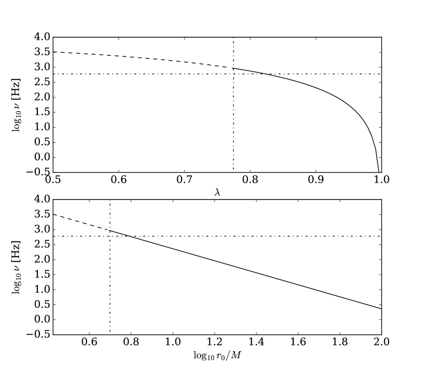
Figure 3: A plot of frequency of oscillations, $\nu$, about $r_{0}$ with respect to the Eddington ratio, $\lambda$, above, and with respect to $r_{0}$ below. Also shown is the interesting frequency, 600 Hz which corresponds to $\lambda\sim 0.82$ and the $\lambda$ for which $r_{0}=5M$, below which the frequency is not physical.

4.2 Damped Oscillations

At this point we calculate the strength of the radiation drag for small velocities. If the drag coefficient is small then we should further explore this and other oscillation modes as a possible explanation for X-ray burst QPOs. If we find that the drag coefficient is large enough to overdamp the oscillations, then we should rule out this particular mode of the optically thin atmospheres. Although, one should still study the oscillatory behavior of the optically thick atmospheres which may be different.

Our equation of motion is now given by

$$\dfrac{1}{M}\dfrac{d^{2}\xi}{d\tau^{2}}+\left.\dfrac{\partial\mathcal{F}}{\partial u^{r}}\right|_{r_{0},0}\dfrac{d\xi}{d\tau}+\dfrac{(1-\lambda^{2})^{4}}{16M^{3}\lambda^{2}}\xi=0.$$ (26)

To calculate the drag coefficient for our linearized equation of motion, we just need to evaluate the $u^{r}$ derivative of $\mathcal{F}$.

To calculate the $u^{r}$ derivative, we return to our equation for the flux, where we have already simplified the first term. Substituting for $I(r)$ gives

$$F^{r}=\dfrac{L_{\infty}}{4\pi r^{2}}-\dfrac{L_{\infty}}{4\pi R^{2}}\dfrac{1-2M/R}{(1-2M/r)^{2}}\left[\tilde{T}^{(r)(r)}+\tilde{\epsilon}\right]u^{r}.$$ (27)

We take the definition of $\tilde{\epsilon}$ from Stahl et al. (2013),

$$\tilde{\epsilon}=\dfrac{T^{\mu\nu}u_{\mu}u_{\nu}}{\pi I(r)},$$ (28)

and the relevant, dimensionless tetrad components of $T^{\mu\nu}$ written as, $\tilde{T}^{(t)(t)}$ and $\tilde{T}^{(r)(r)}$, derived in Abramowicz et al. (1990), given by

$$\tilde{T}^{(t)(t)} =2(1-\cos\alpha(r)),$$ (29)

$$\tilde{T}^{(r)(r)} =\dfrac{2}{3}(1-\cos^{3}\alpha(r)),$$ (30)

also in terms of the viewing angle, $\alpha(r)$. Substituting back into the equation of motion keeping terms to 1st order in $u^{r}$, we now have

$$\mathcal{F}(r,u^{r})=\dfrac{1}{r^{2}}-\dfrac{\lambda}{r^{2}\sqrt{1-2M/r}}+\dfrac{1}{R^{2}}\dfrac{1-2M/R}{(1-2M/r)^{2}}\left[\tilde{T}^{(r)(r)}+\tilde{T}^{(t)(t)}\right]u^{r},$$ (31)

which makes evaluating the derivative very simple,

$$\dfrac{\partial\mathcal{F}}{\partial u^{r}}=\dfrac{\lambda}{R^{2}}\dfrac{1-2M/R}{(1-2M/r)^{2}}\left[\tilde{T}^{(r)(r)}+\tilde{T}^{(t)(t)}\right].$$ (32)

At the point we only need to evaluate the derivative at $r_{0}$,

$$\left.\dfrac{\partial\mathcal{F}}{\partial u^{r}}\right|_{r_{0},0}=\dfrac{1-2M/R}{\lambda^{3}R^{2}}\left[\frac{2}{3}(1-\cos\alpha_{0})\left(\cos^{2}\alpha_{0}+\cos\alpha_{0}+4\right)\right],$$ (33)

where

$$\sin^{2}\alpha(r_{0})=(1-\lambda^{2})^{2}\dfrac{\lambda^{2}}{4}\dfrac{(R/M)^{2}}{1-2M/R}.$$ (34)

From here, it becomes much simpler to switch to dimensionless variables scaled by the neutron star mass,

$$\dfrac{r}{M}\rightarrow x$$

$$\dfrac{R}{M}\rightarrow X$$

$$\dfrac{\xi}{M}\rightarrow\tilde{\xi}$$

$$\dfrac{\tau}{M}\rightarrow\tilde{\tau}$$

Then the equation of motion is

$$\dfrac{d^{2}\tilde{\xi}}{d\tilde{\tau}^{2}}+M^{2}\left.\dfrac{\partial\mathcal{F}}{\partial u^{r}}\right|_{r_{0},0}\dfrac{d\tilde{\xi}}{d\tilde{\tau}}+\left.\dfrac{\partial\mathcal{F}}{\partial r}\right|_{r_{0},0}M^{3}\tilde{\xi}=0.$$ (35)

If, for convenience, we set the dimensionless quantities

$$f =M^{3}\left.\dfrac{\partial\mathcal{F}}{\partial r}\right|_{r_{0},0}=\dfrac{(1-\lambda^{2})^{4}}{16\lambda^{2}},$$ (36)

$$g =M^{2}\left.\dfrac{\partial\mathcal{F}}{\partial u^{r}}\right|_{r_{0},0}=\dfrac{1-2/X}{\lambda^{3}X^{2}}\left[\frac{2}{3}(1-\cos\alpha_{0})\left(\cos^{2}\alpha_{0}+\cos\alpha_{0}+4\right)\right],$$ (37)

then we can classify the damping from the sign of

$$\tilde{\omega}_{d}^{2}=\dfrac{g^{2}}{4}-f.$$ (38)

If $\omega_{d}^{2}<0$ then we have an underdamped oscillation, $\omega_{d}^{2}>0$ is overdamped and $\omega_{d}=0$ is critically damped.

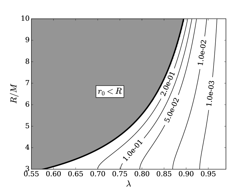
Figure 4: Contours of $\tilde{\omega}_{d}^{2}/\tilde{\omega}^{2}$ over a reasonable parameter space for neutron star radius, $R$, and Eddington ratio, $\lambda$. The grey region on the left side of the plot corresponds to $r_{0}<R$ which is unphysical. The thick line marks the boundary where $r_{0}=R$. There is no region on the plot where $\tilde{\omega_{d}}^{2}$ is less than zero which means that the thin shell eigenmode is overdamped over the parameter space we consider.

If we take some example values as before, $\lambda=0.8$ and $R=5M$, then we get

$$f\approx 0.0016,g\approx 0.089,$$

$$\omega_{d}\approx 0.06=885\,\text{s}^{-1}.$$

Because $\omega_{d}$ is real, we have an overdamped solution with an exponential decay without oscillation. For this reason we do not label non-oscillating quantities of dimension $[s]^{-1}$ with Hz, so that they are not to be thought of as oscillation frequencies, but rather inverse decay timescales. In fact, over the whole reasonable parameter space of $\lambda$ and $R$, the eigenmode is overdamped. This can be seen in Fig. 4, a plot of the ratio of $\tilde{\omega}_{d}^{2}$ to $\tilde{\omega}^{2}$. We can see that for small $\lambda$ we are strongly overdamped and as $\lambda$ increases the solution approaches critical damping. Our damped harmonic oscillator equation yields two exponential solutions of the form $C_{\pm}\exp(\gamma_{\pm}\tau)$. where

$$\gamma_{\pm}=-\dfrac{g}{2}\pm\sqrt{\dfrac{g^{2}}{4}-f}.$$ (39)

Both of which correspond to decay constants of $\gamma_{+}=-0.025,\gamma_{-}=-0.064$. If we convert to seconds and redshift for the observer at infinity we have

$$\gamma_{\pm}^{\prime}=\dfrac{c\sqrt{B(r_{0})}}{2\pi r_{g}}\gamma_{\pm}=32.31\times 10^{3}\,\text{s}^{-1}\,\left(\dfrac{M}{M_{\odot}}\right)^{-1}\lambda\gamma_{\pm},$$ (40)

$$\gamma_{+}^{\prime}=369\,\text{s}^{-1},\gamma_{-}=945\,\text{s}^{-1}.$$

The scales of decay for each solution are then $1/\gamma_{\pm}$ so

$$\tau_{+}=0.0027\,\text{s},\tau_{-}=0.0011\,\text{s}.$$

5 Validity of the nonlinear regime

A key assumption mentioned at the beginning of the work relied on the atmosphere’s thickness and velocities being small enough to be able to linearize $\mathcal{F}(r,u^{r})$. This allows us to obtain analytical trajectories for the fluid for the thin shell mode, but we are interested to see the extent to which this linearisation is valid, both in position and velocity. While we do not expect oscillatory behavior to exist at larger velocities and displacements, we can still study how the timescale for decay varies from that predicted by the analytical treatment.

To explore the degree to which the linear regime of $\mathcal{F}$ is valid we compare the trajectories of the thin shell mode to those of test particles which obey the equation of motion,

$$\dfrac{d^{2}\tilde{\xi}}{d\tilde{\tau}^{2}}=-M^{2}\mathcal{F}(r,u^{t}).$$ (41)

We expect the trajectories from this equation, given by $\xi_{e}(t)$ to be similar to the trajectories given by Eq. 21, which we will denote, $\xi_{a}(t)$.

To integrate this equation we use the odeint routine from the scipy package which relies on the lsoda routine from the FORTRAN library odepack. We test a variety of initial conditions. We plot these against the analytical trajectories given by solving the linear equation of motion, of which the trajectories are just linear combinations of exponentials. The plots, shown in Fig. 5, show both trajectories from the linear equation of motion (blue) and from the full equation of motion (red dashed).

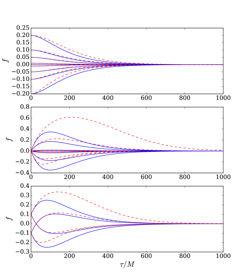
Figure 5: Trajectories from a variety of initial conditions analytically integrated from the linearized equation of motion, Eq. 21 (blue), and numerically integrated from the test particle equation of motion, Eq. 41 (red dashed). The vertical axes show, $f$, the fraction the initial position is from the ECS. Upper: The initial velocity is zero and the initial position can be read from the axis. Middle: The initial position is at the ECS and the initial velocities are given by, $v(0)/c=\pm 0.005,\pm 0.01,\pm 0.05,\pm 0.1$. Lower: Initial conditions are given by $(f(0),v(0)/c)=(0.1,0.05),(0.1,-0.05),(-0.1,0.05),(-.1,-0.05).$

The first plot in Fig. 5 shows trajectories starting with zero initial velocity. The initial positions of the test particle are readable form the axis where the y-axis represents the fractional displacement from the equilibrium position $f=(r(0)-r_{0})/r_{0}$. We can see from the plot that deviations from the test particle solution start to occur between $f=0.1$ and $f=0.2$. The deviation is small however and the atmosphere settles into the equilibrium position at about the same time as the test particle. We expect that for $v(0)=0$, the atmosphere trajectory is valid up to initial displacements of $10\%$ from the equilibrium solution, and a reasonable approximation up to $20\%$ away.

The second plot in Fig. 5 shows trajectories with an initial position at the equilibrium position, but with different initial velocities of $v(0)/c=\pm 0.005,\pm 0.01,\pm 0.05,\pm 0.1$. We can immediately see that $v(0)=\pm 0.1c$ shows vastly different trajectories, which are also highly asymmetrical with respect to the equilibrium position, indicating that the atmospheric approximation is no longer valid and even at $v(0)/c=\pm 0.5$ there are significant deviations. We expect the linear regime in this case to hold up to $v(0)/c=\pm 0.01$.

The third plot in Fig. 5 shows trajectories corresponding to the following initial conditions:

$$(f(0),v(0)/c)=(0.1,0.05),(0.1,-0.05),(-0.1,0.05),(-.1,-0.05).$$

The two inner trajectories show much better agreement with the test particle. This is because their initial conditions keep them closer to the equilibrium position where the atmospheric equation of motion more accurately reflects that of the test particle.

5.1 Convergence

We also find it necessary to numerically confirm the convergence of the linearised fluid equation to the test particle equation. In essence, we want to show that the trajectories from the Eq. 21 approach those from Eq. 41 as $\xi(0)\rightarrow 0,u^{r}(0)\rightarrow 0$. We measure the deviation in the trajectory by summing up the fractional difference along $n=100$ points, denoted by $\tau_{i}$, which are evenly sampled along the trajectories shown in Fig. 5. The error per time step is then calculated by,

$$\epsilon=\dfrac{1}{n}\sum_{i=0}^{n}\dfrac{\left|\xi_{e}(\tau_{i})-\xi_{a}(\tau_{i})\right|}{\xi_{e}(\tau_{i})},$$ (42)

which we calculate for different values of the initial conditions, $(\xi(0),u^{r}(0))=(\delta_{1},\delta_{2})$. A plot of the convergence is shown in Fig. 6. We can see that $\epsilon$ shrinks to the level of machine precision as $\delta_{1},\delta_{2}$ approach zero.

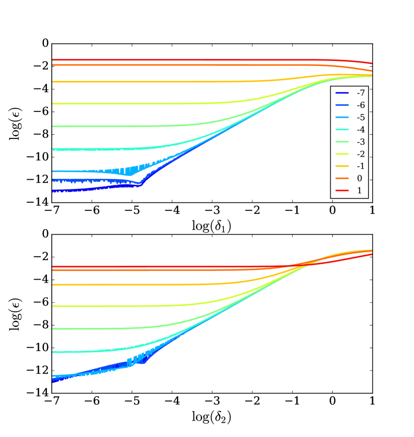
Figure 6: Here we show the results of the convergence test for the linearisation of the equation of motion. For initial conditions $(\xi(0),u^{r}(0))=(\delta_{1},\delta_{2})$. The upper panel shows different curves corresponding to different $\delta_{2}$ as indicated by the legend. The $\delta_{1}$s are shown on the horizontal axis. The lower plot shows the same except for different curves of $\delta_{1}$ with $\delta_{2}$ on the horizontal axis.

6 Discussion and Conclusions

6.1 Consequences for the stability of atmospheres

We have shown that for optically thin levitating atmospheres, as in Wielgus et al. (2015), the radial, incompressible, thin shell modes are stable against radial oscillations due to the strength of the radiation drag term. The natural frequency of these oscillations is on the order of $\sim 10^{2}$ Hz if they were not overdamped. Moreover the frequency increases as the luminosity decreases. This would lead to an increase of frequency with time if the luminosity were to decay with time, such as during the decay phase of an X-ray burst. These oscillations are exactly the same as test particle oscillations, and the incompressible mode is constructed in a way that does not allow for extra forces due to pressure gradients. It is possible to conceive of a mode where the pressure terms become important, such as a breathing mode where the shell expands and contracts in opposite directions about the pressure maximum so that the shell becomes thinner and thicker. It is also possible to construct pressure corrections to the thin shell incompressible mode to extend its validity to larger thicknesses. If the eigenfrequency of such a mode is large enough, one can imagine that underdamped oscillations may occur, and so it would be worth exploring such other modes.

6.2 Optically Thick Oscillations

In this work we have only considered optically thin solutions. Wielgus et al. (2016) have extended their work to include optically thick atmospheres. These atmospheres are constructed using numerical techniques, so it is difficult to calculate analytical oscillation modes. In future work, we plan to extend this analysis to include numerical simulations of both optically thin and thick Eddington supported atmospheres. Since photons diffuse through the optically thick atmospheres, as opposed to free streaming through the thin ones, it is possible that the radiation drag is less efficient at damping oscillations. We except the drag to only be effective in the optically thin edges of the atmospheres.

7 acknowledgements

The authors thank Maciek Wielgus and Omer Blaes for useful discussions during the work. The research was supported by the Polish NCN grant 2013/08/A/ST9/00795.

References

- Abramowicz et al. (1990) Abramowicz, M. A., Ellis, G. F. R., & Lanza, A. 1990, ApJ, 361, 470
- Bachetti et al. (2014) Bachetti, M., Harrison, F. A., Walton, D. J., et al. 2014, Nature, 514, 202
- Phinney (1987) Phinney, E. S. 1987, Superluminal Radio Sources, 301
- Remillard & McClintock (2006) Remillard, R. A., & McClintock, J. E. 2006, ARA&A, 44, 49
- Stahl et al. (2012) Stahl, A., Wielgus, M., Abramowicz, M., Kluźniak, W., & Yu, W. 2012, A&A, 546, A54
- Stahl et al. (2013) Stahl, A., Kluźniak, W., Wielgus, M., & Abramowicz, M. 2013, A&A, 555, A114
- Strohmayer (1999) Strohmayer, T. E. 1999, arXiv:astro-ph/9911338
- Strohmayer & Bildsten (2006) Strohmayer, T., & Bildsten, L. 2006, Compact stellar X-ray sources, 39, 113
- van der Klis (2006) van der Klis, M. 2006, Compact stellar X-ray sources, 39, 39
- Wielgus et al. (2012) Wielgus, M., Stahl, A., Abramowicz, M., & Kluźniak, W. 2012, A&A, 545, A123
- Wielgus et al. (2015) Wielgus, M., Kluźniak, W., Sa̧dowski, A., Narayan, R., & Abramowicz, M. 2015, MNRAS, 454, 3766
- Wielgus et al. (2016) Wielgus, M., Sa̧dowski, A., Kluźniak, W., Abramowicz, M., & Narayan, R. 2016, MNRAS, 458, 3420