On the numerical quadrature of weakly singular oscillatory integral and its fast implementation

Abstract

In this paper, we present a Clenshaw–Curtis–Filon–type method for the weakly singular oscillatory integral with Fourier and Hankel kernels. By interpolating the non-oscillatory and nonsingular part of the integrand at $(N+1)$ Clenshaw–Curtis points, the method can be implemented in $O(N\log N)$ operations. The method requires the accurate computation of modified moments. We first give a method for the derivation of the recurrence relation for the modified moments, which can be applied to the derivation of the recurrence relation for the modified moments corresponding to other type oscillatory integrals. By using recurrence relation, special functions and classic quadrature methods, the modified moments can be computed accurately and efficiently. Then, we present the corresponding error bound in inverse powers of frequencies $k$ and $\omega$ for the proposed method. Numerical examples are provided to support the theoretical results and show the efficiency and accuracy of the method.

1 Introduction

In this work we consider the evaluation of the weakly singular oscillatory integral of the form

$$I[f]=\int_{0}^{1}f(x)x^{\alpha}(1-x)^{\beta}\mathrm{e}^{\mathrm{i}2kx}H_{\nu}^{(1)}(\omega x)\,\mathrm{d}x$$ (1.1)

where $\alpha-|\nu|>-1,\beta>-1$, and $k\gg 1,\omega\gg 1$, $H^{(1)}_{\nu}(x)=J_{\nu}(x)+\mathrm{i}Y_{\nu}(x)$ is Hankel function of the first kind of order $\nu$, and $f$ is a sufficiently smooth function on $[0,1]$. In many areas of science and engineering, for example, in astronomy, optics, quantum mechanics, seismology image processing, electromagnetic scattering ([2], [3], [4], [11], [21]), one will come across the computation of the integral (1.1).

The integral (1.1) has the following two characteristics:

1. When $k+\omega\gg 1$, the integrand becomes highly oscillatory. Consequently, a prohibitively number of quadrature nodes are needed to obtain satisfied accuracy if one uses classical numerical methods like Simpson rule, Gaussian quadrature, etc. Moreover, it presents serious difficulties in obtaining numerical convergence of the integration.

2. The function $H_{\nu}^{(1)}(x)$ has a logarithmic singularity for $\nu=0$, and algebraic singularity for $\nu\neq 0$ at the point $x$=0. In addition, if $-1<\alpha,\beta<0$, the integrand also has algebraic singularities at two endpoints, which impacts heavily on its quadrature and its error bound. For a special case that $\alpha=0,\beta=0$, and $k=0$, the integral can be rewritten in a special form

   $$I[f]=\int_{0}^{1}f(x)H_{\nu}^{(1)}(\omega x)\,\mathrm{d}x.$$ (1.2)

In the last few years, many efficient numerical methods has been devised for the evaluation of oscillatory integrals. Here, we only mention several main methods, such as Levin method and Levin-type method [28, 29, 35], generalized quadrature rule [15, 16], Filon method and Filon–type method [12, 13, 17, 23, 40, 41, 42], Gauss–Laguerre quadrature [7, 8, 10, 21, 22, 23, 44]. In what follows, we will introduce several other papers related to the integrals considered in this paper. For the integral $\int_{0}^{1}f(x)x^{\alpha}(1-x)^{\beta}\mathrm{e}^{\mathrm{i}kx}\,\mathrm{d}x$, as early as in 1992, Piessens [37] construct a fast algorithm to approximate it by truncating $f$ by its Chebyshev series and using the recurrence relation of the modified moments. Recently, the references [24, 25] developed this method by using a special Hermite interpolation at Clenshaw–Crutis points and Chebyshev expansion for $\mathrm{e}^{\mathrm{i}kx}$. If $f$ is analytic in a sufficiently large complex region containing $[0,1]$, a numerical steepest descent method [26] was presented by using complex integration theory. The same idea is also applied to the the computation of the integral $\int_{a}^{b}(x-a)^{\alpha}(b-x)^{\beta}\ln(x-a)f(x)\mathrm{e}^{\mathrm{i}\omega x}\,\mathrm{d}x,\alpha,\beta>-1$, based on construction of the Gauss quadrature rule with logarithmic weight function [18]. For the integral $\int_{0}^{1}f(x)x^{\alpha}(1-x)^{\beta}J_{m}(\omega x)\,\mathrm{d}x,\alpha,\beta>-1$, a Filon-type method based on a special Hermite interpolation polynomial at Clenshaw–Curtis points was introduced in [9]. On the other hand, the reference [27] proposed a Clenshaw–Curtis–Filon method for the computation of the oscillatory Bessel integral $\int_{0}^{1}f(x)x^{\alpha}\ln(x)(1-x)^{\beta}J_{m}(\omega x)\,\mathrm{d}x,\alpha,\beta>-1$, with algebraic or logarithmic singularities at the two endpoints.

For the evaluation of the integral (1.1), the literature [18] transformed it into two line integrals by using the analytic continuation and the construction of Gauss quadrature rules. However, this method require that $f$ is analytic in a enough large region. A recent work [45] present a Clenshaw–Curtis–Filon–type method for the special case $\alpha=\beta=k=0$ by using special functions. In addition, a composite method [13] can also be applied to the computation of this integral for this case, by absorbing the non-oscillatory part of Hankel function into $f$, then interpolating its product with $f$. However, as the author in [45] pointed out that the accuracy of this method may becomes worse as the number of Clenshaw–Curtis points increases and the fastest convergence of this method obtained is $O(\omega^{-2})$ for fixed number of Clenshaw–Curtis points.

In view of the advantages of Clenshaw–Curtis–Filon method, in this paper we will consider a higher order Clenshaw–Curtis–Filon–type method for the integral (1.1), which does not require that $f$ is analytic in a enough large region. As we know, the fast implementation of Clenshaw–Curtis–Filon method largely depends on the accurate and efficient computation of modified moments. In addition, the key problem of the efficient computation of the modified moments is the how to obtain the recurrence relation for them. Fortunately, we can give a universal method for the derivation of the recurrence relation for the modified moments. Moreover, this method can be applied to the modified moments with other type kernels.

The outline of this paper is organized as follows. In Section 2, we describe the Clenshaw–Curtis–Filon–type for the integral (1.1), and present a universal method for the derivation of the recurrence relation for the modified moments, by which the modified moments can be efficiently computed with several initial values. In Section 3, we give an error bound on $k$ and $\omega$ for the presented method. Some examples are given in Section 4 to show the efficiency and accuracy. Finally, we finish this paper in Section 5 by presenting some concluding remarks.

2 Clenshaw–Curtis–Filon–type method and its implementation

In what follows we will consider a Clenshaw–Curtis–Filon–type method for the integrals (1.1) and its fast implementation. Suppose that $f$ is a sufficiently function on $[0,1]$, and let $P_{N+2s}(x)$ denote the Hermite interpolation polynomial at the Clenshaw–Curtis points

$$x_{j}=\big{(}1+\cos(j\pi/N)\big{)}/2,\ j=0,\ldots,N,$$

where $s$ is a nonnegative integer, and for $\ell=0,\ldots,s$, there holds

$$P_{N+2s}^{(\ell)}(0)=f^{(\ell)}(0),\textrm{\quad}P_{N+2s}(x_{j})=f(x_{j}),\textrm{\quad}P_{N+2s}^{(\ell)}(1)=f^{(\ell)}(1),\textrm{\quad}j=1,\ldots,N-1.$$ (2.1)

Then $P_{N+2s}(x)$ can be written in the following form

$$P_{N+2s}(x)=\sum_{n=0}^{N+2s}a_{n}T^{\ast}_{n}(x),$$ (2.2)

where $a_{n}$ can be fast calculated by fast Fourier transform [40] with $O(N\log N)$ operations, $T^{\ast}_{n}(x)$ is the shifted Chebyshev polynomial of the first kind of degree $n$ on $[0,1]$.

In view of (2.1) and (2.2), we can define Clenshaw–Curtis–Filon–type method for the integral (1.1) by

$$Q_{N,s}^{CCF}[f]=\int_{0}^{1}P_{N+2s}(x)x^{\alpha}(1-x)^{\beta}\mathrm{e}^{\mathrm{i}2kx}H_{\nu}^{(1)}(\omega x)\,\mathrm{d}x=\sum_{n=0}^{N+2s}a_{n}M(n,k,\omega),$$ (2.3)

where the modified moments

$$M(n,k,\omega)=\int_{0}^{1}x^{\alpha}(1-x)^{\beta}T^{\ast}_{n}(x)\mathrm{e}^{\mathrm{i}2kx}H_{\nu}^{(1)}(\omega x)\,\mathrm{d}x$$ (2.4)

have to be computed accurately.

2.1 Recurrence relation for the modified moments

As we have stated in Section 1, the key problem of the fast computations of the modified moment $M(n,k,\omega)$ is to obtain a recurrence relation for them. In the following, we will give a universal method for the derivation of the recurrence relation for the modified moments.

Theorem 2.1

The modified moments $M(n,k,\omega)$ for $n\geq 4,k\geq 0,\omega>0$ satisfy the following recurrence relation:

$$\Big{(}\frac{1}{16}\omega^{2}-\frac{1}{4}k^{2}\Big{)}M(n+4,k,\omega)+f_{1}(n,\alpha,\beta)M(n+3,k,\omega)+f_{2}(n,\alpha,\beta)M(n+2,k,\omega)$$

$$+f_{3}(n,\alpha,\beta)M(n+1,k,\omega)+f_{4}(n,\alpha,\beta)M(n,k,\omega)+f_{3}(-n,\alpha,\beta)M(n-1,k,\omega)$$

$$+f_{2}(-n,\alpha,\beta)M(n-2,k,\omega)+f_{1}(-n,\alpha,\beta)M(n-3,k,\omega)$$

$$+\Big{(}\frac{1}{16}\omega^{2}-\frac{1}{4}k^{2}\Big{)}M(n-4,k,\omega)=0,$$ (2.5)

where

$$f_{1}(n,\alpha,\beta)= \mathrm{i}k(\alpha+\beta+n+4)-\frac{1}{2}\mathrm{i}k,$$ (2.6)

$$f_{2}(n,\alpha,\beta)= 9+6(\alpha+\beta+n)+k^{2}+n^{2}+\alpha^{2}+\beta^{2}-\frac{1}{4}\omega^{2}-\nu^{2}$$

$$+2(\alpha\beta+\alpha n+\beta n)+\mathrm{i}k(1-2\alpha+2\beta),$$ (2.7)

$$f_{3}(n,\alpha,\beta)= 2n-8\alpha+12\beta+4(1-\mathrm{i}\alpha k-\mathrm{i}\beta k+\nu^{2}+\beta n-\alpha n)$$

$$-\frac{31}{2}\mathrm{i}k+3\mathrm{i}k(\alpha+\beta-n+4)+4(\beta^{2}-\alpha^{2}),$$ (2.8)

$$f_{4}(n,\alpha,\beta)= 6+4\alpha+12\beta-4\alpha\beta-2\mathrm{i}k+4\mathrm{i}k(\alpha-\beta)$$

$$+\frac{3}{8}\omega^{2}-\frac{3}{2}k^{2}+6(\alpha^{2}+\beta^{2}-\nu^{2})-2n^{2}.$$ (2.9)

Proof: First, we can rewrite the modified moments $M(n,k,\omega)$ by

$$M(n,k,\omega)=\frac{1}{2^{\alpha+\beta+1}}\mathrm{e}^{\mathrm{i}k}\int_{-1}^{1}(1+x)^{\alpha}(1-x)^{\beta}T_{n}(x)\mathrm{e}^{\mathrm{i}kx}H_{\nu}^{(1)}\big{(}\frac{1+x}{2}\omega\big{)}\,\mathrm{d}x,$$ (2.10)

where $T_{n}(x)$ is the Chebyshev polynomial of degree $n$ of the first kind.

Form the above equality, we can see that the modified moments $M(n,k,\omega)$ and the integral $\int_{-1}^{1}(1+x)^{\alpha}(1-x)^{\beta}T_{n}(x)\mathrm{e}^{\mathrm{i}kx}H_{\nu}^{(1)}\big{(}\frac{1+x}{2}\omega\big{)}\,\mathrm{d}x$ have the same recurrence relation.

Since the function $y=H_{\nu}^{(1)}(x)$ satisfies the following Bessel’s differential equation [1, p. 358]

$$x^{2}\frac{d^{2}y}{\,\mathrm{d}x^{2}}+x\frac{dy}{\,\mathrm{d}x}+(x^{2}-\nu^{2})=0,$$ (2.11)

we have

$$(1+x)^{2}\Big{[}H_{\nu}^{(1)}\big{(}\frac{1+x}{2}\omega\big{)}\Big{]}^{\prime\prime}+(1+x)\Big{[}H_{\nu}^{(1)}\big{(}\frac{1+x}{2}\omega\big{)}\Big{]}^{\prime}$$

$$-\Big{(}\nu^{2}-\frac{(1+x)^{2}\omega^{2}}{4}\Big{)}H_{\nu}^{(1)}\big{(}\frac{1+x}{2}\omega\big{)}=0.$$ (2.12)

Let

$$K_{1}=4\int_{-1}^{1}(1+x)^{\alpha}(1-x)^{\beta}(1-x)^{2}(1+x)^{2}\mathrm{e}^{\mathrm{i}kx}\Big{[}H_{\nu}^{(1)}\big{(}\frac{1+x}{2}\omega\big{)}\Big{]}^{\prime\prime}T_{n}(x)\,\mathrm{d}x,$$ (2.13)

$$K_{2}=4\int_{-1}^{1}(1+x)^{\alpha}(1-x)^{\beta}(1-x)^{2}(1+x)\mathrm{e}^{\mathrm{i}kx}\Big{[}H_{\nu}^{(1)}\big{(}\frac{1+x}{2}\omega\big{)}\Big{]}^{\prime}T_{n}(x)\,\mathrm{d}x,$$ (2.14)

and

$$K_{3}=4\int_{-1}^{1}(1+x)^{\alpha}(1-x)^{\beta}(1-x)^{2}\Big{(}\nu^{2}-\frac{(1+x)^{2}\omega^{2}}{4}\Big{)}\mathrm{e}^{\mathrm{i}kx}H_{\nu}^{(1)}\big{(}\frac{1+x}{2}\omega\big{)}T_{n}(x)\,\mathrm{d}x.$$ (2.15)

It follows from (2.1) that

$$K_{1}+K_{2}-K3=0.$$ (2.16)

Noting that the integrands in $K_{1}$ and $K_{2}$ have the common factor $(1-x)^{2}$ and using integration by parts, we can easily get

$$K_{1}=4\int_{-1}^{1}\big{[}(1+x)^{\alpha}(1-x)^{\beta}(1-x)^{2}(1+x)^{2}\mathrm{e}^{\mathrm{i}kx}T_{n}(x)\big{]}^{\prime\prime}H_{\nu}^{(1)}\big{(}\frac{1+x}{2}\omega\big{)}\,\mathrm{d}x,$$ (2.17)

$$K_{2}=4\int_{-1}^{1}\big{[}(1+x)^{\alpha}(1-x)^{\beta}(1-x)^{2}(1+x)\mathrm{e}^{\mathrm{i}kx}T_{n}(x)\big{]}^{\prime}H_{\nu}^{(1)}\big{(}\frac{1+x}{2}\omega\big{)}\,\mathrm{d}x.$$ (2.18)

According to the properties of the Chebyshev polynomial of the first kind[32]

$$x^{m}T_{n}(x)=2^{-m}\sum_{j=0}^{m}\binom{m}{j}T_{n+m-2j}(x),$$

and

$$\frac{d}{\,\mathrm{d}x}T_{n}(x)=\frac{n}{2}\frac{T_{n-1}(x)-T_{n+1}(x)}{1-x^{2}},$$

by rewriting the integrands in $K_{1},K_{2}$ and $K_{3}$ as the sum of the product of Chebyshev polynomials of different degree and $(1+x)^{\alpha}(1-x)^{\beta}\mathrm{e}^{\mathrm{i}kx}H_{\nu}^{(1)}\big{(}\frac{1+x}{2}\omega\big{)}$, we derive

$$K_{1} = -\frac{1}{4}k^{2}M(n+4,k,\omega)+f_{5}(n,\alpha,\beta)M(n+3,k,\omega)+f_{6}(n,\alpha,\beta)M(n+2,k,\omega)$$ (2.19)

$$+f_{7}(n,\alpha,\beta)M(n+1,k,\omega)+f_{8}(n,\alpha,\beta)M(n,k,\omega)+f_{7}(-n,\alpha,\beta)M(n-1,k,\omega)$$

$$+f_{6}(-n,\alpha,\beta)M(n-2,k,\omega)+f_{5}(-n,\alpha,\beta)M(n-3,k,\omega)$$

$$-\frac{1}{4}k^{2}M(n-4,k,\omega),$$

where

$$f_{5}(n,\alpha,\beta) = \mathrm{i}k(\alpha+\beta+n+4),$$ (2.20)

$$f_{6}(n,\alpha,\beta) = 12+7(\alpha+\beta+n)+k^{2}+n^{2}+\alpha^{2}+\beta^{2}$$ (2.21)

$$+2(\alpha\beta+\alpha n+\beta n)+2\mathrm{i}k(\beta-\alpha),$$

$$f_{7}(n,\alpha,\beta) = 12(\beta-\alpha)-4\mathrm{i}k(\alpha+\beta)+4(\beta n-\alpha n)$$ (2.22)

$$+3\mathrm{i}k(\alpha+\beta-n+4)+4(\beta^{2}-\alpha^{2}),$$

$$f_{8}(n,\alpha,\beta) = 8+10(\alpha+\beta)+4\mathrm{i}k(\alpha-\beta)-2n^{2}-\frac{3}{2}k^{2}$$ (2.23)

$$+6(\alpha^{2}+\beta^{2})-4\alpha\beta,$$

$$K_{2} = -\bigg{\{}\frac{1}{2}\mathrm{i}kM(n+3,k,\omega)+(\alpha+\beta+n+3-\mathrm{i}k)M(n+2,k,\omega)$$ (2.24)

$$-(\frac{1}{2}\mathrm{i}k+4+4\alpha+2n)M(n+1,k,\omega)+(6\alpha-2\beta+2\mathrm{i}k+2)M(n,k,\omega)$$

$$-(\frac{1}{2}\mathrm{i}k+4+4\alpha+2n)M(n-1,k,\omega)+(\alpha+\beta-n+3-\mathrm{i}k)M(n-2,k,\omega)$$

$$+\frac{1}{2}\mathrm{i}kM(n-3,k,\omega)\bigg{\}},$$

$$K_{3} = -\frac{1}{16}\bigg{\{}\omega^{2}M(n+4,k,\omega)-(4\omega^{2}+16\nu^{2})M(n+2,k,\omega)$$ (2.25)

$$+64\nu^{2}M(n+1,k,\omega)+(6\omega^{2}-96\nu^{2})M(n,k,\omega)+64\nu^{2}M(n-1,k,\omega)$$

$$-(4\omega^{2}+16\nu^{2})M(n-2,k,\omega)+\omega^{2}M(n-4,k,\omega)\bigg{\}}.$$

A combination of the Eqs. (2.16), (2.19), (2.24), (2.25) leads to recurrence relation (2.1).  

In the following, let us denote by

$$\widetilde{M}_{n}^{[1]} = \int_{0}^{1}\ln(x)x^{\alpha}(1-x)^{\beta}T^{\ast}_{n}(x)\mathrm{e}^{\mathrm{i}2kx}H_{\nu}^{(1)}(\omega x)\,\mathrm{d}x,$$ (2.26)

$$\widetilde{M}_{n}^{[2]} = \int_{0}^{1}x^{\alpha}(1-x)^{\beta}T^{\ast}_{n}(x)\ln(1-x)\mathrm{e}^{\mathrm{i}2kx}H_{\nu}^{(1)}(\omega x)\,\mathrm{d}x,$$ (2.27)

$$\widetilde{M}_{n}^{[3]} = \int_{0}^{1}\ln(x)x^{\alpha}(1-x)^{\beta}\ln(1-x)T^{\ast}_{n}(x)\mathrm{e}^{\mathrm{i}2kx}H_{\nu}^{(1)}(\omega x)\,\mathrm{d}x,$$ (2.28)

respectively, where $\alpha,\beta>-1$. Using the fact that

$$\widetilde{M}_{n}^{[1]} = \frac{\partial}{\partial\alpha}M(n,k,\omega),$$ (2.29)

$$\widetilde{M}_{n}^{[2]} = \frac{\partial}{\partial\beta}M(n,k,\omega),$$ (2.30)

$$\widetilde{M}_{n}^{[3]} = \frac{\partial^{2}}{\partial\alpha\partial\beta}M(n,k,\omega),$$ (2.31)

and according to Theorem 2.1, we can readily obtain the following result.

Corollary 2.1

The sequences $\widetilde{M}_{n}^{[\ell]},\ell=1,2,3$ and $n\geq 4,k\geq 0,\omega>0$ satisfy the following ninth-order homogeneous recurrence relations

$$\big{(}\frac{1}{16}\omega^{2}-\frac{1}{4}k^{2}\big{)}\widetilde{M}_{n+4}^{[\ell]}+f_{1}(n,\alpha,\beta)\widetilde{M}_{n+3}+f_{2}(n,\alpha,\beta)\widetilde{M}_{n+2}^{[\ell]}+f_{3}(n,\alpha,\beta)\widetilde{M}_{n+1}^{[\ell]}+$$

$$f_{4}(n,\alpha,\beta)\widetilde{M}_{n}^{[\ell]}+f_{3}(-n,\alpha,\beta)\widetilde{M}_{n-1}^{[\ell]}+f_{2}(-n,\alpha,\beta)\widetilde{M}_{n-2}^{[\ell]}+f_{1}(-n,\alpha,\beta)\widetilde{M}_{n-3}^{[\ell]}$$

$$+\big{(}\frac{1}{16}\omega^{2}-\frac{1}{4}k^{2}\big{)}\widetilde{M}_{n-4}^{[\ell]}=r_{n}^{[\ell]},$$ (2.32)

where

$$r_{n}^{[1]} = -\bigg{\{}\mathrm{i}kM(n+3,k,\omega)+(6+2\beta+2n+2\alpha+2\mathrm{i}k)M(n+2,k,\omega)-(8+\mathrm{i}k+4n+8\alpha)$$ (2.33)

$$M(n+1,k,\omega)+(4-4\beta+4\mathrm{i}k+12\alpha)M(n,k,\omega)-(8+\mathrm{i}k-4n+8\alpha)M(n-1,k,\omega)$$

$$+(6+2\beta-2n+2\alpha+2\mathrm{i}k)M(n-2,k,\omega)+\mathrm{i}kM(n-3,k,\omega)\bigg{\}},$$

$$r_{n}^{[2]} = -\bigg{\{}\mathrm{i}kM(n+3,k,\omega)+(6+2\beta+2n+2\alpha-2\mathrm{i}k)M(n+2,k,\omega)+(12-\mathrm{i}k+4n+8\beta)$$ (2.34)

$$M(n+1,k,\omega)+(12-4\alpha-4\mathrm{i}k+12\beta)M(n,k,\omega)+(12-\mathrm{i}k-4n+8\beta)M(n-1,k,\omega)$$

$$+(6+2\beta-2n+2\alpha-2\mathrm{i}k)M(n-2,k,\omega)+\mathrm{i}kM(n-3,k,\omega)\bigg{\}},$$

and

$$r_{n}^{[3]} = -\bigg{\{}\mathrm{i}k\big{(}\widetilde{M}_{n+3}^{[1]}+\widetilde{M}_{n+3}^{[2]}\big{)}+(6+2\beta+2n+2\alpha-2\mathrm{i}k)\widetilde{M}_{n+2}^{[1]}+(6+2\beta+2n+2\alpha+2\mathrm{i}k)\widetilde{M}_{n+2}^{[2]}$$ (2.35)

$$2M(n+2,k,\omega)+(12-\mathrm{i}k+4n+8\beta)\widetilde{M}_{n+1}^{[1]}+(8+\mathrm{i}k+4n+8\alpha)\widetilde{M}_{n+1}^{[2]}-4M(n,k,\omega)$$

$$+(12-\mathrm{i}k-4n+8\beta)\widetilde{M}_{n-1}^{[1]}+(8+\mathrm{i}k-4n+8\alpha)\widetilde{M}_{n-1}^{[2]}+(6+2\beta-2n+2\alpha-2\mathrm{i}k)\widetilde{M}_{n-2}^{[1]}$$

$$+(6+2\beta-2n+2\alpha+2\mathrm{i}k)\widetilde{M}_{n-2}^{[2]}+2M(n-2,k,\omega)+\mathrm{i}k\big{(}\widetilde{M}_{n-3}^{[1]}+\widetilde{M}_{n-3}^{[2]}\big{)}\bigg{\}}.$$

Remark 1

The proof of Theorem 2.1 provides a universal method for the derivations of the recurrence relations of the modified moments, which can be applied to the modified moments with other kernels that satisfy some linear differential equations. For example, for the derivations of the recurrence relations of the following three kinds of modified moments

$$\int_{0}^{1}x^{\alpha}(1-x)^{\beta}T^{\ast}_{n}(x)\mathrm{e}^{\mathrm{i}2kx}{\rm Ai}(-\omega x)\,\mathrm{d}x,$$

$$\int_{0}^{1}x^{\alpha}(1-x)^{\beta}T^{\ast}_{n}(x)\mathrm{e}^{\mathrm{i}2kx}j_{\nu}(\omega x)\,\mathrm{d}x,$$

$$\int_{0}^{1}x^{\alpha}(1-x)^{\beta}T^{\ast}_{n}(x)\mathrm{e}^{\mathrm{i}2kx}y_{\nu}(\omega x)\,\mathrm{d}x,$$

the method is applicable, where ${\rm Ai}(x)$ is Airy function, $j_{\nu}(x),y_{\nu}(x)$ are spherical Bessel functions of the first kind and second kind[1], respectively. Moreover, by differentiating the recurrence relation with respect to parameters $\alpha,\beta$, one can also obtain the recurrence relations for the modified moments with logarithmic singularities at two endpoints. As this idea is tangential to the topic of this paper, we will not study it further.

Remark 2

For $\omega=2k$, the coefficients of $M(n+4,k,\omega)$ and $M(n-4,k,\omega)$ are both zero, then the recurrence relation (2.1) reduces to a seven-term recurrence relation.

2.2 Fast computations of the modified moments

In what follows we will be concerned with the fast computation of the modified moments by using the recurrence relation (2.1). According to the symmetry of the recurrence relation of the Chebyshev polynomials $T_{n}^{\ast}(x)$, it is convenient to define $T_{-n}^{\ast}(x)=T_{n}^{\ast}(x)$ for $n=1,2,3,\ldots$. Consequently,

$$M(-n,k,\omega)=M(n,k,\omega),\quad k=1,2,3,\ldots.$$

Moreover, It can be shown that (2.1) is valid, not only for $n\geq 4$, but also for all integers of $n$.

Unfortunately, the application of recurrence relations in the forward direction is not always numerically stable. Practical experiments show that the modified moments $M(n,k,\omega),n=0,1,2,\ldots$ can be computed accurately by using the recurrence relation (2.1) as long as $n\leq(k+\omega/2)$. However, for $n>(k+\omega/2)$, forward recursion is no longer applicable due to the loss of significant figures increases. In this case, (2.1) has to be solved as a boundary value problem. Fortunately, we can use Oliver’s algorithm [34] or Lozier’s algorithm [30] to solve this problem for the modified moments with five starting moments and three end moments. Particularly, for Lozier’s algorithm, we can set three end moments to zero. Also, this algorithm incorporates a numerical test for determining the optimum location of the endpoint. The advantage is that a user-required accuracy is automatically obtained, without computation of the asymptotic expansion. In conclusion, several starting values for the modified moments for forward recursion and Oliver’s algorithm or Lozier’s algorithm are needed. In addition, the three end moments can be computed by using asymptotic expansion in [14] or the method in [18].

Since the shifted Chebyshev polynomials $T_{n}^{\ast}(x)$ can be rewritten in terms of powers of $x$, the five starting modified moments can be computed by the following formulas

$$M(0,k,\omega)= I(0,k,\omega)$$

$$M(1,k,\omega)= 2I(1,k,\omega)-I(0,k,\omega)$$

$$M(2,k,\omega)= 8I(2,k,\omega)-8I(1,k,\omega)+I(0,k,\omega)$$

$$M(3,k,\omega)= 32I(3,k,\omega)-48I(2,k,\omega)+18I(1,k,\omega)-I(0,k,\omega)$$

$$M(4,k,\omega)= 128I(4,k,\omega)-256I(3,k,\omega)+160I(2,k,\omega)-32I(1,k,\omega)+I(0,k,\omega),$$

where

$$I(j,k,\omega)=\int_{0}^{1}x^{\alpha+j}(1-x)^{\beta}\mathrm{e}^{\mathrm{i}2kx}H_{\nu}^{(1)}(\omega x)\,\mathrm{d}x,$$ (2.36)

which can be efficiently computed by the method in [18] with small number of points.

For a special case $\omega=2k$, the computation of the integral (2.36) is reduced to the evaluation of

$$\widehat{I}(\alpha,\beta,\nu,\omega)=\int_{0}^{1}x^{\alpha}(1-x)^{\beta}\mathrm{e}^{\mathrm{i}\omega x}H_{\nu}^{(1)}(\omega x)\,\mathrm{d}x,\,\,\alpha>-1,\beta>-1,$$

which can also be accurately computed through the following theorem.

Theorem 2.2

For all $\alpha>-1,\beta>-1$ and $\omega>0$, it holds that

$$\widehat{I}(\alpha,\beta,\nu,\omega)=I_{1}+\mathrm{i}(I_{2}+I_{3})-I_{4},$$ (2.37)

where

$$I_{1}=CG^{1,4}_{4,6}\left(\begin{array}[]{c}-\frac{\alpha}{2},\frac{1-\alpha}{2},\frac{1}{4},\frac{3}{4}\\ \frac{\nu}{2},-\frac{\nu}{2},\frac{1+\nu}{2},\frac{1-\nu}{2},-\frac{\alpha+\beta+1}{2},-\frac{\alpha+\beta}{2}\end{array}\Bigg{|}\omega^{2}\right),$$ (2.40)

$$I_{2}=\omega CG^{1,4}_{4,6}\left(\begin{array}[]{c}-\frac{\alpha+1}{2},-\frac{\alpha}{2},-\frac{1}{4},\frac{1}{4}\\ \frac{\nu}{2},-\frac{\nu}{2},-\frac{1-\nu}{2},-\frac{1+\nu}{2},-\frac{\alpha+\beta+2}{2},-\frac{\alpha+\beta+1}{2}\end{array}\Bigg{|}\omega^{2}\right),$$ (2.43)

$$I_{3}=-CG^{2,4}_{5,7}\left(\begin{array}[]{c}-\frac{\alpha}{2},\frac{1-\alpha}{2},\frac{1}{4},\frac{3}{4},\frac{1-\nu}{2}\\ -\frac{\nu}{2},\frac{\nu}{2},\frac{1+\nu}{2},\frac{1-\nu}{2},\frac{1-\nu}{2},-\frac{\alpha+\beta+1}{2},-\frac{\alpha+\beta}{2}\end{array}\Bigg{|}\omega^{2}\right),$$ (2.46)

$$I_{4}=-\omega CG^{2,4}_{5,7}\left(\begin{array}[]{c}-\frac{\alpha+1}{2},-\frac{\alpha}{2},-\frac{1}{4},\frac{1}{4},\frac{1-\nu}{2}\\ -\frac{\nu}{2},\frac{\nu}{2},\frac{1-\nu}{2},-\frac{1+\nu}{2},\frac{\nu-1}{2},-\frac{\alpha+\beta+2}{2},-\frac{\alpha+\beta+1}{2}\end{array}\Bigg{|}\omega^{2}\right),$$ (2.49)

and

$$G^{m,n}_{p,q}\left(\begin{array}[]{c}a_{1},\ldots,a_{n},a_{n+1},\ldots,a_{p}\\ b_{1},\ldots,b_{m},b_{m+1},\ldots,b_{q}\end{array}\Bigg{|}z\right)=\frac{1}{2\pi i}\oint_{L}\frac{\prod_{k=1}^{m}\Gamma(b_{k}-s)\prod_{j=1}^{n}\Gamma(1-a_{j}+s)}{\prod_{k=m+1}^{q}\Gamma(1-b_{k}+s)\prod_{j=n+1}^{p}\Gamma(a_{j}-s)}z^{s}ds$$

is Meijer G–function [5], $C=2^{-(\beta+\frac{3}{2})}\Gamma(\beta+1)$.

Proof: Substituting $H_{\nu}^{(1)}(x)=J_{\nu}(x)+\mathrm{i}Y_{\nu}(x)$ into $\widehat{I}(\alpha,\beta,\nu,\omega)$ gives

$$I(\alpha,\beta,\nu,\omega)$$ (2.50)

$$= \int_{0}^{1}x^{\alpha}(1-x)^{\beta}\cos(\omega x)J_{\nu}(\omega x)\,\mathrm{d}x+\mathrm{i}\int_{0}^{1}x^{\alpha}(1-x)^{\beta}\sin(\omega x)J_{\nu}(\omega x)\,\mathrm{d}x+$$

$$\mathrm{i}\int_{0}^{1}x^{\alpha}(1-x)^{\beta}\cos(\omega x)Y_{\nu}(\omega x)\,\mathrm{d}x-\int_{0}^{1}x^{\alpha}(1-x)^{\beta}\sin(\omega x)Y_{\nu}(\omega x)\,\mathrm{d}x.$$

Note that [19, 20]

$$\leftidx{{}_{0}}{F}{{}_{1}}(;b;-\frac{z^{2}}{4})J_{\nu}(z)$$ (2.53)

$$= \frac{\Gamma(b)}{\sqrt{\pi}}2^{b-1}G^{1,2}_{2,4}\left(\begin{array}[]{c}\frac{1-b}{2},1-\frac{b}{2}\\ -\frac{\nu}{2},\frac{\nu}{2},1-b+\frac{\nu}{2},1-b-\frac{\nu}{2}\end{array}\Bigg{|}z^{2}\right),$$

$$\leftidx{{}_{0}}{F}{{}_{1}}(;b;-\frac{z^{2}}{4})Y_{\nu}(z)$$ (2.56)

$$= \frac{\Gamma(b)}{\sqrt{\pi}}2^{b-1}G^{1,2}_{2,4}\left(\begin{array}[]{c}\frac{1-b}{2},1-\frac{b}{2},\frac{1-\nu}{2}\\ -\frac{\nu}{2},\frac{\nu}{2},\frac{1-\nu}{2},1-b+\frac{\nu}{2},1-b-\frac{\nu}{2}\end{array}\Bigg{|}z^{2}\right).$$

On the other hand, there holds [33]

$$\int_{0}^{x}t^{\alpha-1}(x-t)^{\beta-1}G^{m,n}_{p,q}\left(\begin{array}[]{c}a_{1}\ldots a_{n},a_{n+1}\ldots a_{p}\\ b_{1}\ldots b_{m},b_{m+1}\ldots b_{q}\end{array}\Bigg{|}\omega t^{l}\right)dt$$ (2.59)

$$= \frac{l^{-\beta}\Gamma(\beta)}{x^{1-\alpha-\beta}}G^{m,n+l}_{p+l,q+l}\left(\begin{array}[]{c}\frac{1-\alpha}{l},\ldots,\frac{l-\alpha}{l},a_{1}\ldots a_{n},a_{n+1}\ldots a_{p}\\ b_{1}\ldots b_{m},b_{m+1}\ldots b_{q},\frac{1-\alpha-\beta}{l},\ldots,\frac{l-\alpha-\beta}{l}\end{array}\Bigg{|}\omega x^{l}\right),$$ (2.62)

and [31]

$$\cos(z)=\leftidx{{}_{0}}{F}{{}_{1}}\left(;\frac{1}{2};-\frac{z^{2}}{4}\right),\quad\sin(z)=\leftidx{{}_{0}}{F}{{}_{1}}\left(;\frac{3}{2};-\frac{z^{2}}{4}\right),$$ (2.63)

According to (2.50), and setting $b=1/2,3/2$ in (2.53)–(2.56), respectively, then substituting them into (2.59), we can easily derive the result (2.37).  

Remark 3

We choose $10$ points for the Gauss-type method in [18] to evaluate $I(j,k,\omega),j=0,1,2,3,4$ for $\omega\neq 2k$. While for $\omega=2k$, we compute them by using the formula (2.37) through Meijer G–function, which can be efficiently computed with the Matlab code MeijerG.m [36].

3 Error estimate about $k$ and $\omega$ for the method (2.3)

In [38, 39], Sloan and Smith presented a product-integration rule with the Clenshaw–Curtis points for approximating the integral $\int_{-1}^{1}k(x)f(x)dx$, where $k(x)$ is integrable and $f(x)$ is continuous. Moreover, the authors also considered the theoretical convergence properties of the method, and obtained the satisfactory rates of convergence for all continuous functions $f(x)$, if $k(x)$ satisfies $\int_{-1}^{1}|k(x)|^{p}dx<\infty$ for some $p>1$. Since

$$\int_{0}^{1}\big{|}x^{\alpha}(1-x)^{\beta}\mathrm{e}^{\mathrm{i}2kx}H_{\nu}^{(1)}(\omega x)\,\mathrm{d}\big{|}^{p}dx<\infty,$$

for all $p>1$ from [38, 39], we see that the Clenshaw–Curtis–Filon–type method (2.3) for integral (1.1) is uniformly convergent in $N$ for fixed $k$ and $\omega$, that is

$$\lim_{N\rightarrow\infty}\int_{0}^{1}P_{N+2s}(x)x^{\alpha}(1-x)^{\beta}\mathrm{e}^{\mathrm{i}2kx}H_{\nu}^{(1)}(\omega x)\,\mathrm{d}x=\int_{0}^{1}f(x)x^{\alpha}(1-x)^{\beta}\mathrm{e}^{\mathrm{i}2kx}H_{\nu}^{(1)}(\omega x)\,\mathrm{d}x.$$

In the what follows we will consider the error estimate on $k$ and $\omega$ for the method (2.3). To obtain an error bound for method (2.3), we first introduce the following theorem.

Theorem 3.1

For each $\alpha>-1,\beta>-1$, the asymptotics of the integral $\int_{0}^{1}x^{\alpha}(1-x)^{\beta}\mathrm{e}^{\mathrm{i}2kx}H_{\nu}^{(1)}(\omega x)\,\mathrm{d}x$ can be estimated by the following three formulas.

(i) If $k$ is fixed and $\omega\rightarrow\infty$, there holds

$$\int_{0}^{1}x^{\alpha}(1-x)^{\beta}\mathrm{e}^{\mathrm{i}2kx}H_{\nu}^{(1)}(\omega x)\,\mathrm{d}x=O\left(\frac{1}{\omega^{1+\tau_{1}}}\right).$$ (3.1)

where $\tau_{1}=\min\left\{\alpha,\beta\right\}$.

(ii) If $\omega$ is fixed and $k\rightarrow\infty$, there holds

$$\int_{0}^{1}x^{\alpha}(1-x)^{\beta}\mathrm{e}^{\mathrm{i}2kx}H_{\nu}^{(1)}(\omega x)\,\mathrm{d}x=\left\{\begin{array}[]{ll}O\left(\frac{1+\ln\left(k\right)}{k^{1+\alpha}}\right),&\hbox{$\nu=0,\alpha\leq\beta$},\\ O\left(\frac{1}{k^{1+\beta}}\right),&\hbox{$\nu=0,\alpha<\beta$},\\ O\left(\frac{1}{k^{1+\tau_{2}}}\right),&\hbox{$\nu\neq 0$},\end{array}\right.$$ (3.5)

where $\tau_{2}=\min\left\{\alpha-|\nu|,\beta\right\}$.

(iii) If $\omega=2k$ and $\omega\rightarrow\infty$, there holds

$$\int_{0}^{1}x^{\alpha}(1-x)^{\beta}\mathrm{e}^{\mathrm{i}\omega x}H_{\nu}^{(1)}(\omega x)\,\mathrm{d}x=O\left(\frac{1}{\omega^{1+\tau_{1}}}\right).$$ (3.6)

Proof: By using the complex integration theory and substituting the original interval of integration by the paths of steepest descent for the integral, we can rewrite the integral $\int_{0}^{1}x^{\alpha}(1-x)^{\beta}\mathrm{e}^{\mathrm{i}2kx}H_{\nu}^{(1)}(\omega x)\,\mathrm{d}x$ as a sum of two line integrals (which is a special case of Eq. (20) in [18] with $f(x)=1,b=1$), that is

$$\int_{0}^{1}x^{\alpha}(1-x)^{\beta}\mathrm{e}^{\mathrm{i}2kx}H_{\nu}^{(1)}(\omega x)\,\mathrm{d}x=L_{0}[f]-L_{1}[f]$$ (3.7)

where

$$L_{0}[f]=\frac{2\mathrm{i}^{\alpha}}{\mathrm{i}^{\nu}\pi(2k+\omega)^{1+\alpha}}\int_{0}^{\infty}\left(1-\frac{\mathrm{i}x}{2k+\omega}\right)^{\beta}K_{\nu}\left(\frac{\omega x}{2k+\omega}\right)x^{\alpha}\mathrm{e}^{-2kx/(2k+\omega)}\,\mathrm{d}x,$$ (3.8)

$$L_{1}[f]=\frac{(-\mathrm{i})^{\beta}\mathrm{i}\mathrm{e}^{\mathrm{i}\omega}}{\pi(2k+\omega)^{1+\beta}}\int_{0}^{\infty}\left(1+\frac{\mathrm{i}x}{2k+\omega}\right)^{\alpha}H_{\nu}^{(1)}\left(\omega+\frac{\mathrm{i}\omega x}{2k+\omega}\right)\mathrm{e}^{\omega x/(2k+\omega)}x^{\beta}\mathrm{e}^{-x}\,\mathrm{d}x,$$ (3.9)

here, $K_{\nu}(x)$ is the modified Bessel function of the second kind of order $\nu$ [1].

According to the Theorem in [6], when $\omega\rightarrow\infty$, for every fixed $k$, we have

$$L_{0}[f]=O\left(\frac{1}{\omega^{1+\alpha}}\right),\quad L_{1}[f]=O\left(\frac{1}{\omega^{1+\beta}}\right),$$ (3.10)

which leads to (3.1) directly.

On the other hand, when $k\rightarrow\infty$, for every fixed $\omega$, we have

$$L_{0}[f] = \left\{\begin{array}[]{ll}O\left(\frac{1+\ln\left(k\right)}{k^{1+\alpha}}\right),&\hbox{$\nu=0,\alpha\leq\beta$},\\ O\left(\frac{1}{k^{1-|\nu|+\alpha}}\right),&\hbox{$\nu\neq 0$},\end{array}\right.$$ (3.13)

$$L_{1}[f] = O\left(\frac{1}{k^{1+\beta}}\right),$$ (3.14)

which derives (3.5) directly.

Eq. (3.6) can be derived by a similar way to the proof of (3.1). This complete the proof.

 

Example 3.1. Let us consider the asymptotics of the integral

$$\widetilde{I}_{1}(\alpha,\beta,\omega) = \int_{0}^{1}x^{\alpha}(1-x)^{\beta}\mathrm{e}^{\mathrm{i}20x}H_{\nu}^{(1)}(\omega x)\,\mathrm{d}x.$$ (3.15)

Example 3.2. Let us consider the asymptotics of the integral

$$\widetilde{I}_{2}(\alpha,\beta,k) = \int_{0}^{1}x^{\alpha}(1-x)^{\beta}\mathrm{e}^{\mathrm{i}2kx}H_{\nu}^{(1)}(10x)\,\mathrm{d}x.$$ (3.16)

Example 3.3. Let us consider the asymptotics of the integral

$$\widetilde{I}_{3}(\alpha,\beta,\omega) = \int_{0}^{1}x^{\alpha}(1-x)^{\beta}\mathrm{e}^{\mathrm{i}\omega x}H_{\nu}^{(1)}(\omega x)\,\mathrm{d}x.$$ (3.17)

From Figs. 1–3, we see that the asymptotic orders on $k$ and $\omega$ stated in Theorem 3.1 are attainable.

According to Theorem 3.1, we can easily obtain the error bound for the Clenshaw–Curtis–Filon–type method (2.3), by using the technique of Theorem 3.1 in [43].

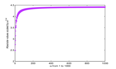
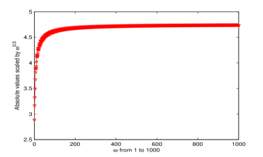
Figure 1: Absolute values of (3.15) scaled by $\omega^{0.4}$ with $\nu=0,\alpha=-0.6,\beta=-0.3$ (left), and $\omega^{0.5}$ with $\nu=0.3,\alpha=-0.5,\beta=-0.2$ (right), respectively, when $\omega$ runs from $1$ to $1000$.

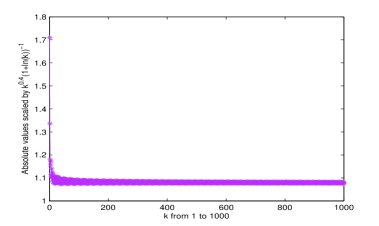
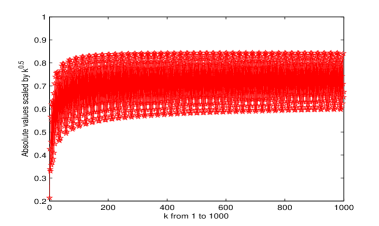
Figure 2: Absolute values of (3.16) scaled by $k^{0.4}\left(1+\ln(k)\right)^{-1}$ with $\nu=0,\alpha=-0.6,\beta=-0.3$ (left), and $k^{0.5}$ with $\nu=0.3,\alpha=-0.2,\beta=-0.4$ (right), respectively, when $k$ runs from $1$ to $1000$.

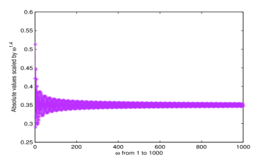
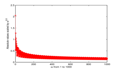
Figure 3: Absolute values of (3.17) scaled by $\omega^{1.4}$ with $\nu=0,\alpha=0.4,\beta=0.5$ (left), and $\omega^{0.5}$ with $\nu=0.3,\alpha=-0.2,\beta=-0.5$ (right), respectively, when $\omega$ runs from $1$ to $1000$.

Theorem 3.2

Suppose that $f(x)$ is a sufficiently smooth function on $[0,1]$, then for each $\alpha-|\nu|>-1,\beta>-1$ and fixed $N$, the error bound on $k$ and $\omega$ for the Clenshaw–Curtis–Filon–type method (2.3) for the integral (1.1) can be estimated by the following three formulas.

(i) For fixed $k$, when $\omega\rightarrow\infty$, there holds

$$I[f]-Q_{N,s}^{CCF}[f]=O\left(\frac{1}{\omega^{s+2+\tau_{1}}}\right).$$ (3.18)

where $\tau_{1}=\min\left\{\alpha,\beta\right\}$.

(ii) For fixed $\omega$, when $k\rightarrow\infty$, there holds

$$I[f]-Q_{N,s}^{CCF}[f]=\left\{\begin{array}[]{ll}O\left(\frac{1+\ln\left(k\right)}{k^{s+2+\alpha}}\right),&\hbox{$\nu=0,\alpha\leq\beta$},\\ O\left(\frac{1}{k^{s+2+\beta}}\right),&\hbox{$\nu=0,\alpha<\beta$},\\ O\left(\frac{1}{k^{s+2+\tau_{2}}}\right),&\hbox{$\nu\neq 0$},\end{array}\right.$$ (3.22)

where $\tau_{2}=\min\left\{\alpha-|\nu|,\beta\right\}$.

(iii) For a special case that $\omega=2k$, when $\omega\rightarrow\infty$, there holds

$$I[f]-Q_{N,s}^{CCF}[f]=O\left(\frac{1}{\omega^{s+2+\tau_{1}}}\right).$$ (3.23)

4 Numerical examples

In this section, we will present several examples to illustrate the efficiency and accuracy of the proposed method. Throughout the paper, all numerical computations were implemented on the R2012a version of the Matlab system. The experiments were performed on a computer with 3.20 GHz processor and 4 GB of RAM. In addition, the exact values of all the considered integrals $I[f]$ were computed in the Maple 17 using 32 decimal digits precision arithmetic.

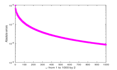
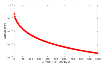
Figure 4: Absolute errors for the Clenshaw–Curtis–Filon–type method for the integral (4.1) with $s=0$ (left) and $s=1$ (right), when $N=4$, $k=50$, $\omega$ from $1$ to $1000$ by 2.

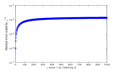
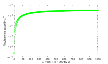
Figure 5: Absolute errors scaled by $\omega^{1.4}$ with $s=0$ (left) and $\omega^{2.4}$ with $s=1$ (right) for the Clenshaw–Curtis–Filon–type method for the integral (4.1) when $N=4$, $k=50$, $\omega$ from $1$ to $1000$ by 2.

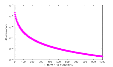
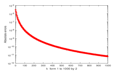
Figure 6: Absolute errors for the Clenshaw–Curtis–Filon–type method for the integral (4.2) with $s=1$ (left) and $s=2$ (right), when $N=6$, $\omega=50$, $k$ from $1$ to $1000$ by 2.

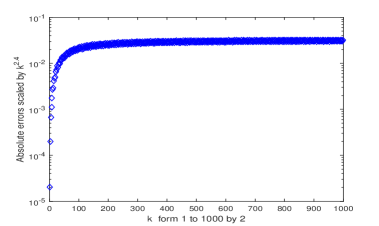
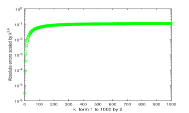
Figure 7: Absolute errors scaled by $k^{2.4}$ with $s=1$ (left) and $k^{3.4}$ with $s=2$ (right) for the Clenshaw–Curtis–Filon–type method for the integral (4.2) when $N=6$, $\omega=50$, $k$ from $1$ to $1000$ by 2.

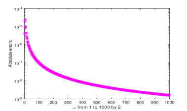
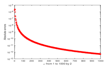
Figure 8: Absolute errors for the Clenshaw–Curtis–Filon–type method for the integral (4.3) with $s=0$ (left) and $s=1$ (right), when $N=4$, $\omega$ from $1$ to $1000$ by 2.

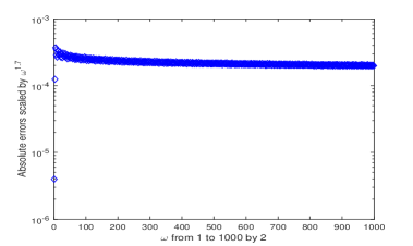
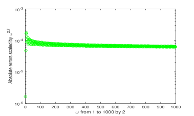
Figure 9: Absolute errors scaled by $\omega^{1.7}$ with $s=0$ (left) and $\omega^{2.7}$ with $s=1$ (right) for the Clenshaw–Curtis–Filon–type method for the integral (4.3) when $N=4$, $\omega$ from $1$ to $1000$ by 2.

Table 1: Relative errors for the integral (4.1) by the Clenshaw–Curtis–Filon–type method with $k=10$, $N=2,4,6$ and $s=0,1,2$.

$s$	$N$	$\omega=10$	$\omega=20$	$\omega=50$
$0$	$2$	$1.78\times 10^{-4}$	$1.35\times 10^{-4}$	$7.60\times 10^{-5}$
	$4$	$1.35\times 10^{-6}$	$8.93\times 10^{-7}$	$5.22\times 10^{-7}$
	$6$	$3.34\times 10^{-9}$	$1.97\times 10^{-9}$	$1.20\times 10^{-9}$
$1$	$2$	$3.94\times 10^{-7}$	$1.96\times 10^{-7}$	$5.32\times 10^{-8}$
	$4$	$1.04\times 10^{-9}$	$6.75\times 10^{-10}$	$1.71\times 10^{-10}$
	$6$	$1.72\times 10^{-12}$	$9.28\times 10^{-13}$	$2.49\times 10^{-13}$
$2$	$2$	$6.56\times 10^{-10}$	$2.20\times 10^{-10}$	$4.47\times 10^{-11}$
	$4$	$1.48\times 10^{-12}$	$3.74\times 10^{-13}$	$7.76\times 10^{-14}$
	$6$	$1.89\times 10^{-15}$	$6.79\times 10^{-16}$	$1.26\times 10^{-16}$
Real Values		$0.841824877078759$	$0.708386698058846$	$0.517419675175559$
		$-1.172097304662626\,\mathrm{i}$	$-0.956797421788702\,\mathrm{i}$	$-0.711685588704216\,\mathrm{i}$

Table 2: Relative errors for the integral (4.2) by the Clenshaw–Curtis–Filon–type method with $\omega=10$, $N=8,16,24$ and $s=0,1,2$.

$s$	$N$	$k=80$	$k=160$	$k=320$
$0$	$8$	$4.36\times 10^{-4}$	$2.19\times 10^{-4}$	$1.11\times 10^{-4}$
	$16$	$1.51\times 10^{-6}$	$8.45\times 10^{-7}$	$4.13\times 10^{-7}$
	$24$	$3.11\times 10^{-9}$	$1.12\times 10^{-9}$	$3.53\times 10^{-10}$
$1$	$8$	$4.80\times 10^{-6}$	$8.59\times 10^{-7}$	$2.62\times 10^{-7}$
	$16$	$7.80\times 10^{-8}$	$1.48\times 10^{-8}$	$3.37\times 10^{-9}$
	$24$	$7.96\times 10^{-10}$	$1.28\times 10^{-10}$	$2.61\times 10^{-11}$
$2$	$8$	$7.96\times 10^{-7}$	$8.89\times 10^{-8}$	$1.19\times 10^{-8}$
	$16$	$8.10\times 10^{-9}$	$7.17\times 10^{-10}$	$7.77\times 10^{-11}$
	$24$	$2.95\times 10^{-11}$	$1.81\times 10^{-12}$	$1.37\times 10^{-13}$
Real Values		$0.030083151162300$	$0.023581342870858$	$0.017909179561849$
		$-0.042241981991079\,\mathrm{i}$	$-0.031875514971454\,\mathrm{i}$	$-0.024353985798652\,\mathrm{i}$

Table 3: Relative errors for the integral (4.3) by the Clenshaw–Curtis–Filon–type method with $N=3,6,9$ and $s=0,1,2$.

$s$	$N$	$\omega=25$	$\omega=50$	$\omega=100$
$0$	$3$	$2.26\times 10^{-5}$	$9.40\times 10^{-6}$	$4.04\times 10^{-6}$
	$6$	$1.33\times 10^{-6}$	$5.97\times 10^{-7}$	$2.75\times 10^{-7}$
	$9$	$2.59\times 10^{-9}$	$1.29\times 10^{-9}$	$6.98\times 10^{-10}$
$1$	$3$	$2.03\times 10^{-6}$	$4.66\times 10^{-7}$	$1.11\times 10^{-7}$
	$6$	$5.78\times 10^{-10}$	$1.60\times 10^{-10}$	$2.41\times 10^{-11}$
	$9$	$4.42\times 10^{-11}$	$1.32\times 10^{-11}$	$2.82\times 10^{-12}$
$2$	$3$	$1.25\times 10^{-8}$	$1.98\times 10^{-9}$	$2.74\times 10^{-10}$
	$6$	$1.86\times 10^{-10}$	$2.26\times 10^{-11}$	$2.37\times 10^{-12}$
	$9$	$2.11\times 10^{-13}$	$7.48\times 10^{-15}$	$2.98\times 10^{-15}$
Real Values		$0.030229145167903$	$0.017639904837672$	$0.010310330002264$
		$-0.034246416918332\,\mathrm{i}$	$-0.019163197919570\,\mathrm{i}$	$-0.010688289764988\,\mathrm{i}$

Example 4.1. Let us consider the computation of the integral

$$\int_{0}^{1}x^{\alpha}(1-x)^{\beta}\cos(x)\mathrm{e}^{\mathrm{i}2kx}H_{\nu}^{(1)}(\omega x)\,\mathrm{d}x$$ (4.1)

by the Clenshaw–Curtis–Filon–type method (2.3), where $\nu=0,\alpha=-0.6,\beta=-0.3$. The absolute errors and scaled absolute errors are displayed in Figs. 4–5, respectively. Also, the relative errors are displayed in Table 1.

Example 4.2. Let us consider the computation of the integral

$$\int_{0}^{1}x^{\alpha}(1-x)^{\beta}\frac{1}{1+16x^{2}}\mathrm{e}^{\mathrm{i}2kx}H_{\nu}^{(1)}(\omega x)\,\mathrm{d}x$$ (4.2)

by the Clenshaw–Curtis–Filon–type method (2.3), where $\nu=0.6,\alpha=0,\beta=-0.3$ (Figs. 6–7, Table 2).

Example 4.3. Finally, we consider the computation of the integral of a special form

$$\int_{0}^{1}x^{\alpha}(1-x)^{\beta}\frac{1}{1+(1+x)^{2}}\mathrm{e}^{\mathrm{i}\omega x}H_{\nu}^{(1)}(\omega x)\,\mathrm{d}x$$ (4.3)

by the Clenshaw–Curtis–Filon–type method (2.3), where $\nu=0.3$, and $\alpha=-0.2,\beta=-0.3$. Figs. 6–7 show error bound on $\omega$ for the Clenshaw–Curtis–Filon–type method for this case. Table 3 displays the relative errors for the proposed method with $N=3,6,9$ and $s=0,1,2$.

Form Figs. 5, 7, 9, we can see that the error bounds given in Theorem 3.2 for the Clenshaw–Curtis–Filon–type method are attainable. Figs. 4, 6, 8 and Tables 1–3 show that the presented method is very efficient for the approximation of the integral (1.1). Moreover, for the well-behaved function $f(x)$, the integral (1.1) can be efficiently approximated by Clenshaw–Curtis–Filon–type method with a small number of interpolation points. In addition, the improvement of the accuracy for the integral (1.1) can be obtained by using interpolation with derivatives of higher order at two endpoints, or adding the number of the interpolation points.

5 Concluding remarks

In this paper, we consider a Clenshaw–Curtis–Filon–type method for the computation of the integral (1.1) with $(N+1)$ Clenshaw–Curtis points, which can be efficiently implemented in $O(N\log N)$ operations. Moreover, we present a universal method for the derivation of the recurrence relation for the modified moments, which can be applied to the modified moments with other type kernels. Based on this recurrence relation, the modified moments can be efficiently computed by using the special functions or the existing method with small number of points. Finally, an error bound on $k$ and $\omega$ and several numerical experiments are given to show the accuracy and efficiency for the proposed method.

References

- [1] M. Abramowitz and I.A. Stegun, Handbook of Mathematical Functions, National Bureau of Standards, Washington, D.C., 1964.
- [2] S. Arden, S.N. Chandler–Wilde and S. Langdon, A collocation method for high-frequency scattering by convex polygons, J. Comput. Appl. Math. 204 (2007) 334–343.
- [3] G. Arkfen, Mathematical Methods for Physicists, third ed., Academic Press, Orlando, Fl, 1985.
- [4] G. Bao, W. Sun, A fast algorithm for the electromagnetic scattering form a large cavity, SIAM J. Sci. Comput. 27 (2005) 553–574.
- [5] H. Bateman, A. Erdélyi, Higher Transcendental Functions, Vol. I, McGraw–Hill, New York, 1953.
- [6] N. Bleistein and R. Handelsman, A generalization of the method of steepest escent, IMA J. Numer. Anal. 10 (1972) 211–230.
- [7] R. Chen, Numerical approximations to integrals with a highly oscillatory Bessel kernel, Appl. Numer. Math. 62 (2012) 636–648.
- [8] R. Chen, On the evaluation of Bessel transformations with the oscillators via asymptotic series of Whittaker functions, J. Comput. Appl. Math. 250 (2013) 107–121.
- [9] R. Chen, C. An, On evaluation of Bessel transforms with oscillatory and algebraic singular integrands, J. Comput. Appl. Math. 264 (2014) 71–81.
- [10] R. Chen, Numerical approximations for highly oscillatory Bessel transforms and applications, J. Math. Anal. Appl. 421 (2015) 1635–1650.
- [11] P. J. Davis and D. B. Duncan, Stability and convergence of collocation schemes for retarded potential integral equations, SIAM J. Sci. Comput. 42 (2004) 1167–1188.
- [12] V. Domínguez, I. G. Graham, V. P. Smyshlyaev, Stability and error estimates for Filon–Clenshaw–Curtis rules for highly–oscillatory integrals, IMA J. Numer. Anal. 31 (2011) 1253–1280.
- [13] V. Domínguez, I. G. Graham, T. Kim, Filon–Clenshaw–Curtis rules for highly-oscillatory integrals with algebraic singularities and stationary points, SIAM J. Numer. Anal. 51 (2013) 1542–1566.
- [14] A. Erdélyi, Asymptotic representations of Fourier integrals and the method of stationary phase, J. Soc. Ind. Appl. Math. 3 (1955) 17–27.
- [15] G. A. Evans and J. R. Webster, A high order progressive method for the evaluation of irregular oscillatory integrals, Appl. Numer. Math. 23 (1997) 205–218.
- [16] G. A. Evans and K. C. Chung, Some theoretical aspects of generalised quadrature methods, J. Complex. 19 (2003) 272–285.
- [17] L. N. G. Filon, On a quadrature formula for trigonometric integrals, Proc. Royal. Soc. Edinburgh. 49 (1928), 38–47.
- [18] G. He, S. Xiang and E. Zhu, Efficient computation of highly oscillatory integrals with weak singularity by Gausstype method, Int. J. Comput. Math. (2014). doi: 10.1080/00207160.2014.987761.
- [19] http://functions.wolfram.com/HypergeometricFunctions/Hypergeometric0F1/26/02/13/0001/.
- [20] http://functions.wolfram.com/HypergeometricFunctions/Hypergeometric0F1/26/02/15/0001/.
- [21] D. Huybrechs and S. Vandewalle, On the evaluation of highly oscillatory integrals by analytic continuation, SIAM J. Numer. Anal. 44 (2006), 1026–11048.
- [22] D. Huybrechs and S. Vandewalle, A sparse discretisation for integral equation formulations of high frequency scattering problems, SIAM J. Sci. Comput. 29 (2007) 2305–2328.
- [23] A. Iserles and S. P. Nørsett, Efficient quadrature of highly oscillatory integrals using derivatives, Proc. Royal Soc. A. 461 (2005), 1383–1399.
- [24] H. Kang and S. Xiang, Efficient quadrature of highly oscillatory integrals with algebraic singularities, J. Comput. Appl. Math. 237 (2013), 576–588.
- [25] H. Kang, S. Xiang and G. He, Computation of integrals with oscillatory and singular integrands using Chebyshev expansions, J. Comput. Appl. Math. 242 (2013), 141–156.
- [26] H. Kang and X. Shao, Fast computation of singular oscillatory Fourier transforms, Abstr. Appl. Anal. (2014) 1–8, art. no. 984834.
- [27] H. Kang and C. Ling, Computation of integrals with oscillatory singular factors of algebraic and logarithmic type, J. Comput. Appl. Math. 285 (2015), 72–85.
- [28] D. Levin, Fast integration of rapidly oscillatory functions, J. Comput. Appl. Math. 67 (1996) 95–101.
- [29] D. Levin, Analysis of a collocation method for integrating rapidly oscillatory functions, J. Comput. Appl. Math. 78 (1997) 131–138.
- [30] D. W. Lozier, Numerical solution of linear difference equations, Report NBSIR 80-1976, National Bureau of Standerds, Washington, D.C., 1980.
- [31] Y. L. Luke, The Special Functions and Their Approximations, Vol. I., Academic Press, London, 1969.
- [32] J. C. Mason and D. C. Handscomb, Chebyshev Polynomials, Chapman and Hall/CRC, New York, 2003.
-
[33]
http://functions.wolfram.com/HypergeometricFunctions/MeijerG/21/02/07/00
01/. - [34] J. Oliver, The numerical solution of linear recurrence relations, Numer. Math. 11 (1968) 349–360.
- [35] S. Olver, Numerical approximation of vector-valued highly oscillatory integrals, BIT Numer. Math. 47 (2007) 637–655.
-
[36]
B. Oreshkin, http://www.mathworks.com/matlabcentral/fileexchange/31490-meijerg/content/
MeijerG/MeijerG.m. - [37] R. Piessens, M. Branders, On the computation of Fourier transforms of singular functions, J. Comput. Appl. Math. 43 (1992) 159–169.
- [38] I. H. Sloan and W. E. Smith, Product-integration with the Clenshaw–Curtis and related points, Numer. Math. 30 (1978) 415–428.
- [39] I. H. Sloan and W. E. Smith, Product integration with the Clenshaw–Curtis points: implementation and error estimates, Numer. Math. 34 (1980) 387–401.
- [40] S. Xiang, Efficient Filon-type methods for , Numer. Math. 105 (2007), 633–658.
- [41] S. Xiang and H. Wang, Fast integration of highly oscillatory integrals with exotic oscillators, Math. Comput. 79 (2010) 829–844.
- [42] S. Xiang, Y. Cho, H. Wang and H. Brunner, Clenshaw–Curtis–Filon–type methods for highly oscillatory Bessel transforms and applications, IMA J. Numer. Anal. 31 (2011) 1281–1314.
- [43] Z. Xu, S. Xiang, Numerical evaluation of a class of highly oscillatory integrals involving Airy functions, Appl. Math. Comput. 246 (2014) 54–63.
- [44] Z. Xu, G.V. Milovanović and S. Xiang, Efficient computation of highly oscillatory integrals with Hankel kernel, Appl. Math. Comput. 261 (2015) 312–322.
- [45] Z. Xu, S. Xiang, On the evaluation of highly oscillatory finite Hankel transform using special functions, Numer. Algor. (2015) doi: 10.1007/s11075-015-0033-3.