Computer model calibration with large non-stationary spatial outputs: application to the calibration of a climate model

Abstract

Bayesian calibration of computer models tunes unknown input parameters by comparing outputs with observations. For model outputs that are distributed over space, this becomes computationally expensive because of the output size. To overcome this challenge, we employ a basis representation of the model outputs and observations: we match these decompositions to carry out the calibration efficiently. In the second step, we incorporate the non-stationary behaviour, in terms of spatial variations of both variance and correlations, in the calibration. We insert two integrated nested Laplace approximation-stochastic partial differential equation parameters into the calibration. A synthetic example and a climate model illustration highlight the benefits of our approach.

Keywords: Gaussian process; integrated nested Laplace approximations-stochastic partial differential equation; Matérn fields; uncertainty quantification

1 Introduction

Complex computer models are widely used in various fields of science and technology to mimic complex physical systems. Computer model calibration involves comparing the simulations of a complex computer model with the physical observations of the process being simulated. Increasingly, computer model outputs are in the form of spatial fields, particularly in environmental sciences. This poses a particular challenge to the calibration method.

The class of models that we consider in this paper are computer models with parametric inputs of reasonable dimension (say below 20), and outputs distributed over two dimensions over the plane or the sphere. This is unlike the Kennedy and O’Hagan formulation (Kennedy and O’Hagan, 2001), which is usually applied to scalar outputs. Our motivations come from climate modelling. Climate scientists compare model outputs at a certain relevant altitude distributed over the sphere, typically over a grid (along latitude and longitude), with a spatial data set of observations at the same altitude.

In this paper, we develop our Bayesian calibration technique based on the framework from Kennedy and O’Hagan (2001): we approximate the expensive computer model by a Gaussian process (GP). This formulation has proven to be effective in a wide range of applications. However, the GP calibration is computationally expensive for large model output spaces (cubic complexity in the number of output points used to fit the GP due to the Cholesky decomposition). Therefore several attempts to tackle this issue in the context of times series of outputs or spatial outputs have been made either by using truncated basis representations of model outputs in order to reduce dimension (Bayarri et al., 2007; Higdon et al., 2008; Chang et al., 2014; Holden et al., 2015), or by using a separable covariance function over space and tuning parameters to build a theoretical emulator for multivariate outputs (Rougier, 2008; Bhat et al., 2010). We provide here a solution that makes use of an adequate representation of the spatial outputs using Gaussian fields.

Gaussian fields (GFs) play an important role in spatial statistics. The traditional approach is to specify a GF through its covariance function. Another approach is to use the class of Gaussian Markov random fields (GMRFs), which are discretely indexed GFs. The Markov property yields a sparse precision matrix, so that efficient numerical algorithms can be employed. Lindgren et al. (2011) show that the GMRF representation can be constructed explicitly by using a certain form of stochastic partial differential equation (SPDE) which has a GF with Matérn covariance as its solution. The representation employs piecewise linear basis functions, and Gaussian weights with Markov dependences determined by the finite element method over a triangulation of the domain. This technique can deal with large spatial data sets and naturally account for nonstationarity. Our paper combines the strengths of the calibration formulation with a truncated basis, and the SPDE defined scale and precision parameterization to deal with large scale spatial outputs, and still provides a compromise with computational feasibility in order to employ a fully Bayesian approach.

1.1 Challenge in Bayesian calibration

Among existing approaches of using the basis representation of model outputs, dimension reduction is carried out mostly by data-driven basis functions, i.e. principal components (PCs), also known as empirical orthogonal functions (EOFs), see Higdon et al. (2008). Data-driven basis functions offer a computationally efficient approach to adapt the outputs. For the propose of computer model calibration of spatial outputs, this approach ignores the nature of the spatial dependence of the outputs, treating spatial data as a multivariate vector.

Since the dimension of the input space for known input parameters is two (the location in space), we could employ the usual calibration framework (Kennedy and O’Hagan, 2001). However, this framework can only deal with few thousands of output points at these input locations. But climate models produce outputs over large regular grid cells, e.g. our climate model uses a grid of $n=96\times 144=13824$ cells, and this is at a rather coarse choice of resolution. We calibrate four input parameters with $r=100$ runs, thus the number of computer runs $r$, multiplied by the output size $n$ creates a data matrix that is too large to fit a GP, an impossible task for a fully Bayesian calibration (cubic complexity in the total number of output points to fit the GP). Hence our approach aims to reduce the large amount of model outputs with a smaller basis representation that makes use of the spatial dependency to extract key pieces of information, instead of using all the output cells. Our approach involves transforming a large scalar output over space into a much smaller set of scalars by using a spherical harmonics representation and the SPDE technique.

1.2 Atmospheric chemistry model output

We consider that an atmospheric chemistry model discretizes Earth’s surface into a three-dimensional grid of cells over time, which can be characterized by horizontal (latitude and longitude), vertical (altitude or pressure level) and temporal resolutions. The output in each cell is parameterized by complex mathematical equations that describe the chemistry species in it and the physical circulation through it. The four dimensional interactions of climate dynamics are currently beyond our scope for the calibration. Our paper only focuses on the horizontal variations. Our practical interest is to tune, and quantify uncertainty in, climate experiments. The Whole Atmosphere Community Climate Model (WACCM) is a general circulation model of the middle and upper atmosphere. WACCM is an extension of the National Center for Atmospheric Research (NCAR) Community Earth System Model (CESM). Many parameterizations of physical processes have to be set to run WACCM, resulting in potential concerns about error growth (Liu et al., 2009).

To describe the general framework, let $\eta(\mathbf{s}_{i},\bm{\theta}_{j}),i=1,\ldots,n;j=1,\ldots,r$ be the $r$-runs model outputs measured at $n$ locations. Here we refer to $m=n\times r$ as the total number of outputs in the simulations. We choose a design made of combinations of input values, and we impose distributional prior assumptions on the inputs. The aim of calibration is to estimate the best input setting $\bm{\theta}^{\ast}$ to match outputs to observations, and investigate the discrepancy between observations and optimized outputs. Note that in terms of the calibration framework from Kennedy and O’Hagan (2001), our experiment does not have ‘known variable parameters’, output cells are prescribed as a resolution in the climate model, thus the spatial variations in different model runs are completely differentiated by calibration inputs $\bm{\theta}$.

For each single run, WACCM simulates output over a grid of $n=96\times 144=13824$ cells. We explore the zonal wind outputs over the sphere, varying according to four gravity wave (GW) input parameters with $r=100$ runs, in order to calibrate the GW parameters. The number of computer runs $r$, multiplied by the output size $n$ is too large to fit a GP to the computer model, and thus challenges the fully Bayesian calibration to be performed.

1.3 The propagation of gravity waves

In climate modeling, the GWs parametrization aims to reduce zonal mean wind biases. Small modification of parameterized GWs can have large impacts by improving the propagation pathways of the Rossby waves (Alexander and Sato, 2015). GWs also play a dominant role in driving the quasi-biennial oscillation (QBO), which is a dynamic process of zonal mean zonal winds from eastward to westward in the tropical stratosphere. GWs, also called small-scale atmospheric waves, generate a wide range of short horizontal wavelengths from mesoscale to thousands of kilometers (Ern et al., 2014), and an even wider range of the processes impacted by GWs (turbulence scales to planetary scales) (Liu et al., 2014). It is thus a challenge to numerically simulate all small waves and their cumulated effects that contribute to QBO pattern based on global observations (Alexander et al., 2010; Geller et al., 2013; Yu et al., 2017).

1.4 Outline of this paper

We propose to use a fixed spatial basis, as Bayarri et al. (2007) did by employing a wavelets basis to describe for functional model outputs. Our approach is also related to recent multi-resolution methods on spatial data (Nychka et al., 2002, 2015; Ilyas et al., 2017). With a fixed basis, we can easily compare model outputs to observations over space. In addition, the use of a fixed basis facilitates the quantification of the non-stationarity across space in the SPDE model.

In Section 2 we present our approach in detail. We employ a truncated basis representation, such as a B–splines decomposition or spherical harmonics transforms, to capture the output features spatially. We then explore how parameters in an SPDE model can explicitly quantify the nonstationarity of the the spatial field (Bolin and Lindgren, 2011; Blangiardo and Cameletti, 2015; Zammit-Mangion et al., 2015; Liu et al., 2016): we extend our approach by including spatially-varying scale and precision parameters in an SPDE model into our calibration framework. We then apply these techniques to a synthetic example in Section 3 and our real climate experiment in Section 4. Finally in Section 5, we discuss potential improvements to our approach.

2 Methods

To address the challenges of the uncertainty quantification at both global and local scales, and maintain computational feasibility for the Bayesian calibration, we pursue a sophisticated effort that approximate the spatial variations effectively and efficiently. In section 2.1, we adopt a reduced rank spatial basis representation to capture the large scale spatial variability. In the next step in Section 2.2, we review the spatial modeling technique through the SPDE approach, and highlight its strength in capturing local spatial structures. We then combine these two approaches into the calibration framework in Section 2.3, and provide a guidance for the implementation in Section 2.4.

2.1 Basis representation for the model output

In this section, we decompose spatial outputs and observations onto a basis of real valued basis functions, such as B–splines or spherical harmonics. We parsimoniously represent these surfaces, and construct a methodology for the calibration that makes use of the coefficients in these representations. We follow the Bayesian calibration setting of Kennedy and O’Hagan (2001). Let $\bm{\theta}$ be the calibration parameters. The output $\eta(\cdot)$ is computed at inputs $(\mathbf{s},\bm{\theta})$ in an $m$-point experimental design, where $m=n\times r$ means $r$ computer runs measured at $n$ locations. The output $\eta(\mathbf{s},\bm{\theta})$ is an approximation of the reality $y^{R}(\mathbf{s})$. The discrepancy between the simulator and the reality at the spatial locations is denoted $\delta(\mathbf{s})$. The observations $y^{F}(\mathbf{s})$ of reality are collected at a number of locations $\mathbf{s}$ in an $n$-point spatial design (here a simple grid), and are subject to a normal observation error $\epsilon(\mathbf{s})$ with a constant variance across locations. The measurement locations for observations and outputs can be different, since the methodology accommodates such variation. The main equation is:

$$y^{F}(\mathbf{s})=y^{R}(\mathbf{s})+\epsilon(\mathbf{s})=\eta(\mathbf{s},\bm{\theta}^{\ast})+\delta(\mathbf{s})+\epsilon(\mathbf{s}).$$ (1)

This formulation includes both parameter uncertainty and model discrepancy, however, it is hard to distinguish the uncertainty in the calibration parameters from discrepancy in real applications due to lack of identifiability (Brynjarsdóttir and O’Hagan, 2014). Note that output cells are prescribed as a model resolution, the uncertainties in $\eta$ are completely determined by $\bm{\theta}$. We use a set of spatial basis functions $\{\psi_{z}\}$, where $z$ is an integer that represents the index number within the ordered basis, to decompose each run of model output over space. Precisely, for the $N_{\eta}$-th level of expansion and for each run $j$:

$$\eta(\mathbf{s},\bm{\theta}_{j})=\sum_{z=1}^{N_{\eta}}c^{M}_{z}(\bm{\theta}_{j})\psi_{z}(\mathbf{s})\qquad j=1,\ldots,r.$$

We assume that the approximation error in this representation is ignorable (i.e., we expect the more bases, the lower approximation error). The coefficients $\{c^{M}_{z}\}$ represent the surface features at different levels of expansion. Similar to Nychka et al. (2015), we conjecture that different spatial basis functions will be valid for this representation, such as the Wendland family (Wendland, 2004) used in Nychka et al. (2015) or popular spline-based approaches (Wood, 2003; Williamson et al., 2012; Chakraborty et al., 2013; Bowman and Woods, 2016; Chang et al., 2017). The observations can be written as (with an associated approximation error ignored):

$$y^{F}(\mathbf{s})=\sum_{z=1}^{N_{y}}c^{F}_{z}\psi_{z}(\mathbf{s}).$$

The physical space of both model outputs and observations are transformed into a functional space spanned by the fixed basis. Since the aim is to calibrate the spatial outputs, we also assume that the reality $y^{R}(\mathbf{s})$, the discrepancy function $\delta(\mathbf{s})$, and the measurement errors $\epsilon(\mathbf{s})$, can be represented by similar basis representations, albeit with more levels of variation than model outputs:

$$y^{R}(\mathbf{s})=\sum_{z=1}^{N_{y}}c^{R}_{z}\psi_{z}(\mathbf{s}),\qquad\delta(\mathbf{s})=\sum_{z=1}^{N_{y}}c^{\delta}_{z}\psi_{z}(\mathbf{s}),\qquad\epsilon(\mathbf{s})=\sum_{z=1}^{N_{y}}c^{\epsilon}_{z}\psi_{z}(\mathbf{s}).$$

Indeed, the computer model does not include all possible physical processes that affect the measurements. Hence, the spatial outputs from the computer simulation should be relatively smoother than the observations. Therefore we assume a larger number of basis functions ($N_{y}$) in the observations (automatically as well in the discrepancy and error functions) than for model outputs ($N_{\eta}$, $N_{\eta}\leq N_{y}$). In the formulation of the calibration algorithm, we introduce coefficients $\{c^{M}_{z}|N_{\eta}<z\leq N_{y}\}$, all set to be $\mathbf{0}$. Indeed, we are then able to use the same number of basis functions $N_{y}$ to decompose $y^{F}$ and $\eta$. Then matching the coefficients in (1) yields:

$$c_{z}^{F}=c_{z}^{R}+c^{\epsilon}_{z}=c_{z}^{M}(\bm{\theta}^{\ast})+c_{z}^{\delta}+c^{\epsilon}_{z},\qquad z=1,\ldots,N_{y}.$$ (2)

Hence, only the relatively smooth variations of the computer model match the variations in observations. At this point we only seek to capture the large scale variability derived from calibration parameters, local structures will be accounted for in Section 2.2. The weights for the measurement errors, $c^{\epsilon}_{z}$, are assumed to follow $N(0,1/\lambda_{\epsilon})$.

2.1.1 GP for the transformed coefficients

The GP assumption is imposed on each coefficient $c^{M}_{z}(\bm{\theta}),z=1,\ldots,N_{y}$, of mean 0 and with a covariance function

$$\text{Cov}(c^{M}_{z}(\bm{\theta}),c^{M}_{z^{\prime}}(\bm{\theta}^{\prime}))=\frac{1}{\lambda_{\eta}}I_{zz^{\prime}}\prod_{k=1}^{q}\rho_{\eta k}^{2^{\gamma_{\eta k}}|\theta_{k}-\theta^{\prime}_{k}|^{\gamma_{\eta k}}},$$ (3)

where $I_{zz^{\prime}}$ is the Kronecker’s delta ($I_{zz^{\prime}}=1$ if $z=z^{\prime}$ and 0 otherwise), $q$ is the dimension of $\bm{\theta}$, $\lambda_{\eta}$ controls the marginal precision of $\eta(\cdot,\cdot)$ and $\bm{\rho}_{\eta}$ controls the strength of the dependence in each of the pairs of $\bm{\theta}$. To simplify the complexity and due to computer model response to input tunes is nearly smooth and continuity, it is generally reasonable to assume $\bm{\gamma}_{\eta}=2$ (Sacks et al., 1989; Higdon et al., 2004; Linkletter et al., 2006). Note that the coefficients $\{c^{M}_{z}\}$ have to be scaled to the unit hypercube, otherwise this covariance model is not appropriate. This reparameterization of the square exponential covariance leads to a smooth and infinitely differentiable representation for the model output (Stein, 1999). In addition, coefficients associated to same basis $\psi_{z}$ form a block in the covariance structure, and we assume that the correlation between different indices $z$ is 0. Hence the $rN_{y}$-vector $\mathbf{c}^{M}$ has a multivariate normal prior with mean 0 and a covariance matrix with $r\times r$’s $N_{y}$ blocks in the diagonal, and the off-diagonal blocks are zero matrices.

The strong assumption of independence of the coefficients, through different blocks in the covariance, may not be fully justifiable in all real applications. Indeed, it is possible that certain physical properties propagate across multiple scales (but even in that case, it may not constitute a large proportion of the variation). However, this assumption leads to a great computational advantage in terms of forming a block diagonal covariance model in the GP model. Traditionally a GP fitting involves a complexity of $O(m^{3})=O(n^{3}r^{3})$ and a storage cost of $O(m^{2})=O(n^{2}r^{2})$. In our approach the complexity and cost of our model are $O(N_{y}^{3}r^{3})$ and $O(N_{y}^{2}r^{2})$, where $N_{y}<<n$. The block diagonal assumption further reduces the complexity and cost to $O(N_{y}r^{3})$ and $O(N_{y}r^{2})$. In simulation study we discuss how this assumption is a compromise between fidelity and complexity.

The decomposed discrepancy term $c_{z}^{\delta}$ quantifies the inadequacy between the simulator and reality in the functional domain. We assume that each $c^{\delta}_{z}$ follows a normal distribution of mean 0 and with a covariance function:

$$\text{Cov}(c^{\delta}_{z},c^{\delta}_{z^{\prime}})=\frac{1}{\lambda_{\delta}}I_{zz^{\prime}}.$$ (4)

There is no conceptual difference in the model bias between our setting and another setting that relies on a projection onto a basis (e.g. the PC approach), but there are differences in the ability to concretely and adequately pin down the biases. Indeed, our approach allows the bias to represent complex ranges of variations (due to its expression in a basis and the addition of nonstationarity in the sequel of this paper). Note that among existing studies identifying climate model biases, most of the biases display a systematic tendency (either underestimation or overestimation) across certain regions (Jun et al., 2008; Lamarque et al., 2013; Wang et al., 2014; Williamson et al., 2015) and thus a nonstationarity feature is desirable.

All the unknown parameters in the algorithm require specified prior distributions which represent uncertainty about the values of these parameters. The following choices are made for the priors: (a) To represent our vague knowledge about calibration parameters, we specify a uniform prior distribution over each of the calibration parameter interval; (b) To model the correlation parameters $\rho_{\eta_{k}},k=1,\ldots,q$, a Beta(1, 0.1) distribution is used, which conservatively places most of its prior mass on values of $\bm{\rho}_{\eta}$ near 1 (indicating an insignificant effect); (c) Gamma prior distributions are used for each of the precision parameters $\lambda_{\eta}$, $\lambda_{\delta}$ and $\lambda_{\epsilon}$. Specifically, we use priors $\lambda_{\eta}\sim$ GAM(5, 5) (with expectation 1 due to standardization of the responses), $\lambda_{\delta}\sim$ GAM(1, 0.01) (with expectation around 10% of SD of the standardized responses) and $\lambda_{\epsilon}\sim$ GAM(1, 0.003) (with expectation around 5% of SD of the standardized responses).

2.1.2 The posterior distributions

In this stage, all the $r$-run model outputs and observations, measured over an $n$-grid cells, are reduced to transformed coefficients. Denote the joint $(r+1)N_{y}$ data vector $\mathbf{D}=(c^{F},c^{M})$. The sampling likelihood for the full data is then

$$L(\mathbf{D}|\bm{\theta},\lambda_{\eta},\bm{\rho}_{\eta},\lambda_{\delta},\Sigma_{\epsilon})\propto|\Sigma_{\mathbf{D}}|^{-1/2}\exp\left\{-\frac{1}{2}(\mathbf{D}^{T}\Sigma_{\mathbf{D}}^{-1}\mathbf{D})\right\},$$ (5)

where

$$\Sigma_{\mathbf{D}}=\Sigma_{\eta}+\begin{pmatrix}\Sigma_{\epsilon}+\Sigma_{\delta}&0\\ 0&0\\ \end{pmatrix},$$

in which $\Sigma_{\epsilon}$ is the $N_{y}\times N_{y}$ observation covariance matrix, $\Sigma_{\eta}$ is obtained for each pair of $(r+1)N_{y}$ simulation inputs through (3) corresponding to $\mathbf{D}$, and $\Sigma_{\delta}$ is an $N_{y}\times N_{y}$ matrix obtained for each pair of $N_{y}$ input through the instances of (4) that correspond to the coefficients $c^{F}$. Let $\pi(\bm{\theta})$ be the joint prior distribution for the (unknown) calibration vector $\bm{\theta}$. The resulting posterior density has the form

$$\pi(\bm{\theta},\lambda_{\eta},\bm{\rho}_{\eta},\lambda_{\delta}|\mathbf{D})\propto L(\mathbf{D}|\bm{\theta},\lambda_{\eta},\bm{\rho}_{\eta},\lambda_{\delta},\Sigma_{\epsilon})\times\pi(\bm{\theta})\times\pi(\lambda_{\eta})\times\pi(\bm{\rho}_{\eta})\times\pi(\lambda_{\delta}),$$ (6)

which can be explored via a Markov chain Monte Carlo (MCMC) technique, for which we employ a Metropolis–Hastings algorithm. The calibrated vector is then denoted by $\bm{\theta}^{\ast}=\text{argmax}_{\theta}\pi(\bm{\theta},\lambda_{\eta},\bm{\rho}_{\eta},\lambda_{\delta}|\mathbf{D})$. We implement a Metropolis–Hastings algorithm to produce the realization of the posterior. Metropolis updates are used for the correlation and the calibration parameters with a uniform proposal distribution centered at the current value of the parameter. The precision parameters are sampled using Hastings updates with a uniform proposal distribution centered at the current value of the parameter (Higdon et al., 2008). This eventually yields draws from the posterior distribution by repeatedly accepting and rejecting a choice of move in the parameter space.

The specification of the covariance structures for the truncated basis representation is a mathematical challenge: finding explicit expressions for the covariance is hard (Jun and Stein, 2008). There is an alternative way to efficiently model complex spatial covariance structures with the added bonus of a suitable depiction of the nonstationarity structure into our calibration algorithm: the SPDE approach. We introduce it in the next section.

2.2 Spatial modeling through the SPDE approach

Traditional models in spatial statistics build an approximation of the entire underlying random field. They are usually specified through the covariance function of the latent field. In order to assess uncertainties in the spatial interpolation over the whole spatial domain, we cannot build models only for the discretely located observations or model outputs, we need to build an approximation of the entire underlying stochastic process defined on the spatial field. We consider statistical models for which the unknown functions are assumed to be realizations of a Gaussian random spatial process. The conventional fitting approach spatially interpolates values as linear combinations of the original observed locations, and this constitutes the spatial kriging predictor.

Due to the fixed underlying covariance structure, this approach requires more sophisticated treatments to take into consideration nonstationarity (Stein, 2005; Jun and Stein, 2008; Yue and Speckman, 2010; Kleiber and Nychka, 2012; Gramacy and Apley, 2015). A different computational approach was introduced by Lindgren et al. (2011), in which random fields are expressed as a weak solution to an SPDE, with explicit links between the parameters of the SPDE model and the Matérn covariance function. In this section we review some of the main concepts in spatial modeling through the SPDE approach.

It may seem contradictory to make use of the SPDE approach since it seemingly only captures local structures, and climate model outputs display smooth variations. However, the SPDE approach, especially the nonstationarity version, is able to translate these smooth variations of the model outputs (and of observations) into a statistical description of the variations across space that efficiently characterizes the spatial behaviour (through the scale and precision parameters). Spatially distributed observations will still display more erratic behaviour than model outputs, but the SPDE approach will allow the calibration to be steered only by the parameters associated with the smoothest components.

2.2.1 Matérn covariance and the link to SPDE

The Matérn function is a flexible covariance structure and widely used in the spatial statistics (Stein, 2005; Jun and Stein, 2007, 2008; Gneiting et al., 2010; Genton and Kleiber, 2015). The choice of covariance is not that important indeed for calibration parameters (Kennedy and O’Hagan, 2001), but for the outputs (across location inputs), the choice of covariance is essential, as we show. The shape parameter $\nu>0$, the scale parameter $\kappa>0$, and the marginal precision $\tau^{2}>0$, parameterize it:

$$\text{Cov}(\mathbf{h})=\frac{2^{1-\nu}}{(4\pi)^{d/2}\Gamma(\nu+d/2)\kappa^{2\nu}\tau^{2}}(\kappa\|\mathbf{h}\|)^{\nu}K_{\nu}(\kappa\|\mathbf{h}\|),\mathbf{h}\in\mathbb{R}^{d},$$

where $\mathbf{h}$ denotes the difference between any two locations $s$ and $s^{\prime}$: $\mathbf{h}=s-s^{\prime}$, and $K_{\nu}$ is the modified Bessel function of the second kind of order $\nu$.

We denote by $Y(\mathbf{s})$ the observations (or the spatially distributed model outputs) for a latent spatial field $X(\mathbf{s})$, with a Matérn covariance structure. We assume a zero mean Gaussian noise, $\mathcal{W}(\mathbf{s})$, with a constant variance $\sigma^{2}_{s}$: $Y(\mathbf{s})=X(\mathbf{s})+\mathcal{W}(\mathbf{s})$. Thus, according to Whittle (1963), the latent field $X(\mathbf{s})$ is the solution of a stationary SPDE:

$$(\kappa^{2}-\Delta)^{\alpha/2}\tau X(\mathbf{s})=\mathcal{W}(\mathbf{s}),$$ (7)

where $\Delta$ is the Laplace operator. We explain in the next paragraph how the analysis of this SPDE can be carried out by the finite element method. The regularity (or smoothness) parameter $\nu$ essentially determines the order of differentiability of the fields. The link between the Matérn field and the SPDE is given by $\alpha=\nu+d/2$, which makes explicit the relationship between dimension and regularity for fixed $\alpha$. On more general manifolds than $\mathbb{R}^{d}$, such as the sphere (Chang et al., 2015a), the direct Matérn representation is not easy to implement (for example, Matérn covariance with great circle distance is only valid at $\nu\in(0,0.5]$ (Gneiting, 2013)), but the SPDE formulation provides a natural generalization, and the $\nu$-parameter will keep its meaning as the quantitative measure of regularity. Instead of defining Matérn fields by the covariance function, Lindgren et al. (2011) used the solution of the SPDE as a definition, and it is much easier and flexible to do so. This definition also facilitates nonstationary extensions by allowing the SPDE parameters $\kappa$ and $\tau$ in Eq. (7) to vary with space, hence denoted $\kappa(\cdot)$ and $\tau(\cdot)$ respectively.

2.2.2 SPDE model construction

We estimate the SPDE parameters and supply uncertainty information about the spatial fields by using the integrated nested Laplace approximations (INLA) framework, available as an R package (http://www.r-inla.org/) (Lindgren and Rue, 2015; Rue et al., 2017). The models implemented in the INLA–SPDE framework are built on a basis representation (triangulation over the spatial domain): $X(\mathbf{s})=\sum_{i=1}^{M}\varphi_{i}(\mathbf{s})w_{i}$, where $\{w_{i}\}$ are the stochastic weights chosen so that the distribution of the functions $X(\mathbf{s})$ approximates the distribution of solutions to the SPDE on the space, and $\varphi_{i}(\mathbf{s})$ are piecewise linear basis with compact support (i.e. finite elements) in order to obtain a Markov structure, and to preserve it when conditioning on local observed locations. The Markov property yields a sparse precision matrix, so that efficient numerical algorithms can be employed for large spatial data. The projection of the SPDE onto the basis representation is chosen by a finite element method. The finite element method represents a general class of techniques for the approximate solution to partial differential equations. The piecewise linear basis functions defined by a triangulation of the spatial domain allow us to explicitly evaluate the precision matrix of the latent field. As a result, $X(\mathbf{s})$ follows a normal distribution with mean 0, and the precision matrix can be explicitly expressed as a combination of the piecewice linear basis functions weighted by $\kappa$ and $\tau$ (which means $\kappa$ and $\tau$ have a joint influence on the marginal variances of the latent field). Then $X(\mathbf{s})$ can be generated continuously as approximative solutions to the SPDE.

For the WACCM output domain, the triangulation is simply built upon regularly gridded cells. Note that the triangulation can be made adaptive to the irregularly distributed spatial data (Cameletti et al., 2013). The default value in INLA is $\alpha=2$, but $0\leq\alpha<2$ are also available, though yet to be completely tested (Lindgren and Rue, 2015). So, with a 2-dimensional manifold (e.g. $\mathbb{R}^{2}$ and $\mathbb{S}^{2}$), the smoothness parameter $\nu$ must be fixed at 1 due to the relationship $\alpha=\nu+d/2$. The strength of this SPDE technique enables us to quantify the level of nonstationarity by employing spatial basis representations for both $\kappa$ and $\tau$ (i.e. these quantities are constants in a stationary field). With a focus on the calibration, let $\kappa^{M}(\mathbf{s},\bm{\theta})$ and $\tau^{M}(\mathbf{s},\bm{\theta})$ be the scale and precision parameters in an SPDE model used to approximate the model outputs. To obtain basic identifiability, $\kappa^{M}(\mathbf{s},\bm{\theta})$ and $\tau^{M}(\mathbf{s},\bm{\theta})$ are taken to be positive, and their logarithm can be decomposed as:

$$\log\kappa^{M}(\mathbf{s},\bm{\theta}_{j})=\sum_{z=1}^{N_{\kappa}}\kappa^{M}_{z}(\bm{\theta}_{j})\psi_{z}(\mathbf{s}),\quad\text{and}\quad\log\tau^{M}(\mathbf{s},\bm{\theta}_{j})=\sum_{z=1}^{N_{\tau}}\tau^{M}_{z}(\bm{\theta}_{j})\psi_{z}(\mathbf{s}),\quad j=1,\ldots,r.$$

Each basis function is evaluated at output cells and observed locations. The coefficients $\{\kappa^{M}_{z}\}$ and $\{\tau^{M}_{z}\}$ represent local variances and correlation ranges (Bolin and Lindgren, 2011; Lindgren et al., 2011; Fuglstad et al., 2015). For the sake of simplicity, we call these coefficients ‘SPDE parameters’ in the calibration. We introduce in next section how to incorporate the SPDE parameters into calibration in order to enhance the prediction accuracy.

2.3 Combining SPDE modeling and calibration

A reduced rank approach was often used to ease the computational issue in large spatial data sets (Banerjee et al., 2008; Cressie and Johannesson, 2008; Furrer and Sain, 2009; Katzfuss and Cressie, 2011). In order to reduce and summarize a spatial field properly, both global and local scale dependences need to be well captured and represented. To do so, a two steps approximation was developed by combining the reduced rank representation and sparse matrix techniques, to account for global and local structures, respectively (Stein, 2007; Sang and Huang, 2012). We follow the same idea of using a reduced rank representation to capture global scale variability (described in Section 2.1), while instead of tapering the covariance matrix into sparse, we use the INLA-SPDE technique to represent small scale variability. In this section we describe the details of our extension by including the SPDE defined scale and precision parameters into the Bayesian calibration.

As $\{\kappa^{M}_{z}(\bm{\theta})\}$ and $\{\tau^{M}_{z}(\bm{\theta})\}$ can quantify the nonstationarity and derivative information in the spatial process, we now include these two types of coefficients into our technique (combined with $\{c^{M}_{z}(\bm{\theta})\}$ in the previous section, and vectorized all coefficients as a scalar). Then our approach represents the observations and model input–output relationship as follows:

$$y^{F}(s_{1}),\ldots,y^{F}(s_{n}) \xrightarrow{\text{transform}}c^{F}_{1},\ldots,c^{F}_{N_{y}},\kappa^{F}_{1},\ldots,\kappa^{F}_{N_{\kappa}},\tau^{F}_{1},\ldots,\tau^{F}_{N_{\tau}}$$

$$\eta(s_{1},\theta_{1}),\ldots,\eta(s_{n},\theta_{1}) \xrightarrow{\text{transform}}c_{1}^{M}(\theta_{1}),\ldots,c^{M}_{N_{y}}(\theta_{1}),\kappa^{M}_{1}(\theta_{1}),\ldots,\kappa^{M}_{N_{\kappa}}(\theta_{1}),\tau^{M}_{1}(\theta_{1}),\ldots,\tau^{M}_{N_{\tau}}(\theta_{1})$$

$$\vdots$$

$$\eta(s_{1},\theta_{r}),\ldots,\eta(s_{n},\theta_{r}) \xrightarrow{\text{transform}}c_{1}^{M}(\theta_{r}),\ldots,c^{M}_{N_{y}}(\theta_{r}),\kappa^{M}_{1}(\theta_{r}),\ldots,\kappa^{M}_{N_{\kappa}}(\theta_{r}),\tau^{M}_{1}(\theta_{r}),\ldots,\tau^{M}_{N_{\tau}}(\theta_{r})$$

where $N_{y}+N_{\kappa}+N_{\tau}<<n$. The aim is to combine the SPDE parameters as nonstationary information for the implementation of the calibration algorithm, and to model all coefficients jointly with the GP assumption. We also assume that the three types of coefficients are independent. To describe the formulation of the design matrix, let $\{z_{1},z_{2},z_{3}|z_{1}=1,\ldots,N_{y};z_{2}=1,\ldots,N_{\kappa};z_{3}=1,\ldots,N_{\tau}\}$ be the indices used to represent each triplet of coefficients, respectively. The calibration formulation is hence:

$$\begin{pmatrix}c^{F}_{z_{1}}\\ \kappa^{F}_{z_{2}}\\ \tau^{F}_{z_{3}}\end{pmatrix}=\begin{pmatrix}c^{M}_{z_{1}}(\bm{\theta})\\ \kappa^{M}_{z_{2}}(\bm{\theta})\\ \tau^{M}_{z_{3}}(\bm{\theta})\end{pmatrix}+\begin{pmatrix}c^{\delta}_{z_{1}}\\ \kappa^{\delta}_{z_{2}}\\ \tau^{\delta}_{z_{3}}\end{pmatrix}+\begin{pmatrix}c^{\epsilon}_{z_{1}}\\ \kappa^{\epsilon}_{z_{2}}\\ \tau^{\epsilon}_{z_{3}}\end{pmatrix}.$$

Thus there are $(N_{y}+N_{\kappa}+N_{\tau})$-blocks of coefficients corresponding to each combination of $\bm{\theta}_{j},j=1\ldots,r$ in the covariance matrix. The GP assumption is imposed on each coefficient $(c^{M}_{z_{1},j},\kappa^{M}_{z_{2},j},\tau^{M}_{z_{3},j})^{T}$ with mean 0 and covariance function

$$\text{Cov}((c^{M}_{z_{1}}(\bm{\theta}),\kappa^{M}_{z_{2}}(\bm{\theta}),\tau^{M}_{z_{3}}(\bm{\theta}))^{T},(c^{M}_{z^{\prime}_{1}}(\bm{\theta}^{\prime}),\kappa^{M}_{z^{\prime}_{2}}(\bm{\theta}^{\prime}),\tau^{M}_{z^{\prime}_{3}}(\bm{\theta}^{\prime}))^{T})=\frac{1}{\lambda_{\eta}}\prod_{i=1}^{3}I_{z_{i}z^{\prime}_{i}}\prod_{k=1}^{q}\rho_{\eta k}^{4(\theta_{k}-\theta^{\prime}_{k})^{2}},$$

where $I_{z_{i}z^{\prime}_{i}}=1$ if $z_{i}=z^{\prime}_{i}$ and 0 otherwise. In other words, these 3 types of coefficients $\{{c}^{M}_{z_{1}},\kappa^{M}_{z_{2}},\tau^{M}_{z_{3}}\}$ have a joint multivariate normal prior distribution with mean 0, and a covariance structure forming a block diagonal matrix:

$$\begin{pmatrix}c^{M}_{z_{1}}\\ \kappa^{M}_{z_{2}}\\ \tau^{M}_{z_{3}}\end{pmatrix}\sim N\left(\mathbf{0},\begin{pmatrix}\text{Cov}(c^{M}_{z_{1}}(\bm{\theta}),c^{M}_{z^{\prime}_{1}}(\bm{\theta}^{\prime}))&0&0\\ 0&\text{Cov}(\kappa^{M}_{z_{2}}(\bm{\theta}),\kappa^{M}_{z^{\prime}_{2}}(\bm{\theta}^{\prime}))&0\\ 0&0&\text{Cov}(\tau^{M}_{z_{3}}(\bm{\theta}),\tau^{M}_{z^{\prime}_{3}}(\bm{\theta}^{\prime}))\\ \end{pmatrix}\right).$$

The elements in each block are also block diagonal matrices. The model discrepancy term in the functional space follows a GP assumption defined in Equation (4). All the prior assumptions discussed in the previous section remain unchanged. Thus the sampling likelihood in (5) and the posterior distribution in (6) still hold in this case. Overall, we decompose the model outputs into a basis via the coefficients $\{c^{M}\}$, and estimate the SPDE parameters $\{\kappa^{M},\tau^{M}\}$ in the latent field through a regression onto these basis functions. We are essentially fitting a GP model with $\{c^{M}\}$ for the regression mean structure and $\{\kappa^{M},\tau^{M}\}$ for the parameters of Matérn covariance function.

2.4 Guidance for the number of basis functions

In real applications, we often do not know whether the calibrated values work until actually performing a validation. It can be computationally challenging to find the optimized orders for the combination of $N_{y}$, $N_{\kappa}$ and $N_{\tau}$. Similar to most truncated basis representations, we choose the number of basis functions post hoc. We provide the following model selection guidelines: (1) The basis representation for the mean structure of model outputs play a dominant role in the algorithm. Typically we cannot expect to calibrate a global process only through a local structure. Therefore $N_{y}$ usually needs to be greater than $N_{\kappa}+N_{\tau}$; (2) Calibration with only one of the coefficients $\kappa$ or $\tau$ cannot improve the analysis. The reason is the fact that $\kappa$ and $\tau$ represent a spatial process jointly being tacitly assumed. Recall that the Matérn function is controlled by the smoothness parameter $\nu$, the scale parameter $\kappa$, and the precision parameter $\tau$. The parameter $\nu$ is fixed by $\alpha=\nu+d/2$ in connection with the SPDE, thus the approximated spatial process depends upon $\kappa$ and $\tau$ jointly. Both $\kappa$ and $\tau$ need to be included to reflect the full variation in the spatial field.

In this paper we use spherical harmonics (SHs) as our primary investigation. The SHs represent the wave features at different scales on the sphere (Bolin and Lindgren, 2011; Jun and Stein, 2008). For the purpose of calibration, it seems unnecessary in general to approximate the spatial processes with very high order expansions of SHs to fit each run of model output best. The main requirement is to extract sufficient and meaningful information about the calibration parameters from the variations in the SH coefficients that could be attributed to variations in the inputs. To ensure that this requirement is met, a simple validation is to increase the basis number and re-calibrate the model. In case the results have no statistically significant impacts, then the number is large enough. Muir and Tkalčić (2015) utilized the corrected Akaike information criterion (AIC) to choose an optimal maximum order of expansion for an irregular data on the sphere in a hierarchical Bayesian setting. The results show the 3rd to 5th order of expansion in SHs are generally a turning point from fast to slow reduction in AIC in terms of balancing explanatory power with simplicity (although not the smallest AIC). In all these approaches, the choice of the number of basis vectors is currently post hoc. We reckon that the 3rd or 4th order of SH transform for capturing large scale variability, along with a lower order of SPDE nonstationary information to account for local structure, as a good start in practical application.

3 Simulation Study: Nonstationary field

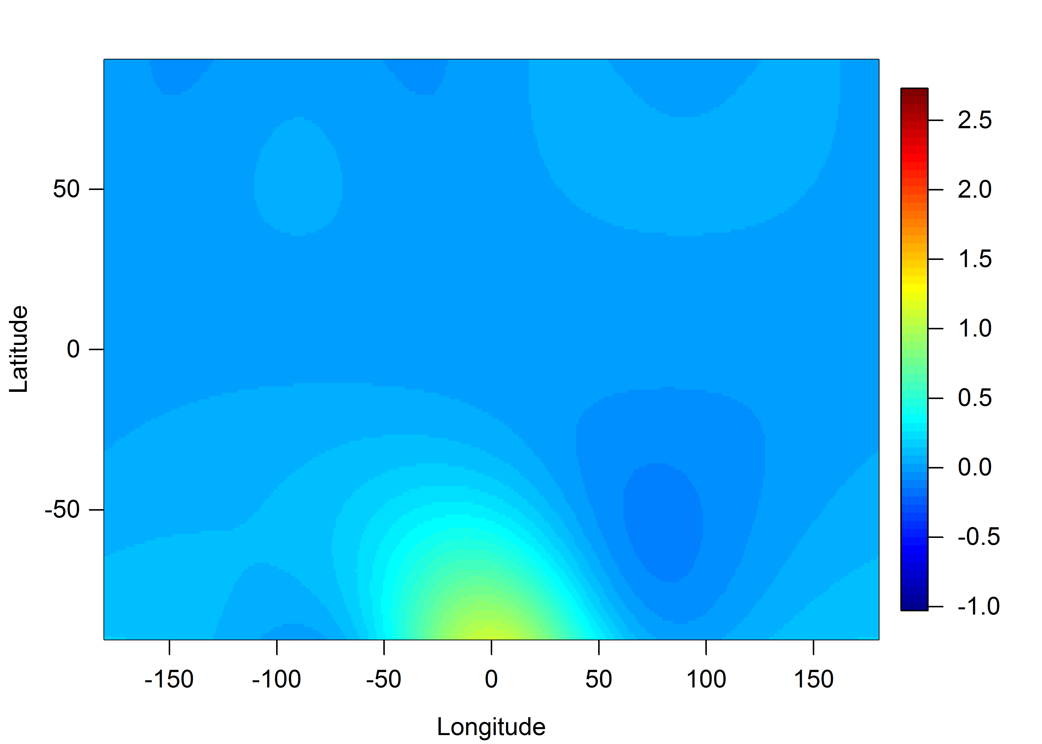
(a) Combined surface

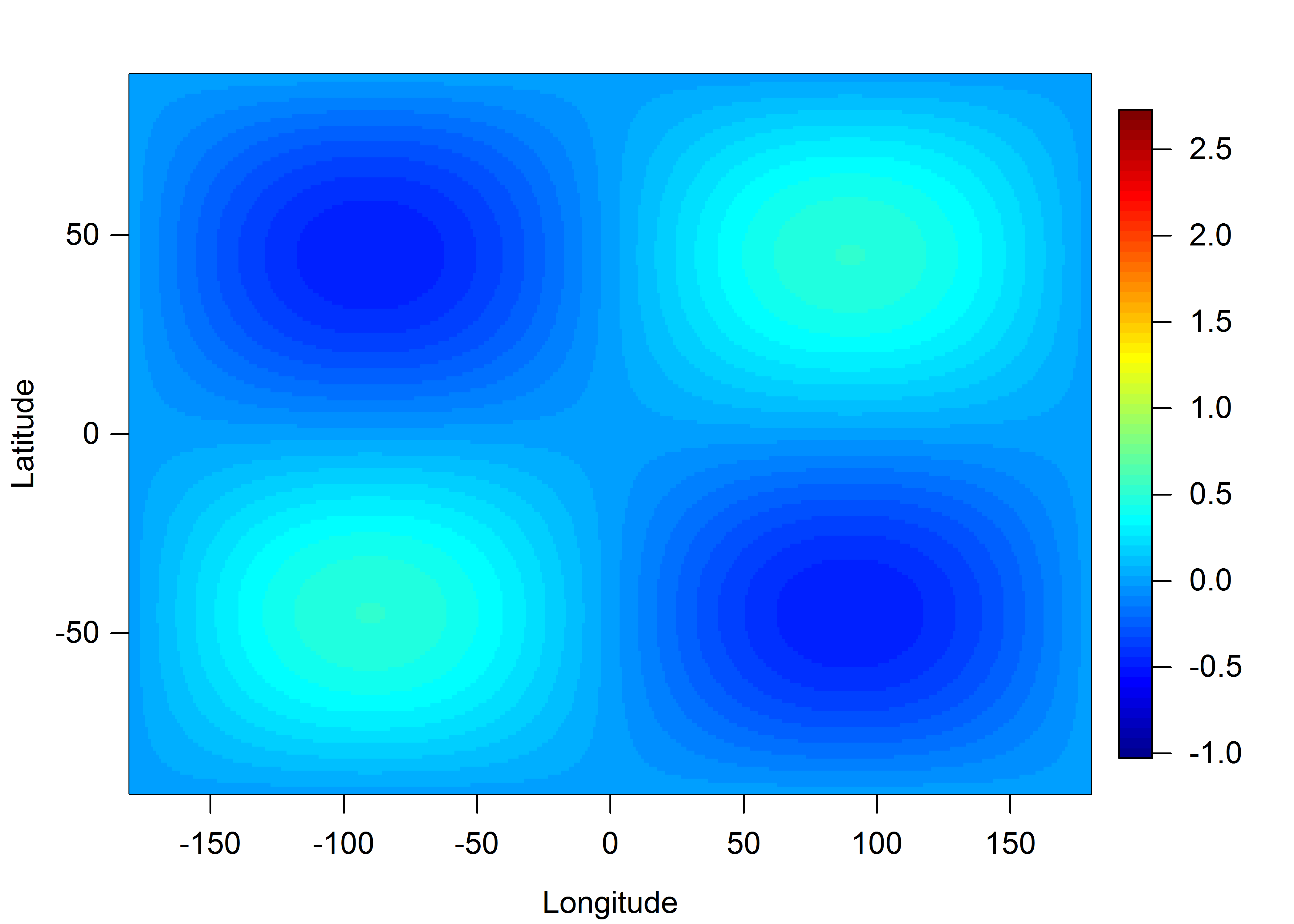
(b) $s_{2}s_{3}$

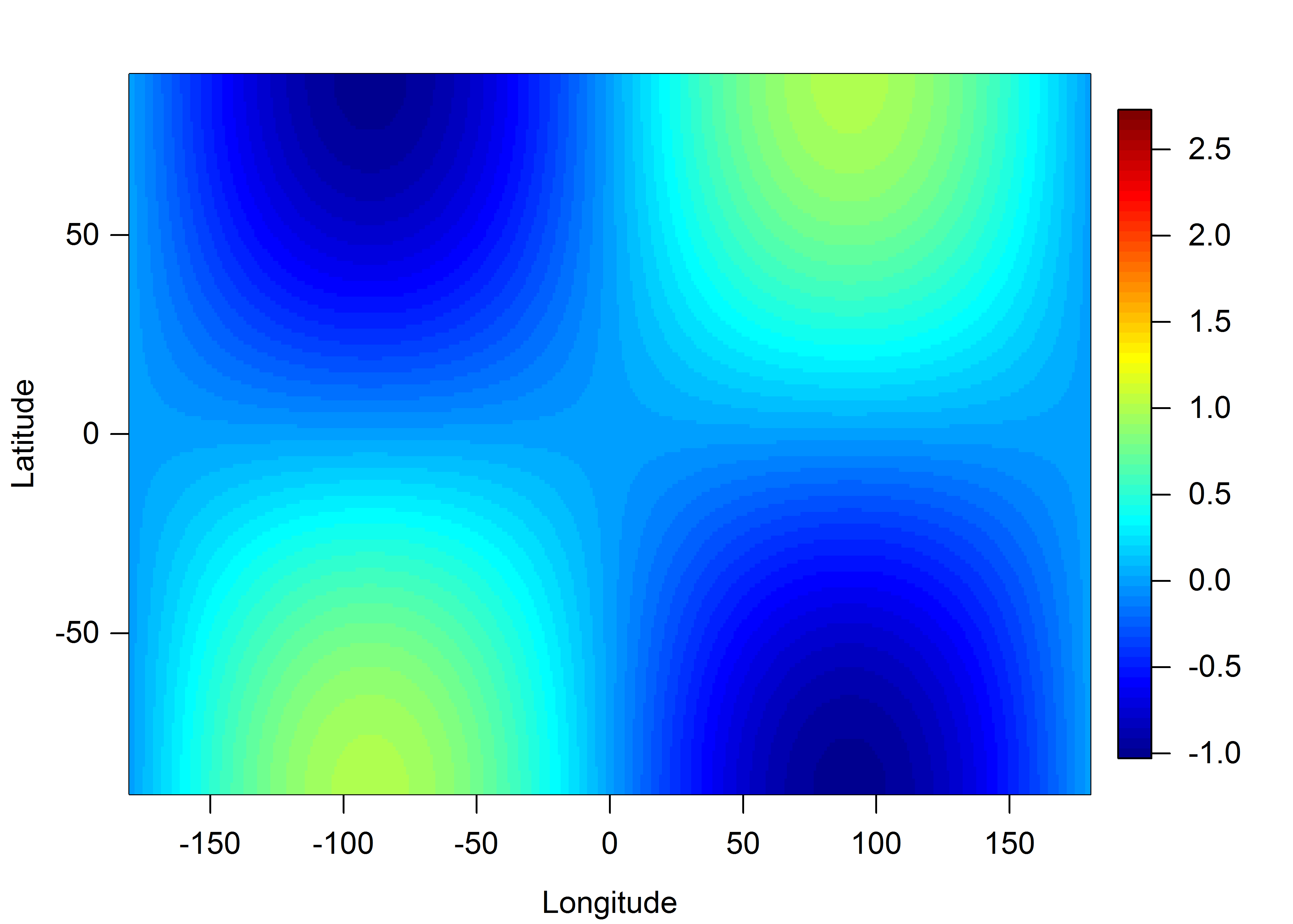
(c) $s_{2}$

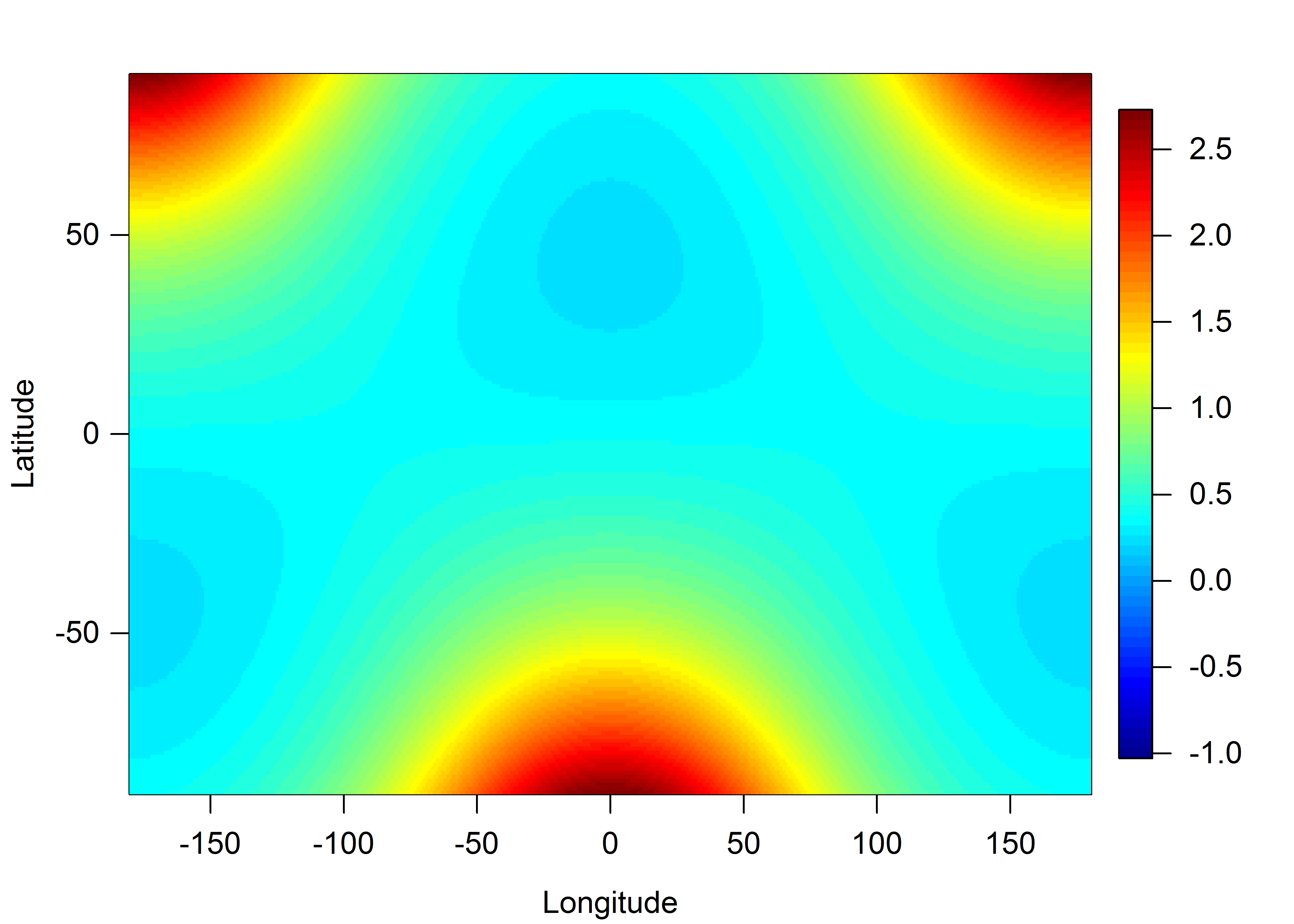
(d) $\exp(-s_{3}-s_{1})$

Figure 1: Combined synthetic observed surface and each spatial component in function (8).

In order to illustrate the methodology, this synthetic example simulates a nonstationary field on the sphere, with an anisotropic property (the spatial correlation depends on latitude), to demonstrate how including the parameters in the SPDE can enhance the GP calibration in such situations. We illustrate how the parameters in an SPDE technique can be incorporated into our calibration algorithm to model nonstationarity over a spherical domain. With $n=10\times 10$ regularly spaced locations in latitude ($L$) and longitude ($l$), and $r=50$ computer runs according to a maximin latin hypercube design (LHD) for the calibration inputs, the function with three calibration parameters ($q=3$) is set to

$$f(\tilde{\mathbf{s}},\bm{\theta})=(0.5s_{1}^{2}+\theta_{1}s_{2}s_{3})\times\left\{\begin{array}[]{l l}\theta_{2}s_{2}&\quad\text{if $L>\pi/2$}\\ \theta_{3}\exp(-s_{3}-s_{1})&\quad\text{if $L\leq\pi/2$}\end{array}\right.,(\theta_{1},\theta_{2},\theta_{3})\in[0,1]^{3},$$ (8)

where the true values for $(\theta_{1},\theta_{2},\theta_{3})$ are set to $(0.5,0.2,0.8)$, and $(s_{1},s_{2},s_{3})=(\cos(l)\sin(L),\sin(l)\sin(L),\cos(L))$ are spherical coordinates. We create a nonstationary spatial field by introducing different structures in the Northern and Southern hemispheres, where $\theta_{1}$ is a global calibration parameter, and $(\theta_{2},\theta_{3})$ are local variates. Note that in this example the local structures are designed to be larger than global structure: $\exp(-s_{3}-s_{1})$ has stronger variation than $s_{2}$, and both of them have a larger variation than $s_{2}s_{3}$ (see the magnitude of variation in each component from Fig. 1).

First, we perform the spherical harmonics transform (SHT) onto observations $y^{F}$ and each computer run $\eta_{j},j=1,\ldots,50$, and then carry out the calibration on the coefficients. In total, we estimate 13 models with different numbers of expansion order. The results of using the 4th to 7th orders of the SHT are shown in the first part of Table 1 (Strategies A-D). We can see that the global calibration parameter $\theta_{1}$ is estimated well. However, even though the convergence of an MCMC chain can be established for $\theta_{2}$ and $\theta_{3}$, the posterior means are underestimated. According to the root-mean-square error (RMSE) between assumed and predicted observations, which can be written as

$$\text{RMSE}=\sqrt{\frac{\sum_{i=1}^{n}\left(f(s_{i},\bm{\theta}^{\ast})-f(s_{i},\bm{\theta}^{post})\right)^{2}}{n}},$$

an increase in the expansion order cannot improve the results. This underestimation can be viewed as a deficiency to capture local variations through a global mean structure: the variation created by these two parameters will be obscured and distorted by the variation from $\theta_{1}$.

Table 1: Posterior mean and SD for $(\theta_{1},\theta_{2},\theta_{3})$ in function (8), RMSE and number of coefficients (right column) under different orders of SHT for $\{\eta,\kappa,\tau\}$ per model run (RMSE was multiplied by $10^{3}$ to illustrate the magnitude).

Strategy	$\eta$	$\kappa$	$\tau$	$\theta_{1}$(=0.5)	$\theta_{2}$(=0.2)	$\theta_{3}$(=0.8)	RMSE	$N_{y}+N_{\kappa}+N_{\tau}$
A	4	-	-	0.505(0.050)	0.188(0.048)	0.762(0.038)	92	15
B	5	-	-	0.498(0.053)	0.179(0.062)	0.746(0.050)	132	21
C	6	-	-	0.477(0.062)	0.166(0.079)	0.705(0.069)	237	28
D	7	-	-	0.488(0.112)	0.198(0.127)	0.695(0.119)	257	36
E	-	1	1	0.579(0.158)	0.148(0.068)	0.620(0.200)	431	6
F	-	2	2	0.560(0.097)	0.189(0.078)	0.740(0.089)	145	12
G	-	3	3	0.785(0.078)	0.442(0.155)	0.858(0.054)	433	20
H	4	1	1	0.452(0.097)	0.071(0.049)	0.495(0.037)	755	21
I	5	1	1	0.495(0.044)	0.133(0.049)	0.498(0.032)	737	27
J	6	1	1	0.356(0.050)	0.135(0.052)	0.686(0.119)	322	34
K	4	2	2	0.553(0.068)	0.225(0.108)	0.771(0.109)	80	27
L	5	2	2	0.529(0.068)	0.179(0.107)	0.794(0.098)	28	33
M	6	2	2	0.537(0.066)	0.171(0.110)	0.789(0.083)	39	40

In order to understand the role of the SPDE parameters in the calibration, we then perform a calibration using only the coefficients $\{\kappa^{M},\tau^{M}\}$. Under the same priors and algorithm, the posterior mean and SD of the first three orders of the expansion for $\kappa^{M}$ and $\tau^{M}$ are shown in the second part of Table 1 (Strategies E - G). Even though the calibration does not fully succeed (and should not without matching original outputs to observations but only SPDE information), the result in the 2nd order expansion for $\kappa^{M}$ and $\tau^{M}$ seems informative as the posterior modes are close to the true values. The first two orders of the expansion surface for $\kappa^{F}$ and $\tau^{F}$ for the observations are shown in Fig. 2. It is difficult to directly interpret the features of $\kappa(s)$ and $\tau(s)$. However, from Fig. 2(c)-(d) we can see that a strong northeast-southwest flow in $\kappa^{F}(s)$ matches the pattern in Fig. 1 (b)-(c), and a highly anti-correlation between $\tau^{F}(s)$ (inverse precision) and $y^{F}$ surface.

For the next step, we infer $\{c^{M},\kappa^{M},\tau^{M}\}$ jointly with the GP model. We combined the coefficients in Strategies A-C (coefficients for the mean structure) and Strategies E-F (coefficients for the SPDE parameters). The results are presented in the third part of Table 1. We can see that with the SPDE information included, we achieve an improvement in the calibration by combining local structure with a global process. For example, Strategies C and K have a similar number of coefficients, but the combination with SPDE increases the estimated accuracy in $\theta_{2}$ and $\theta_{3}$. The similar case of Strategies D and L also supports the use of SPDE information. Strategy L uses a smaller number of coefficients, while achieving an improvement in terms of increased accuracy in $\theta_{3}$ and reduced RMSE. Nevertheless, only in the case of the 2nd order expansion do the SPDE parameters help; the 1st order expansion cannot achieve a good result in this example. This demonstrates that the nonstationarity is rather complex. From these findings we thus acknowledge that the SPDE technique enables us to identify the local feature from the global spatial process in the calibration. Therefore we highlight that when we cannot make an improvement in estimation accuracy by increasing the basis number into the mean structure, the SPDE technique can serve as a valuable alternative.

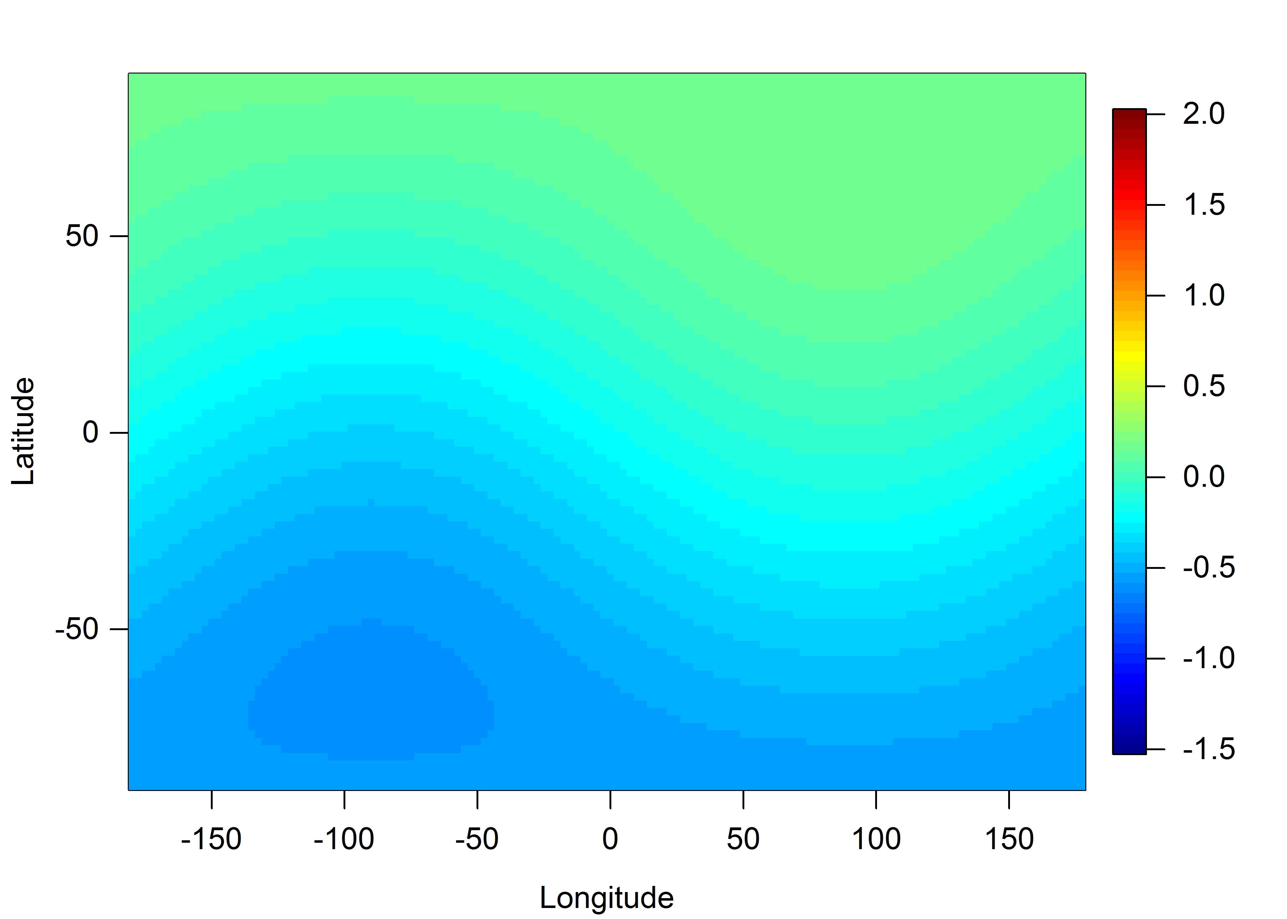
(a) 1st order $\kappa^{F}$

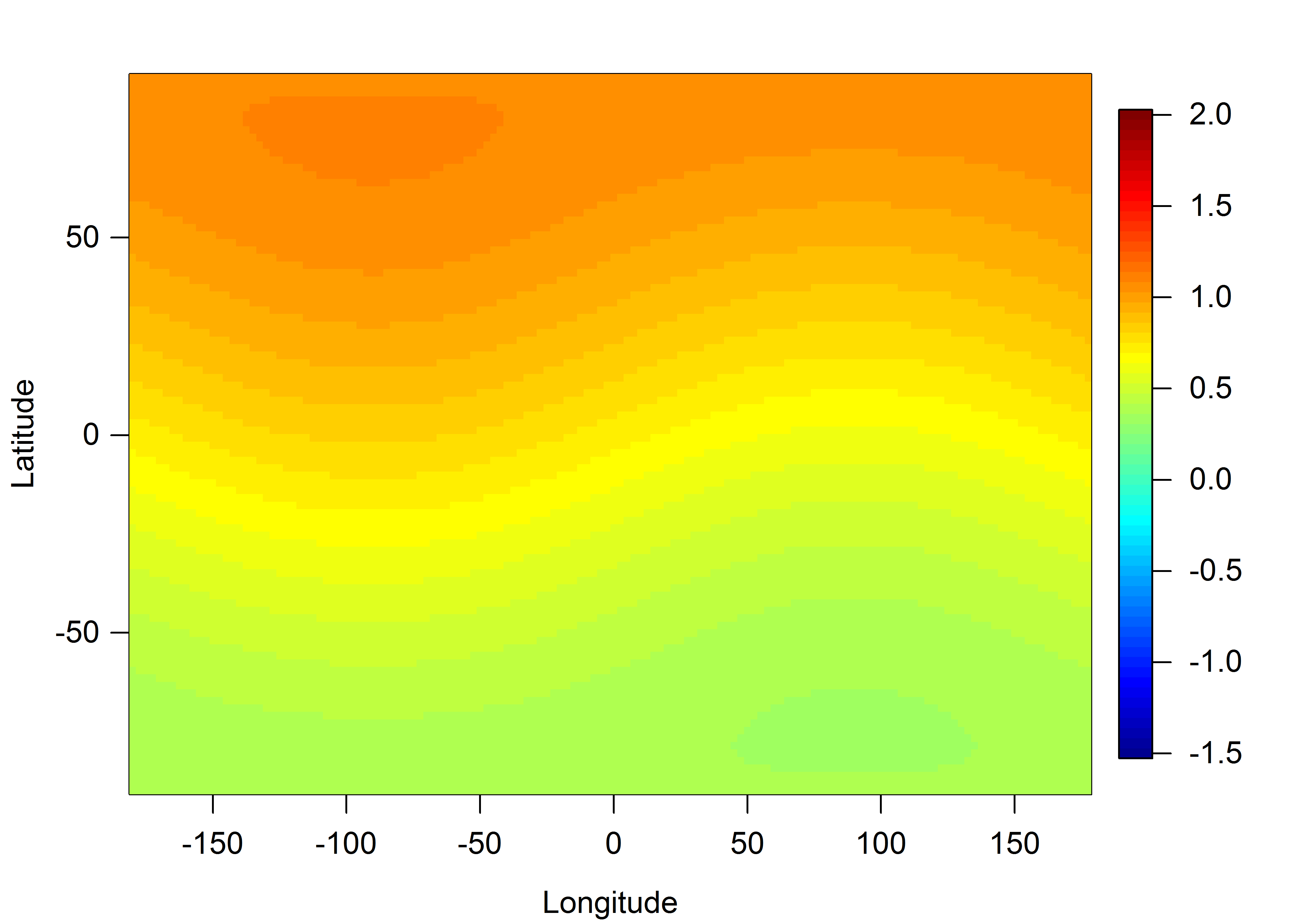
(b) 1st order $\tau^{F}$

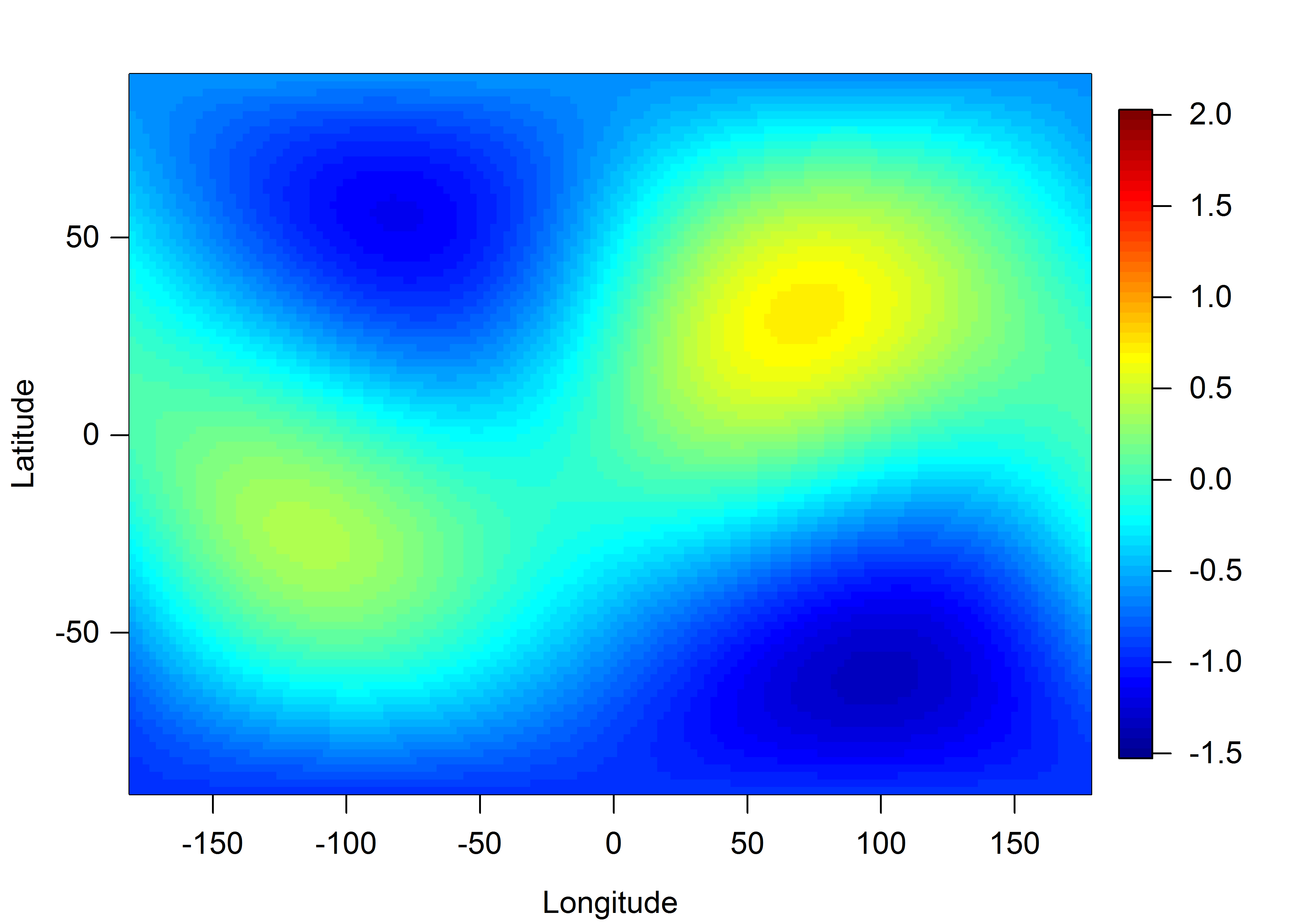
(c) 2nd order $\kappa^{F}$

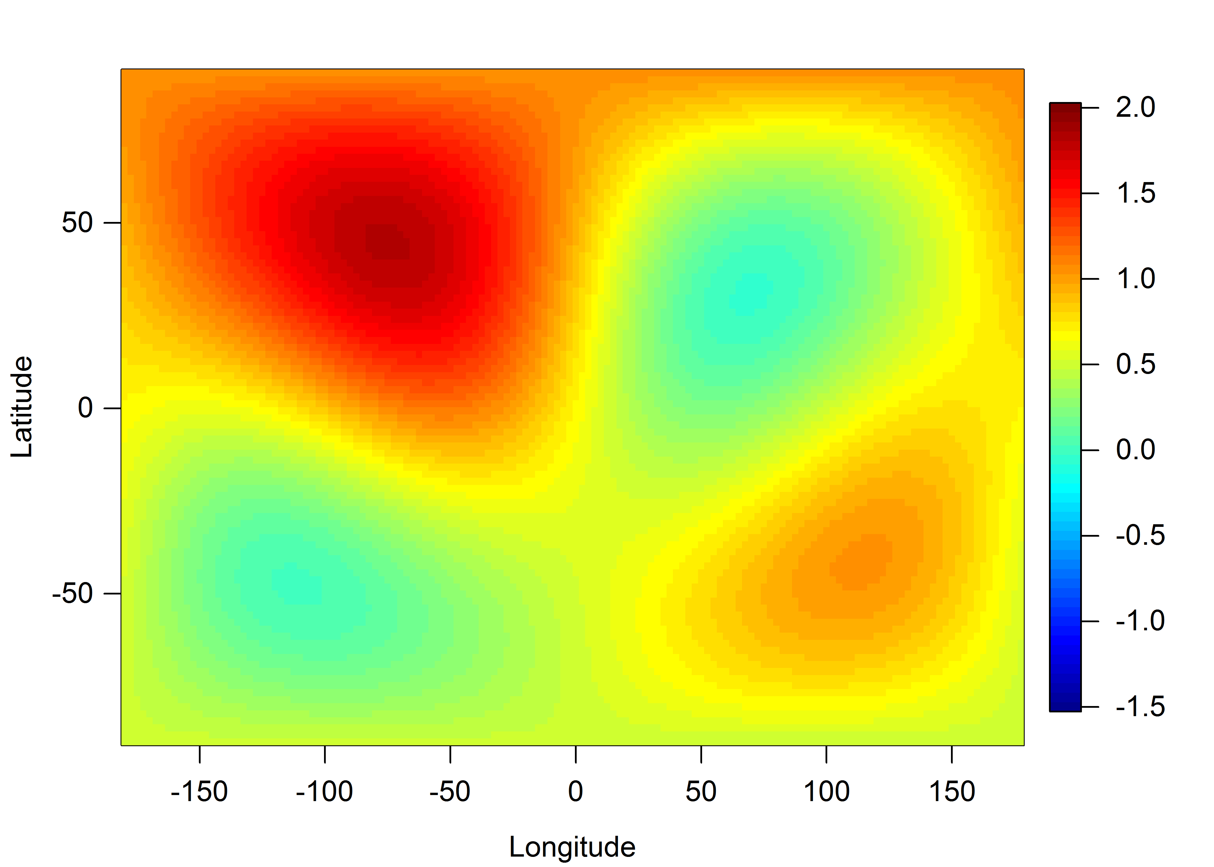
(d) 2nd order $\tau^{F}$

Figure 2: The first 2 order expansion surface for $\kappa^{F}$ and $\tau^{F}$ for observations $y^{F}$.

We provide more illustrations of the flexibility of our approach under various situations: (1) calibration with irregularly spaced outputs over the plane using B-spline basis ; (2) investigation of the connection between the calibration accuracy and the number of computer runs $r$, and between the calibration accuracy and the orders and modes of SHs; (3) comparison of our approach and the empirical orthogonal functions (EOFs) approach and original Kennedy and O’Hagan (2001) framework, in the supplemental material for the interested reader.

4 Application to the WACCM experiments

A series of WACCM runs with the component set prescribed sea ice, data ocean and specified chemistry, with horizontal resolution $1.9\times 2.5^{\circ}$ and 66 vertical levels were simulated from 1st January 2000. The GW parameterizations in WACCM depend on four inputs: (1) cbias ($\theta_{1}\in[-5,5]$): anisotropy of the source spectrum, e.g. -5m/s: the spectrum has a stronger westward component, with center of the spectrum at 5m/s westward. Note that default simulation in WACCM is isotropic (i.e., cbias=0). An anisotropic GW source has been long reckoned to be a potential to improve the middle atmosphere circulation compared to an isotropic source (Medvedev et al., 1998; Hamilton, 2013; Chunchuzov et al., 2015); (2) effgw ($\theta_{2}\in[0.05,0.3]$): the efficiency factor, measures the gravity wave intermittency; (3) flatgw ($\theta_{3}\in[1,3]$): controls the momentum flux of the parameterized waves at the launch levels; (4) launlvl ($\theta_{4}\in[50,700]$): launch levels of the waves. The value of GW inputs $\bm{\theta}$ are generated by a maximin LHD (but scaled to be $[0,1]^{4}$). We simulated $r=100$ runs for 2 months. The first month was discarded as a spin–up period. Each output was computed over 96 latitudes and 144 longitudes, so the total output size is $n\times r=96\times 144\times 100=1382400$. We perform the calibration for the WACCM, either against synthetic (but with added nonstationary observation errors) or real observations, in order to fully validate our approach.

4.1 Calibration against synthetic observations

4.1.1 Model set-up

To illustrate our methodology, we compare the zonal wind simulations $\eta(\mathbf{s}_{i},\bm{\theta}_{j})$, where $\mathbf{s}_{i},i=1,\ldots,96\times 144$ are the latitude and longitude on the spherical domain, and $j=1,\ldots,100$ is the index of the runs, with WACCM’s standard outputs (i.e. default simulation), instead of actual observations. Therefore we know the true GW parameters values and can validate our method. Let $\eta^{\ast}(\mathbf{s}_{i})$ be the zonal wind surface from WACCM standard output. In order to account for possible observation error and lack of physics in the model (discrepancy), and thus evaluate the robustness of our method, we add a smooth noise to $\eta^{\ast}(\mathbf{s}_{i})$ by assuming that the observations are given by:

$$y^{F}(\tilde{\mathbf{s}}_{i})=\eta^{\ast}(\tilde{\mathbf{s}}_{i})+\frac{\sigma_{\eta^{\ast}}}{5}s_{1}+\frac{1}{2}s_{2}s_{3},$$

where $\tilde{\mathbf{s}}_{i}=(s_{1},s_{2},s_{3})$ are the spherical coordinates, and $\sigma_{\eta^{\ast}}=11.14$ is the SD of $\eta^{\ast}$. Fig. 3(a) and (b) shows the zonal wind surfaces from standard outputs and synthetic observations at 30mb, February 2000.

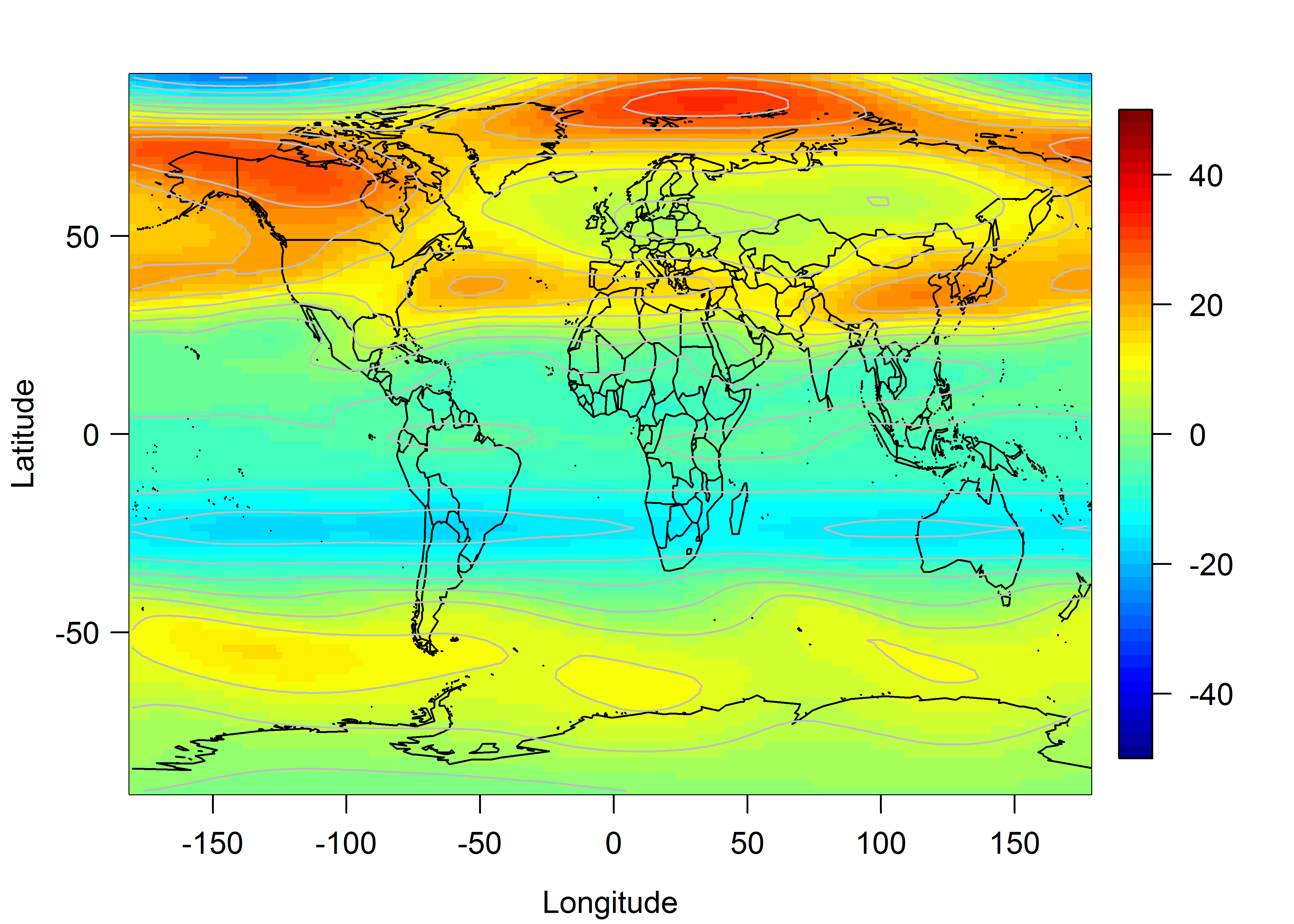
(a) Standard output ($\eta^{\ast}$)

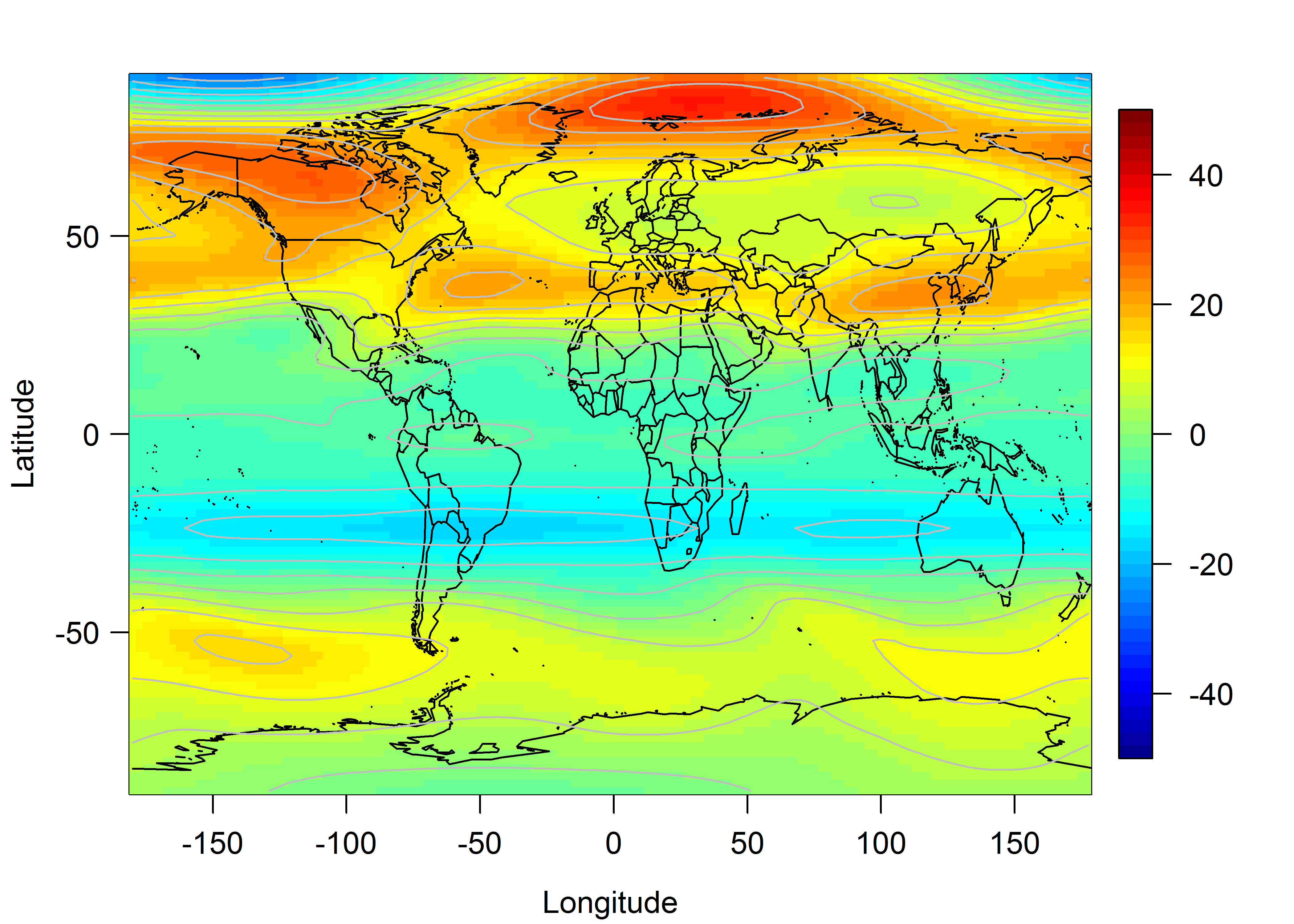
(b) Standard output with noise ($y^{F}$)

Figure 3: (a) Zonal wind standard output; (b) Assumed observed surface: noise and discrepancy added to the zonal wind standard output (30mb, Feb. 2000).

As for the computational issue, in practice it is difficult to deal with a size of model output beyond moderately large (say $\simeq 2000$ responses). Here we have $r=100$ computer runs, therefore we seek to decompose each model output with about 20 coefficients. We represent observations and model discrepancies using 3rd and 4th order SHT for model outputs and observations respectively. This allows enough flexibility. We report two strategies (A) with or (B) without including 1st order SPDE nonstationary information. We also report two other strategies that use (C) 5 or (D) 10 principal components (with 95.8% and 97.9% respectively of the variation explained) to decompose the model outputs and observations (see algorithm in the supplemental material).

Table 2: Posterior mode of GW parameters on the rescaled $[0,1]$ range. Note that the MCMC did not converge in cases C and D, so these estimates are unreliable.

Strategy	cbias	effgw	flatgw	launlvl
	($\theta^{\ast}_{1}=0.5$)	($\theta^{\ast}_{2}=0.56$)	($\theta^{\ast}_{3}=0)$	($\theta^{\ast}_{4}=0.2308$)
A (SH-nonstationary SPDE)	0.435	0.547	0.060	0.276
B (SH-stationary SPDE)	0.361	0.561	0.281	0.282
C (5 PCs)	0.538	0.396	0.741	0.523
D (10 PCs)	0.639	0.082	0.466	0.908

4.1.2 Prediction accuracy

The posterior modes of each strategy are shown in Table 2. Both Strategies A and B calibrate $\theta_{2}$ well and slightly overestimate $\theta_{4}$. The inclusion of SPDE parameters in A v. B not only increases the accuracy of the posterior mode for $\theta_{1}$, but estimate very closely $\theta_{3}$, a difficult task as the true value lies on the lower bound. The quantification of the anisotropic velocity in a large spatial process is a difficult problem (Large et al., 2001; Lauritzen et al., 2015). The improvement of accuracy in the estimation of $\theta_{1}$ confirms the value of using the SPDE technique in the calibration since the nonstationarity allows the amount of flexibility required to identify much clearly the value of $\theta_{1}$.

Unfortunately, the MCMCs do not converge for strategies C and D, hence their posterior modes are uninterpretable (but we report them nevertheless). Note that this result can be expected. Our GW parameterization aims to reduce zonal wind bias at the Tropics associated with the QBO; however, the principal mode of variability in our model outputs occurs across the Northern Hemisphere (in East Asia to be precisely), where the influence of the GW is indirect (see next section for further discussion in comparison with real observations). The PC decomposition will focus on the variability in Northern Hemisphere compared to the Tropics. Recent studies suggest that PC-based approach tends to cause a ‘terminal case analysis’ in the climate modeling (Salter et al., 2018), which means that there is no set of parameters that can allow the model to mimic reality. For this reason the PC-based approach is not appropriate for our calibration setting.

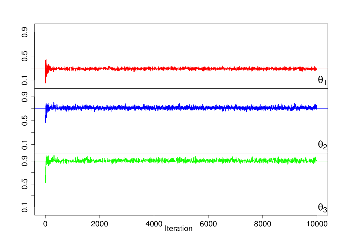
(a) 2nd SHT (9 coefficients)

(b) 9 EOFs representation

Figure 4: MCMC paths of $\bm{\theta}$ for our approach and PC-based algorithms (synthetic case in supplementary material). Solid lines indicate the true values.

Fig. 4 shows a concrete example of such lack of convergence in a synthetic example (see supplementary material). This is a comparison of the MCMC sample paths of the calibration parameters by 2nd order SHs (9 coefficients) and 9 PCs representation. We can see that for all calibration parameters in the SHs approach, convergence occurred after roughly 500 iterations, whereas chains do not converge in the PC approach.

The left panels of Fig. 5 show the boxplots of the marginal posterior distributions for the $\rho_{\eta}$’s for Strategies A and B, which control the dependence strength in each pair of $\bm{\theta}$ in the GP model. The posterior density of $\rho_{4}$ closes to 1 that indicate a very weakly significant effect for $\theta_{4}$. The marginal posterior densities for each $\bm{\theta}$ are displayed in the right panels of Fig. 5. Our approach provides a good compromise between computational feasibility and fidelity to the data by only using parsimonious representations. The results suggest that our technique on calibration of global-scale outputs is effective.

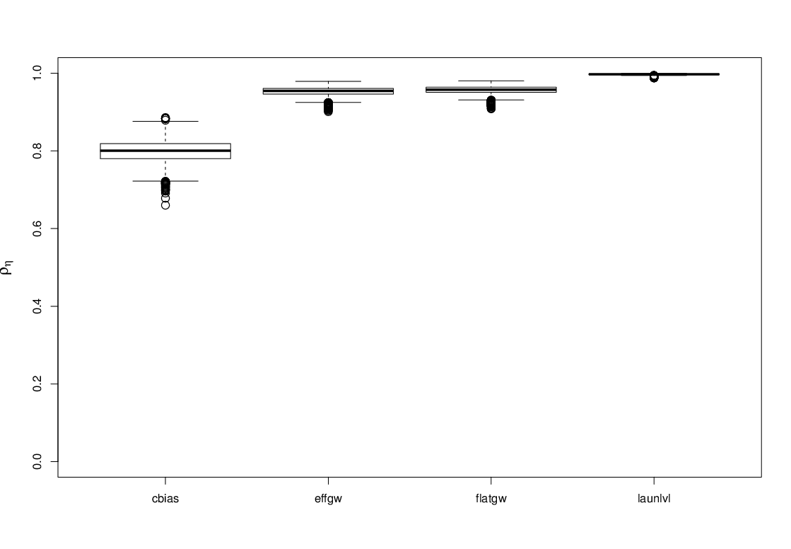
(a) Model A ; $\bm{\rho}_{\eta}$

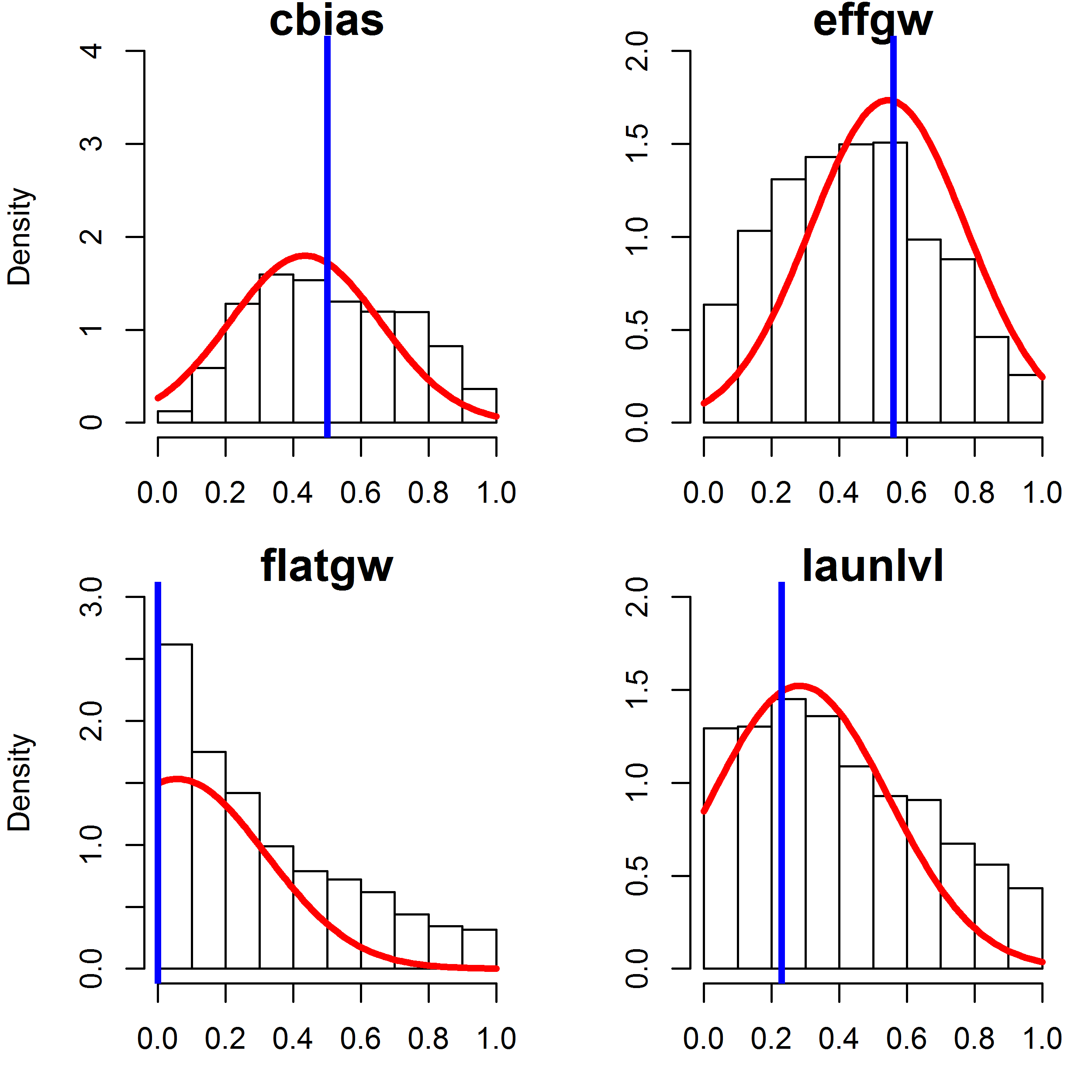
(b) Model A: $\bm{\theta}$

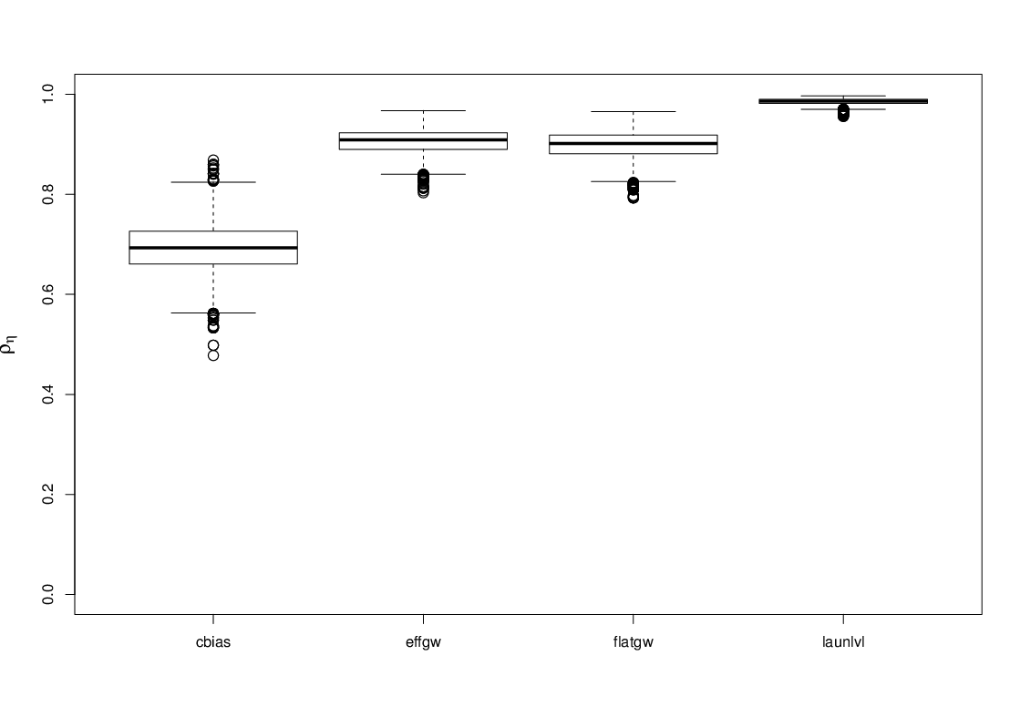
(c) Model B: $\bm{\rho}_{\eta}$

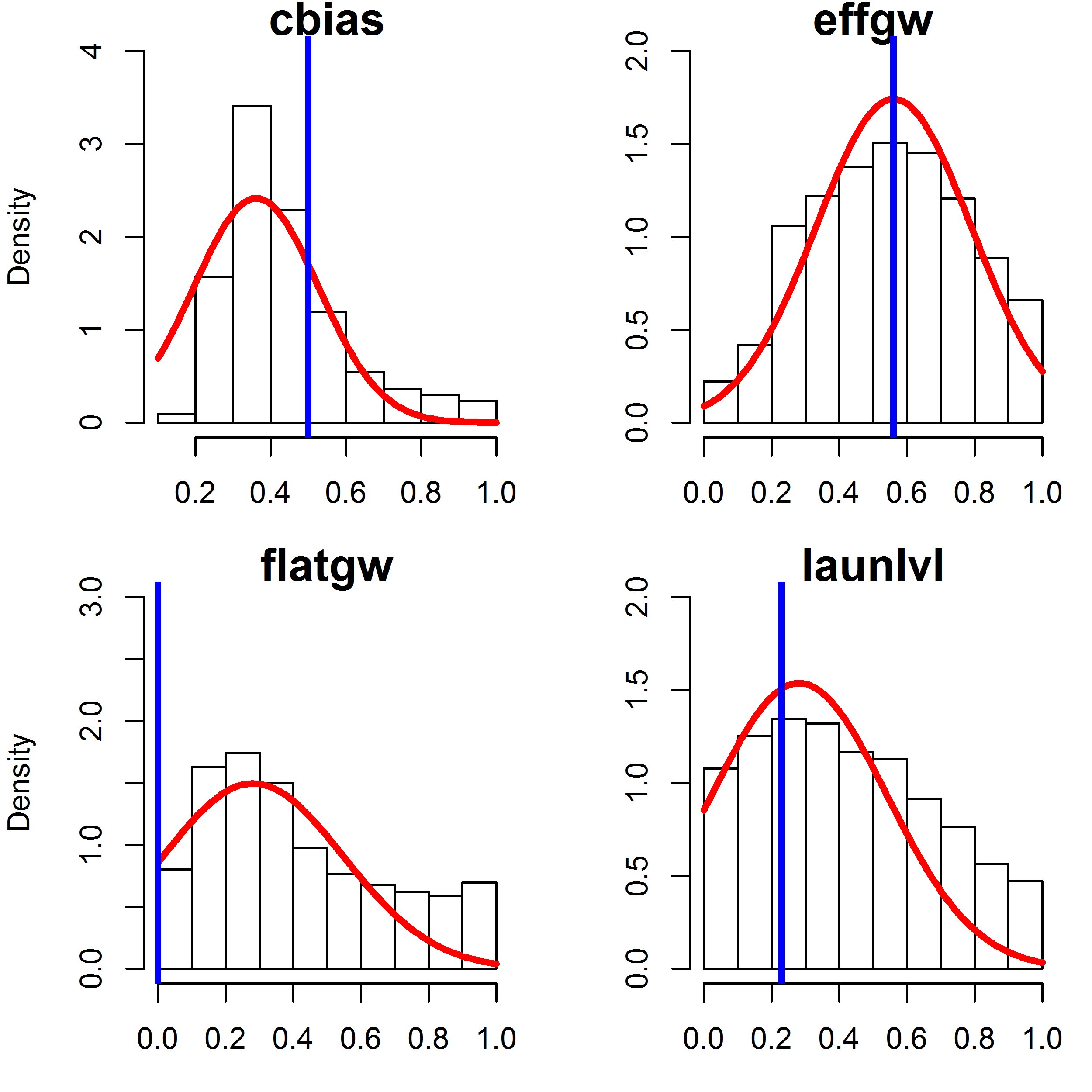
(d) Model B: $\bm{\theta}$

Figure 5: Boxplots of the marginal posterior distribution for correlation parameters $\bm{\rho}_{\eta}$ (left panels); and marginals for the posterior distribution of the GW parameters $\bm{\theta}$ (right panels). Vertical lines indicate the true values (30mb, Feb. 2000).

4.2 Calibration against real observations

4.2.1 Posterior sampling

The final step is to carry out the calibration against real observations. We use zonal wind data obtained from the European Centre for Medium-Range Weather Forecasts (ECMWF) 40 Year Re-analysis (ERA) Data Archive. We focus on the altitude of 1mb, as the outputs in low altitudes are less sensitive to GW parametrizations and match the observations already well. Fig. 6(a) and (b) shows the ERA observations and zonal wind surfaces from standard outputs at 1mb, February 2000. Under the same settings described in the previous section, Fig. 6(c) shows the MCMC paths for 3 chains, with 6000 iterations, corresponding respectively to the calibration parameters. The convergence of the MCMC chain can be established for the parameters $\theta_{2}$, $\theta_{3}$ and $\theta_{4}$, with posterior modes 0.107 (SD=0.051), 0.081 (SD=0.029) and 0.339 (SD=0.018) in the $[0,1]$ scale, respectively. The posterior mode of $\theta_{1}$ lies in upper bound. We then use posterior modes for these paths, collected as input values for the validation of WACCM. The calibrated output displayed in Fig. 6(d), shown a root-mean-square error (RMSE) of 18.15, which is a percentage of improvement of 14.99% over the standard output (the RMSE between ERA observations and standard output is 21.35).

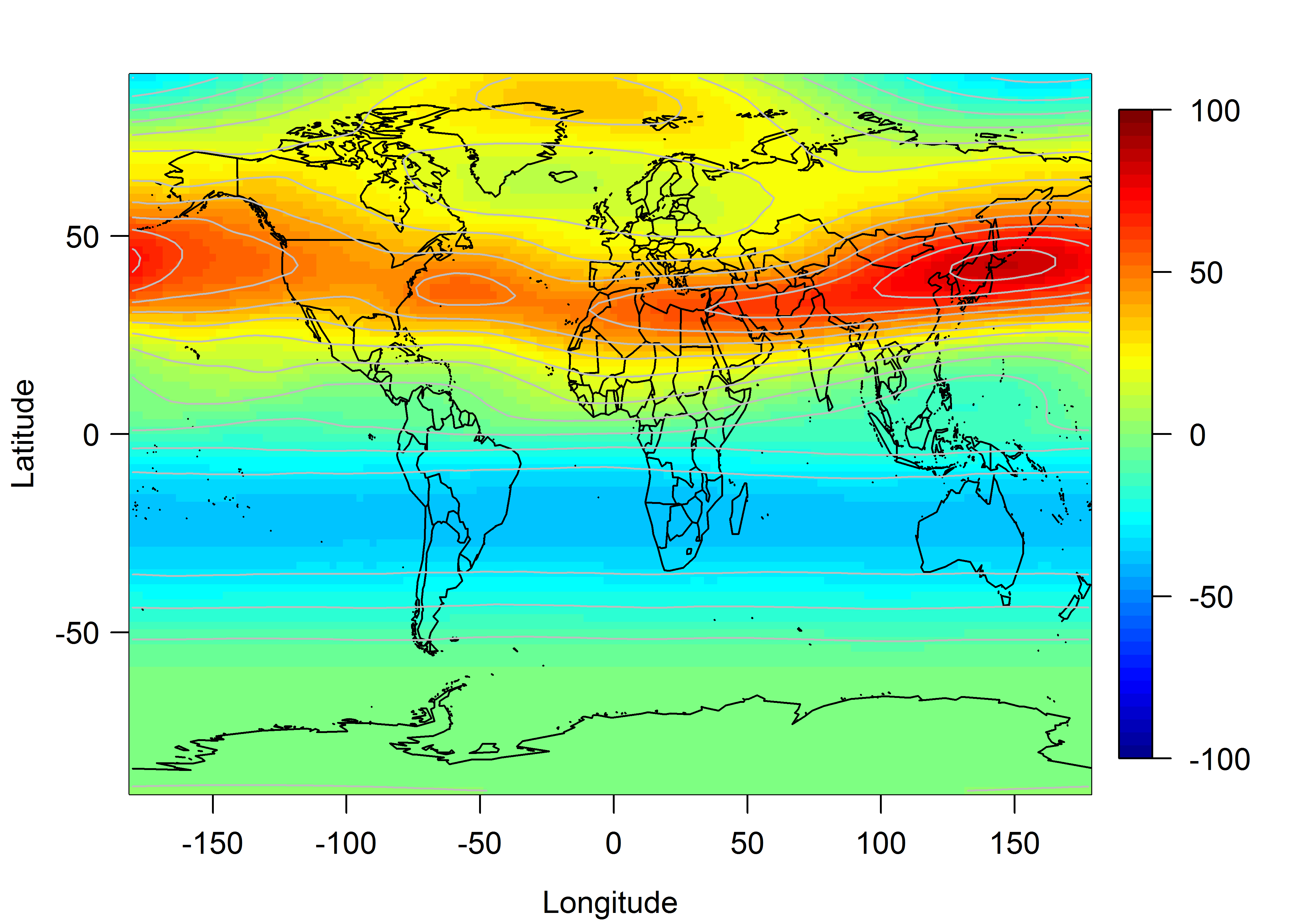
(a) ERA obs.

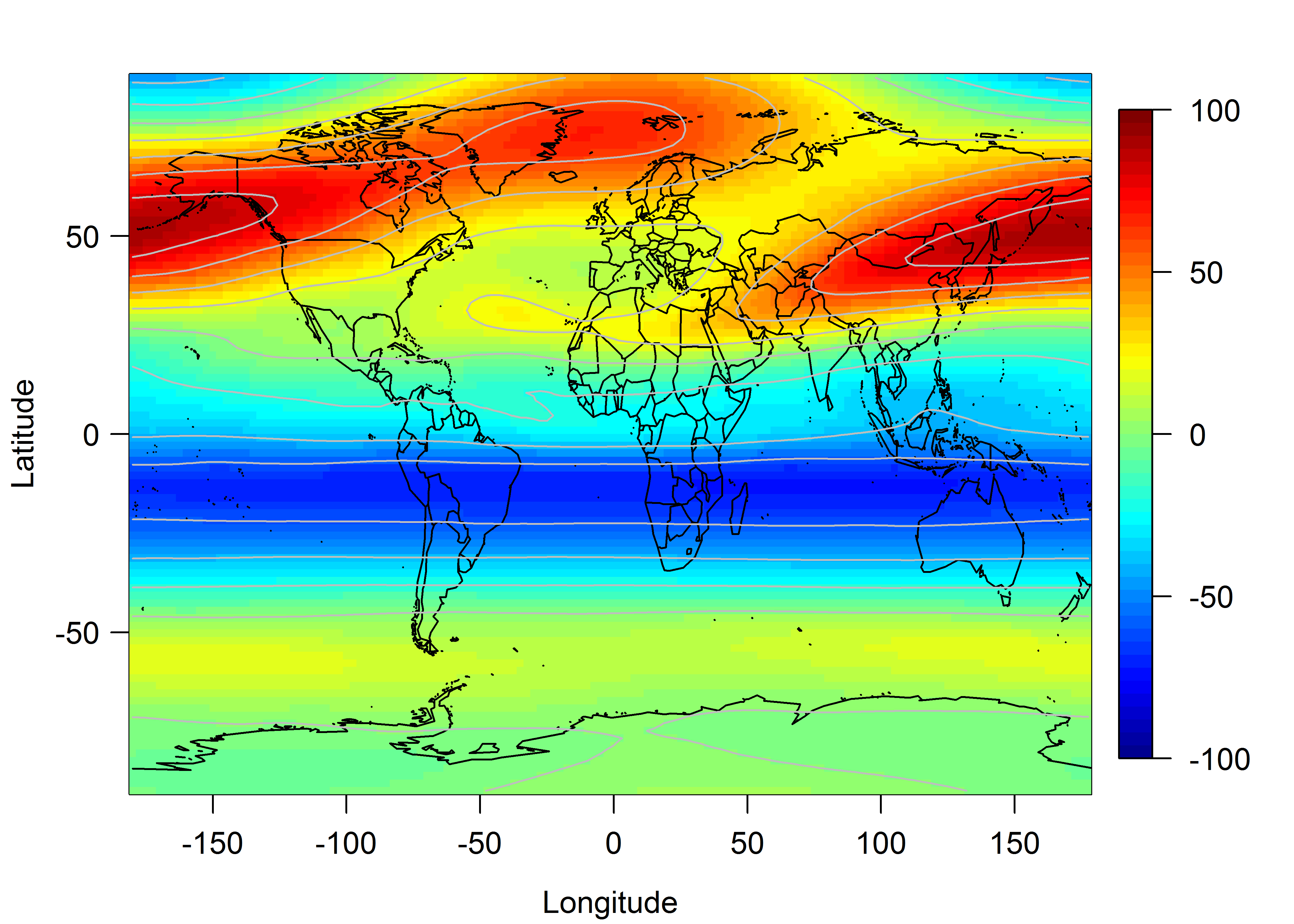
(b) Standard output

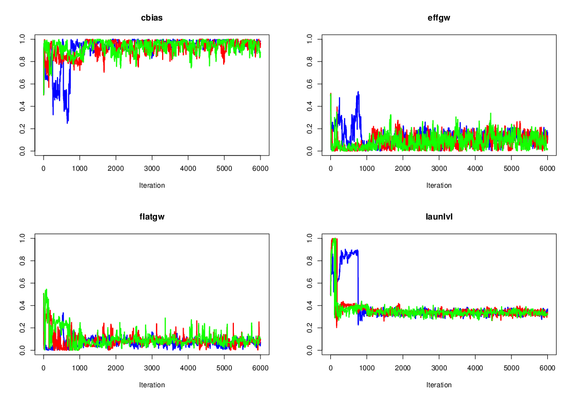
(c) MCMC paths

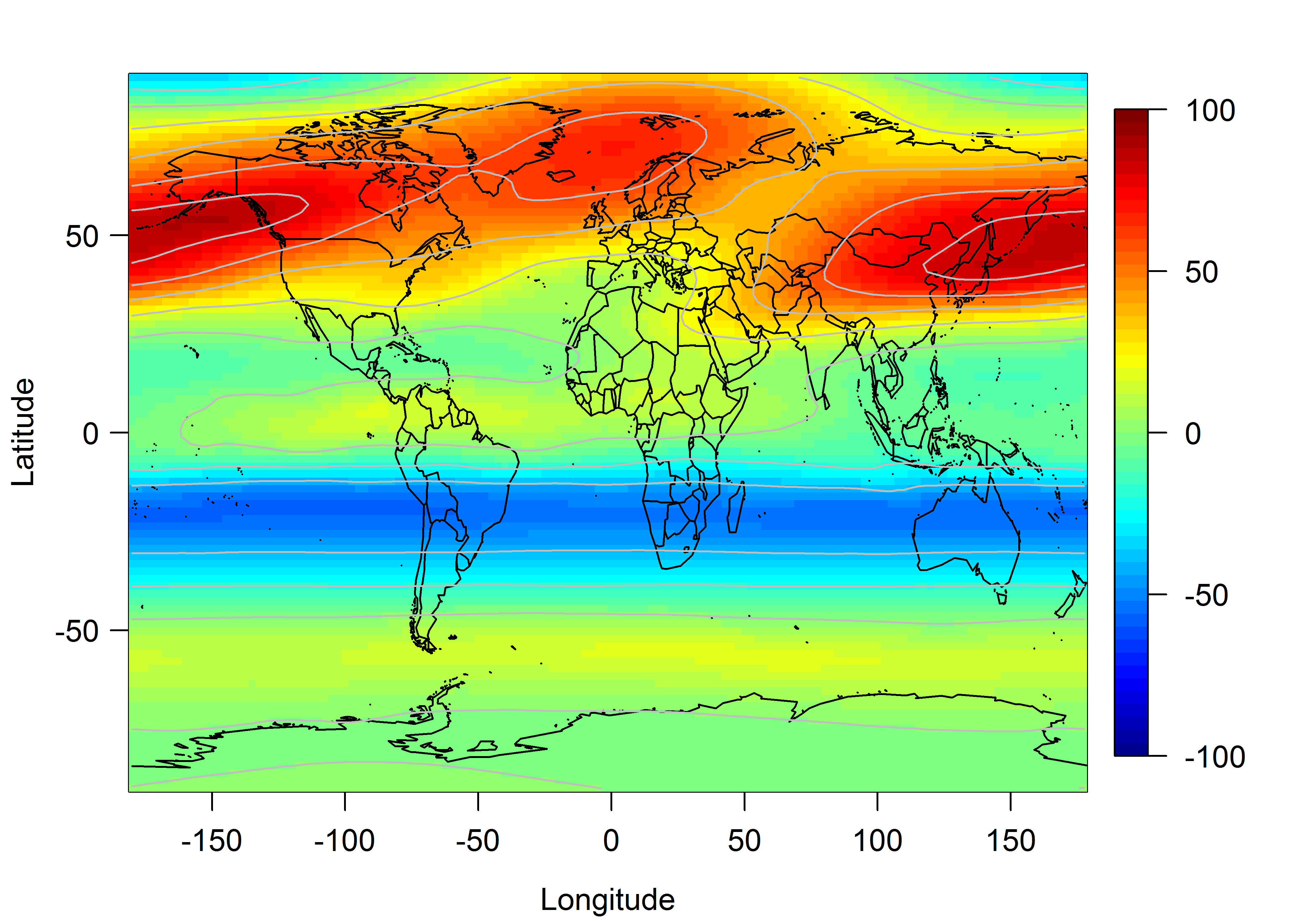
(d) Calibrated output

Figure 6: Zonal wind from the (a) ERA data and (b) WACCM standard output; (c) MCMC paths for 3 chains and (d) Zonal wind generated by posterior from the calibration (1mb, Feb. 2000).

The resulting histograms for the calibration parameters, with first 1000 iterations dropped as they are reckoned to be in burn-in, are shown in Fig. 7. As expected from MCMC plot, a normal distribution can be established for $\theta_{2}$, $\theta_{3}$ and $\theta_{4}$. The distribution of $\theta_{1}$ shows is skewed against the upper bound. It means that the possible calibrated value may lie outside the boundary. Since $\theta_{1}$ represents the anisotropic velocity of zonal wind (the model default is assumed to be isotropic), the results suggest that we would need a more eastward component. It seems that this is a spurious effect of the simplicity in the parameterization. Indeed, in order to avoid losing the westward components and to acknowledge the physical reality, it may be helpful to have a “bi-modal" spectrum (Arfeuille et al., 2013; Zhu et al., 2017), with one peak in the eastward direction and another in the westward, and these two components do not have to be the same. Indeed, uneven amplitudes of the QBO easterly and westerly phases are often observed in the previous studies (Naujokat, 1986; Garcia et al., 1997; Ern et al., 2008). GWs schemes are currently under development within the NCAR WACCM working group to improve the representation of the QBO and help fix the cold pole problem (Garcia et al., 2017). Further development will allow us to have more flexible GWs schemes, but it is beyond the scope of the present setting for the climate simulation.

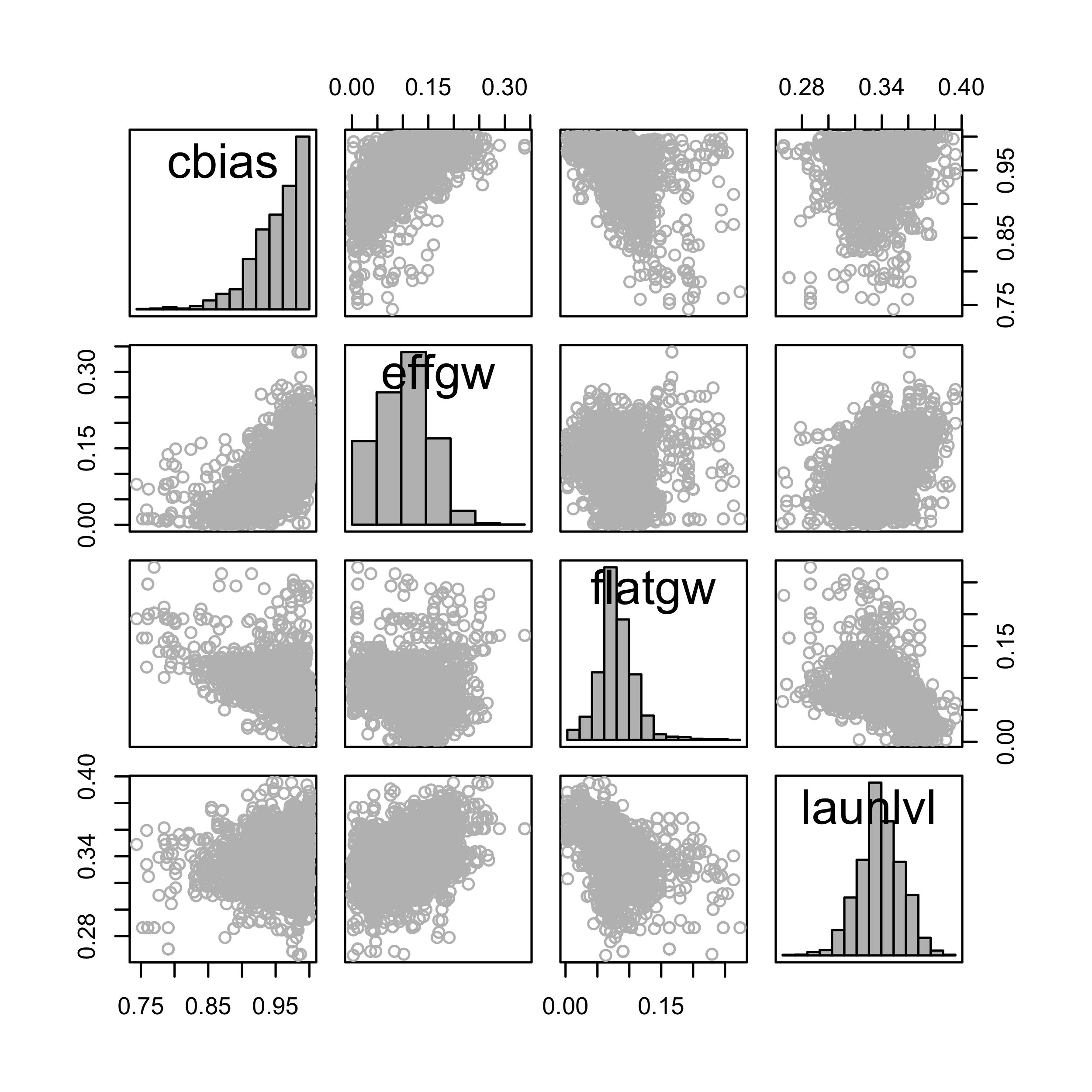
Figure 7: Density of posterior calibration parameter for zonal wind simulation (1mb, Feb. 2000).

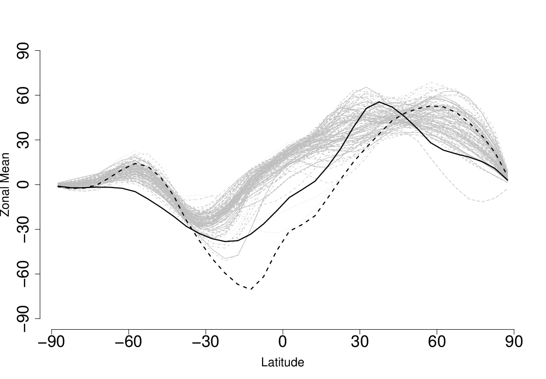
(a) Zonal means

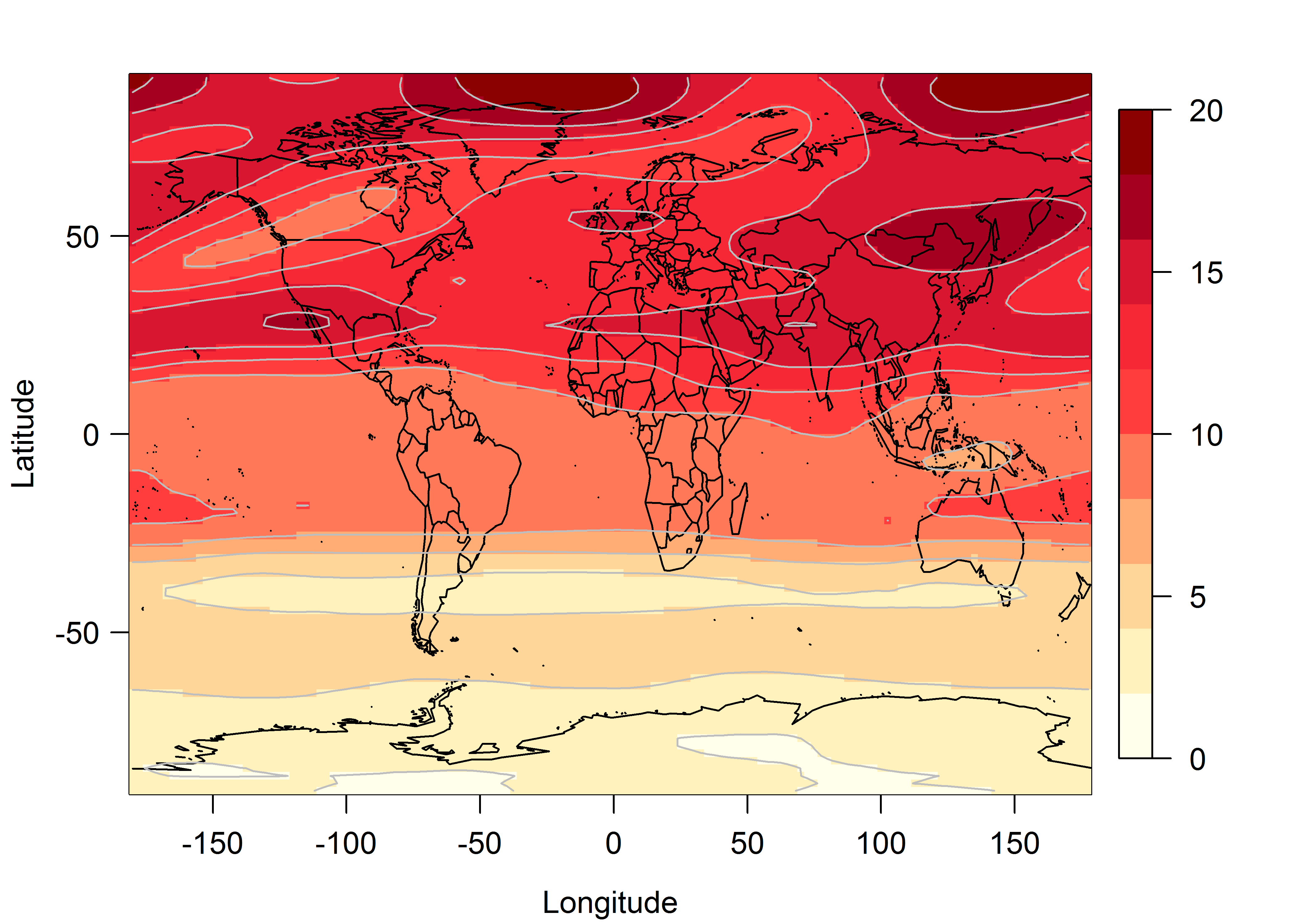
(b) Grid-by-grid SDs

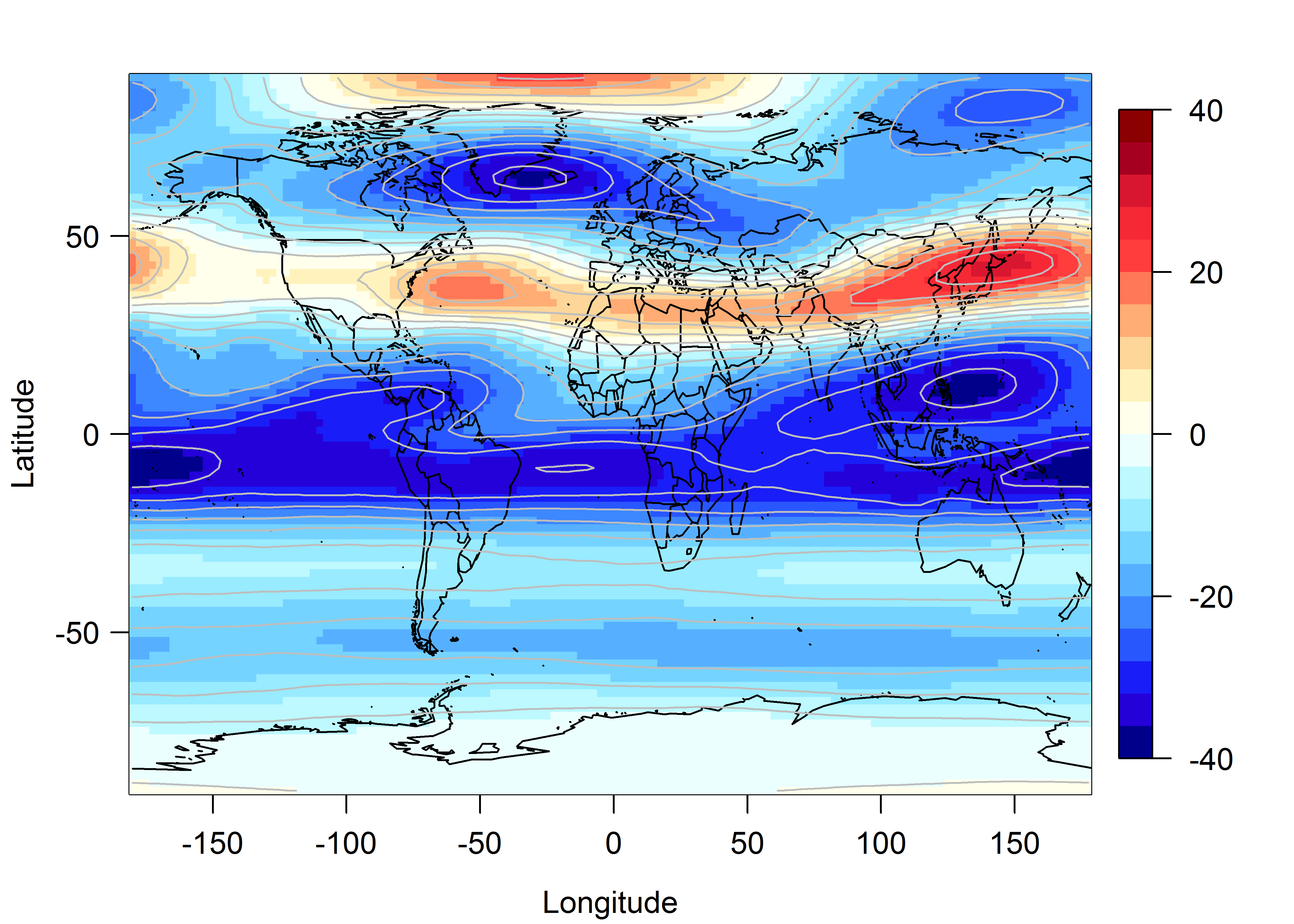
(c) Grid-by-grid differences

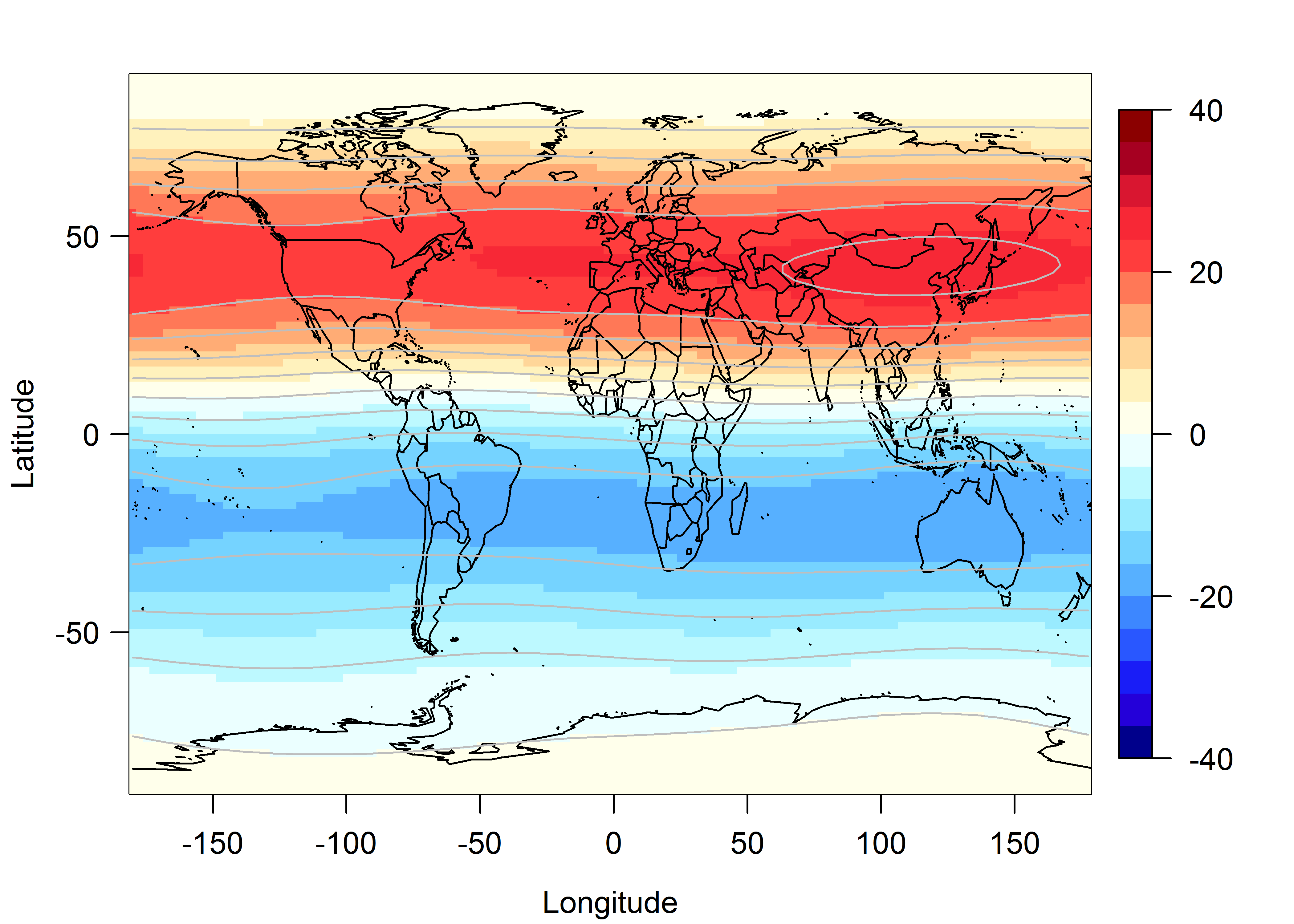
(d) Model mean discrepancies

Figure 8: (a) Zonal means of observations (black solid line), standard (black dashed line) and model outputs (grey dotted lines); (b) Grid-by-Grid SDs map across model runs; (c) Differences between observations and mean structure of model outputs and (d) Model mean discrepancies map (1mb, Feb. 2000).

4.2.2 Model discrepancy and uncertainty

In order to assess the model uncertainty, Fig. 8(a) shows the zonal means calculated over every $5^{\circ}$ belt of observations (black solid line), standard outputs (black dashed line) and each run of model output (grey dotted lines): note that the zonal means over the Tropics are high compared to the observations and standard outputs. The input value of $\theta_{3}$ in the standard output is being at the lower border of parameter range, this may produce relatively extreme behavior over the Tropics in our model runs. Fig. 8(b) represents the grid-by-grid SDs map across model outputs. We can see that the spatial process is clearly anisotropic and highly latitude dependent; the uncertainties are concentrated over the Northern Hemisphere, and little significant variabilities can be found over the Southern Hemisphere. Fig. 8(c) compares the differences between observations and mean structure of model outputs in each cell (with respect to 100 LHD), i.e. $\delta_{\text{initial}}(\mathbf{s})=y^{F}(\mathbf{s})-\bar{\eta}(\mathbf{s},\bm{\theta})$, where $\bar{\eta}(\mathbf{s})$ is the output means over space. This figure provides potential features of model discrepancy over space (albeit not the true discrepancy). As expected, the model tends to overestimate the values over the Tropics, which matches the pattern in Fig. 8(a). Besides, this surface seems to match the pattern in Fig. 8(b). The largest model bias (apart from the Tropics) and variability both occur over Northeast Asia and the North Pole. Fig. 8(d) shows the posterior mean discrepancies surface in the sense of $\delta^{\ast}(\mathbf{s})=y^{R}(\mathbf{s})-\eta(\mathbf{s},\bm{\theta}^{\ast})$. Our calibration reduces the bias (i.e. overestimation) over the Tropics, as well as the bias (i.e. underestimation) over the North Pole, whereas the bias over the Northeast Asia remains.

4.2.3 Validation

We use the mode from each posterior distribution to simulate 5 years (2 QBO cycles) of zonal wind output. Fig. 9(a) shows monthly RMSEs at 1mb globally, from 2000 to 2004. The overall averaged RMSE for the standard and calibrated outputs are 24.51 and 22.99, respectively, a small improvement. Indeed, our inertial GW scheme is designed to reduce the zonal wind bias over Tropics, we should not expect that our calibration will improve model simulations globally. We thus investigate RMSEs over the Tropics over the same period. The RMSE trends are shown in Fig. 9(b). The overall averaged RMSE over the Tropics for the standard and calibrated outputs are 26.64 and 17.87, respectively. Therefore the improvement is more significant over the Tropics, with percentage of improvement 32.9%. Simulations by our calibrated outputs outperform the standard code in 51 months out of 60 months. The calibration of WACCM with real observations over the whole output domain (i.e. including across altitudes) constitutes another level of complexity that needs joint scientific and statistical expertise. It is currently under investigation, but is beyond the scope of this paper. Indeed, observations are scarce at these altitudes and show features that require specific understanding of the upper atmosphere dynamics before being used for calibration, and over many years of simulation for an adequate comparison.

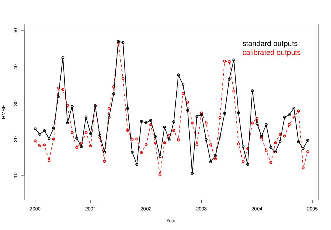
(a) Global RMSEs

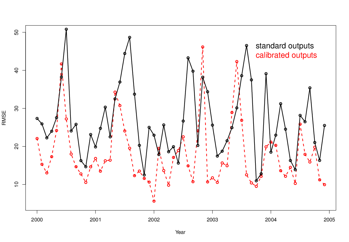
(b) Tropical RMSEs

Figure 9: Monthly RMSE trends between the ERA observations and standard outputs (solid line) or calibrated outputs (dashed line), from 2000 to 2004.

5 Conclusion and discussion

Our approach improved the calibration of large–scale computer model outputs distributed over spaces, parsimoniously, by using bases representations for the mean structures of the spatial surfaces. In addition, the INLA–SPDE approach was used to decompose its parameters characterizing nonstationarity over the the same bases in order to improve calibration. The synthetic and real examples confirm the ability of our approach to efficiently and accurately perform calibration. Our method was inspired by the wavelets method of Bayarri et al. (2007), but with a different type of outputs: spatial v. time series. We can expect that the spherical wavelet decomposition may also be a possible alternative basis representation on the spatial domain, whenever appropriate (e.g. for sharp variations).

Another advantage of using the SH basis, compared to data-driven ones such as PCs, is that sequential design is allowed (Beck and Guillas, 2016), because the basis elements will not change, and model runs are obtained at the same grids or scattered locations. In this study we illustrate our technique to a specific horizontal output from the WACCM simulator. The SHT of model outputs can also be extended to time varying processes. As noted by Jones (1963), if a random field on a sphere varies with time, the representation becomes $\eta(\mathbf{s},t)=\sum_{k=0}^{\infty}\sum_{h=-k}^{k}c_{k,h}(t)\psi_{k,h}(\mathbf{s})$, where $c_{k,h}(t)$ being an ordinary one-dimensional stochastic process. The set of all $c_{k,h}(t)$ form an infinite dimensional stochastic process. Theoretically we can represent model outputs in space–time settings with such representations. Nevertheless, in climate or chemistry–transport simulations, we often encounter not only outputs in time and horizontal resolution, but also in vertical resolution. Therefore extensions to 4 dimensional correlations are needed, but they must maintain the computational tractability.

In our approach the covariance matrix is formulated as a block diagonal structure. We could relax this assumption and then adopt the block composite likelihood approach to accelerate the algorithm (Chang et al., 2015b). Unfortunately, this approach only cover the stationary case (though could be extended). Our approach naturally and efficiently models nonstationarity in space. Furthermore, there are cases where our approach is computationally more efficient than Chang et al. (2015b). Indeed, if $m$ is large, their computational cost is about $O(\sum_{i=1}^{B}m_{i}^{3})$, where $\sum_{i=1}^{B}m_{i}=m$ (depends on number and size of blocks $m_{i}$), whereas our cost is $O(N^{3}_{y}r^{3})$, which is lower in many, but not all, applications. Since our climate experiment involves direct input-output projection, another potential extension of our approach is to combine recent development on Bayesian treed calibration technique, which partitions input space into subregions where our reduced rank approach can be applied, to further accelerate the calibration (Karagiannis et al., 2017; Konomi et al., 2017).

References

- Alexander et al. (2010) Alexander, M. J., Geller, M., McLandress, C., Polavarapu, S., Preusse, P., Sassi, F., Sato, K., Eckermann, S., Ern, M., Hertzog, A., Kawatani, Y., Pulido, M., Shaw, T. A., Sigmond, M., Vincent, R., and Watanabe, S. (2010). Recent developments in gravity-wave effects in climate models and the global distribution of gravity-wave momentum flux from observations and models. Q. J. R. Meteorol. Soc., 136(650):1103–1124.
- Alexander and Sato (2015) Alexander, M. J. and Sato, K. (2015). Gravity wave dynamics and climate: an update from the SPARC gravity wave activity. SPARC newslett., 44(44):9–13.
- Arfeuille et al. (2013) Arfeuille, F., Luo, B., Heckendorn, P., Weisenstein, D., Sheng, J., Rozanov, E., Schraner, M., Brönnimann, S., Thomason, L., and Peter, T. (2013). Modeling the stratospheric warming following the Mt. Pinatubo eruption: uncertainties in aerosol extinctions. Atmos. Chem. phys., 13(22):11221–11234.
- Banerjee et al. (2008) Banerjee, S., Gelfand, A. E., Finley, A. O., and Sang, H. (2008). Gaussian predictive process models for large spatial data sets. J. R. Statist. Soc. B, 70(4):825–848.
- Bayarri et al. (2007) Bayarri, M., Berger, J., Cafeo, J., Garcia-Donato, G., Liu, F., Palomo, J., Parthasarathy, R., Paulo, R., Sacks, J., and Walsh, D. (2007). Computer model validation with functional output. Ann. Statist., 35(5):1874–1906.
- Beck and Guillas (2016) Beck, J. and Guillas, S. (2016). Sequential design with mutual information for computer experiments (MICE): emulation of a tsunami model. J. Uncertnty Quant., 4(1):739–766.
- Bhat et al. (2010) Bhat, K. S., Haran, M., and Goes, M. (2010). Computer model calibration with multivariate spatial output: A case study. In Chen, M.-H., Dey, D. K., Müller, P., Sun, D., and Ye, K., editors, Frontiers of Statistical Decision Making and Bayesian Analysis, pages 168–184. Springer New York.
- Blangiardo and Cameletti (2015) Blangiardo, M. and Cameletti, M. (2015). Spatial and spatio-temporal Bayesian models with R-INLA. John Wiley & Sons.
- Bolin and Lindgren (2011) Bolin, D. and Lindgren, F. (2011). Spatial models generated by nested stochastic partial differential equations, with an application to global ozone mapping. Ann. Appl. Statist., 5(1):523–550.
- Bowman and Woods (2016) Bowman, V. E. and Woods, D. C. (2016). Emulation of multivariate simulators using thin-plate splines with application to atmospheric dispersion. J. Uncertnty Quant., 4(1):1323–1344.
- Brynjarsdóttir and O’Hagan (2014) Brynjarsdóttir, J. and O’Hagan, A. (2014). Learning about physical parameters: The importance of model discrepancy. Inv. Probl., 30(11):114007 (24pp).
- Cameletti et al. (2013) Cameletti, M., Lindgren, F., Simpson, D., and Rue, H. (2013). Spatio-temporal modeling of particulate matter concentration through the SPDE approach. Adv. Statist. Anal., 97(2):109–131.
- Chakraborty et al. (2013) Chakraborty, A., Mallick, B. K., Mcclarren, R. G., Kuranz, C. C., Bingham, D., Grosskopf, M. J., Rutter, E. M., Stripling, H. F., and Drake, R. P. (2013). Spline-based emulators for radiative shock experiments with measurement error. J. Am. Statist. Ass., 108(502):411–428.
- Chang et al. (2015a) Chang, K.-L., Guillas, S., and Fioletov, V. E. (2015a). Spatial mapping of ground-based observations of total ozone. Atmos. Measmnt Tech., 8(10):4487–4505.
- Chang et al. (2017) Chang, K.-L., Petropavlovskikh, I., Cooper, O. R., Schultz, M. G., and Wang, T. (2017). Regional trend analysis of surface ozone observations from monitoring networks in eastern North America, Europe and East Asia. Elem. Sci. Anth., 5(50):1–22.
- Chang et al. (2014) Chang, W., Haran, M., Olson, R., and Keller, K. (2014). Fast dimension-reduced climate model calibration and the effect of data aggregation. Ann. Appl. Statist., 8(2):649–673.
- Chang et al. (2015b) Chang, W., Haran, M., Olson, R., and Keller, K. (2015b). A composite likelihood approach to computer model calibration with high-dimensional spatial data. Statist. Sin., 25:243–259.
- Chunchuzov et al. (2015) Chunchuzov, I., Kulichkov, S., Perepelkin, V., Popov, O., Firstov, P., Assink, J., and Marchetti, E. (2015). Study of the wind velocity-layered structure in the stratosphere, mesosphere, and lower thermosphere by using infrasound probing of the atmosphere. J. Geophys. Res. Atmos., 120(17):8828–8840.
- Cressie and Johannesson (2008) Cressie, N. and Johannesson, G. (2008). Fixed rank kriging for very large spatial data sets. J. R. Statist. Soc. B, 70(1):209–226.
- Ern et al. (2014) Ern, M., Ploeger, F., Preusse, P., Gille, J., Gray, L., Kalisch, S., Mlynczak, M., Russell, J., and Riese, M. (2014). Interaction of gravity waves with the QBO: A satellite perspective. J. Geophys. Res. Atmos., 119(5):2329–2355.
- Ern et al. (2008) Ern, M., Preusse, P., Krebsbach, M., Mlynczak, M., and Iii, J. R. (2008). Equatorial wave analysis from SABER and ECMWF temperatures. Atmos. Chem. Phys., 8(4):845–869.
- Fuglstad et al. (2015) Fuglstad, G.-A., Lindgren, F., Simpson, D., and Rue, H. (2015). Exploring a new class of non-stationary spatial Gaussian random fields with varying local anisotropy. Statist. Sin., pages 115–133.
- Furrer and Sain (2009) Furrer, R. and Sain, S. R. (2009). Spatial model fitting for large datasets with applications to climate and microarray problems. Statist. Comput., 19(2):113–128.
- Garcia et al. (1997) Garcia, R. R., Dunkerton, T. J., Lieberman, R. S., and Vincent, R. A. (1997). Climatology of the semiannual oscillation of the tropical middle atmosphere. J. Geophys. Res. Atmos., 102(D22):26019–26032.
- Garcia et al. (2017) Garcia, R. R., Smith, A. K., Kinnison, D. E., Cámara, D. L. Á., and Murphy, D. J. (2017). Modification of the gravity wave parameterization in the Whole Atmosphere Community Climate Model: Motivation and results. J. Atmos. Sci., 74(1):275–291.
- Geller et al. (2013) Geller, M. A., Alexander, M. J., Love, P. T., Bacmeister, J., Ern, M., Hertzog, A., Manzini, E., Preusse, P., Sato, K., Scaife, A. A., and Zhou, T. (2013). A comparison between gravity wave momentum fluxes in observations and climate models. J. Clim., 26(17):6383–6405.
- Genton and Kleiber (2015) Genton, M. G. and Kleiber, W. (2015). Cross-covariance functions for multivariate geostatistics. Statist. Sci., 30(2):147–163.
- Gneiting (2013) Gneiting, T. (2013). Strictly and non-strictly positive definite functions on spheres. Bernoulli, 19(4):1327–1349.
- Gneiting et al. (2010) Gneiting, T., Kleiber, W., and Schlather, M. (2010). Matérn cross-covariance functions for multivariate random fields. J. Am. Statist. Ass., 105(491):1167–1177.
- Gramacy and Apley (2015) Gramacy, R. B. and Apley, D. W. (2015). Local Gaussian process approximation for large computer experiments. J. Computatnl. Graph. Statist., 24(2):561–578.
- Hamilton (2013) Hamilton, K. (2013). Gravity wave processes: their parameterization in global climate models, volume 50. Springer Science & Business Media.
- Higdon et al. (2008) Higdon, D. M., Gattiker, J. R., Williams, B., and Rightley, M. (2008). Computer model calibration using high dimensional output. J. Am. Statist. Ass., 103:570–583.
- Higdon et al. (2004) Higdon, D. M., Kennedy, M., Cavendish, J. C., Cafeo, J. A., and Ryne, R. D. (2004). Combining field data and computer simulations for calibration and prediction. SIAM J. Scient. Comput., 26(2):448–466.
- Holden et al. (2015) Holden, P. B., Edwards, N. R., Garthwaite, P. H., and Wilkinson, R. D. (2015). Emulation and interpretation of high-dimensional climate model outputs. J. Appl. Statist., 42(9):2038–2055.
- Ilyas et al. (2017) Ilyas, M., Brierley, C. M., and Guillas, S. (2017). Uncertainty in regional temperatures inferred from sparse global observations: Application to a probabilistic classification of El Niño. Geophys. Res. Lett., 44(17):9068–9074.
- Jones (1963) Jones, R. H. (1963). Stochastic processes on a sphere. Ann. Math. Statist., 34:213–218.
- Jun et al. (2008) Jun, M., Knutti, R., and Nychka, D. W. (2008). Spatial analysis to quantify numerical model bias and dependence: how many climate models are there? J. Am. Statist. Ass., 103(483):934–947.
- Jun and Stein (2007) Jun, M. and Stein, M. L. (2007). An approach to producing space–time covariance functions on spheres. Technometrics, 49(4):468–479.
- Jun and Stein (2008) Jun, M. and Stein, M. L. (2008). Nonstationary covariance models for global data. Ann. Appl. Statist., 2:1271–1289.
- Karagiannis et al. (2017) Karagiannis, G., Konomi, B. A., and Lin, G. (2017). On the Bayesian calibration of expensive computer models with input dependent parameters. Spatl Statist., In press.
- Katzfuss and Cressie (2011) Katzfuss, M. and Cressie, N. (2011). Spatio-temporal smoothing and EM estimation for massive remote-sensing data sets. J. Time Ser. Anal., 32(4):430–446.
- Kennedy and O’Hagan (2001) Kennedy, M. and O’Hagan, A. (2001). Bayesian calibration of computer models. J. R. Statist. Soc. B, 63:425–464.
- Kleiber and Nychka (2012) Kleiber, W. and Nychka, D. W. (2012). Nonstationary modeling for multivariate spatial processes. J, Multiv. Anal., 112:76–91.
- Konomi et al. (2017) Konomi, B. A., Karagiannis, G., Lai, K., and Lin, G. (2017). Bayesian Treed Calibration: an application to carbon capture with AX sorbent. J. Am. Statist. Ass., 112(517):37–53.
- Lamarque et al. (2013) Lamarque, J.-F., Shindell, D. T., Josse, B., Young, P. J., Cionni, I., Eyring, V., Bergmann, D., Cameron-Smith, P., Collins, W. J., Doherty, R., Dalsoren, S., Faluvegi, G., Folberth, G., Ghan, S. J., Horowitz, L. W., Lee, Y. H., MacKenzie, I. A., Nagashima, T., Naik, V., Plummer, D., Righi, M., Rumbold, S. T., Schulz, M., Skeie, R. B., Stevenson, D. S., Strode, S., Sudo, K., Szopa, S., Voulgarakis, A., and Zeng, G. (2013). The Atmospheric Chemistry and Climate Model Intercomparison Project (ACCMIP): overview and description of models, simulations and climate diagnostics. Geoscient. Modl Devlpmnt, 6:179–206.
- Large et al. (2001) Large, W. G., Danabasoglu, G., McWilliams, J. C., Gent, P. R., and Bryan, F. O. (2001). Equatorial circulation of a global ocean climate model with anisotropic horizontal viscosity. J. Phys. Oceanog., 31(2):518–536.
- Lauritzen et al. (2015) Lauritzen, P. H., Bacmeister, J. T., Callaghan, P. F., and Taylor, M. A. (2015). NCAR global model topography generation software for unstructured grids. Geoscient. Modl Devlpmnt, 8(6):3975–3986.
- Lindgren and Rue (2015) Lindgren, F. and Rue, H. (2015). Bayesian spatial and spatiotemporal modelling with R-INLA. J. Statist. Softwr., 63(19):1–25.
- Lindgren et al. (2011) Lindgren, F., Rue, H., and Lindström, J. (2011). An explicit link between Gaussian fields and Gaussian Markov random fields: the stochastic partial differential equation approach. J. R. Statist. Soc. B, 73(4):423–498.
- Linkletter et al. (2006) Linkletter, C., Bingham, D., Hengartner, N., Higdon, D. M., and Ye, K. Q. (2006). Variable selection for Gaussian process models in computer experiments. Technometrics, 48(4):478–490.
- Liu et al. (2014) Liu, H., McInerney, J., Santos, S., Lauritzen, P., Taylor, M., and Pedatella, N. (2014). Gravity waves simulated by high-resolution Whole Atmosphere Community Climate Model. Geophy. Res. Lett., 41(24):9106–9112.
- Liu et al. (2009) Liu, H., Sassi, F., and Garcia, R. (2009). Error growth in a whole atmosphere climate model. J. Atmos. Sci., 66(1):173–186.
- Liu et al. (2016) Liu, X., Guillas, S., and Lai, M.-J. (2016). Efficient spatial modeling using the SPDE approach with bivariate splines. J. Computnl. Graph. Statist., 25(4):1176–1194.
- Medvedev et al. (1998) Medvedev, A., Klaassen, G., and Beagley, S. (1998). On the role of an anisotropic gravity wave spectrum in maintaining the circulation of the middle atmosphere. Geophys. Res. Lett., 25(4):509–512.
- Muir and Tkalčić (2015) Muir, J. and Tkalčić, H. (2015). A method of spherical harmonic analysis in the geosciences via hierarchical Bayesian inference. Geophys. J. Int., 203(2):1164–1171.
- Naujokat (1986) Naujokat, B. (1986). An update of the observed quasi-biennial oscillation of the stratospheric winds over the tropics. J. Atmos. Sci., 43(17):1873–1877.
- Nychka et al. (2015) Nychka, D. W., Bandyopadhyay, S., Hammerling, D., Lindgren, F., and Sain, S. (2015). A multiresolution Gaussian process model for the analysis of large spatial datasets. J. Computnl. Graph. Statist., 24(2):579–599.
- Nychka et al. (2002) Nychka, D. W., Wikle, C., and Royle, J. A. (2002). Multiresolution models for nonstationary spatial covariance functions. Statist. Modllng., 2(4):315–331.
- Rougier (2008) Rougier, J. (2008). Efficient emulators for multivariate deterministic functions. J. Computnl. Graph. Statist., 17(4):827–843.
- Rue et al. (2017) Rue, H., Riebler, A., Sørbye, S. H., Illian, J. B., Simpson, D. P., and Lindgren, F. (2017). Bayesian computing with INLA: a review. Rev. Statist. Appl., 4:395–421.
- Sacks et al. (1989) Sacks, J., Welch, W. J., Mitchell, T. J., and Wynn, H. P. (1989). Design and analysis of computer experiments. Statist. Sci., 4(4):409–423.
- Salter et al. (2018) Salter, J., Williamson, D., Scinocca, J., and Kharin, V. (2018). Uncertainty quantification for spatio-temporal computer models with calibration-optimal bases. arXiv preprint arXiv:1801.08184.
- Sang and Huang (2012) Sang, H. and Huang, J. Z. (2012). A full scale approximation of covariance functions for large spatial data sets. J. R. Statist. Soc. B, 74(1):111–132.
- Stein (1999) Stein, M. L. (1999). Interpolation of spatial data: some theory for kriging. Springer Science & Business Media.
- Stein (2005) Stein, M. L. (2005). Space–time covariance functions. J. Am. Statist. Ass., 100(469):310–321.
- Stein (2007) Stein, M. L. (2007). Spatial variation of total column ozone on a global scale. Ann. Appl. Statist., 1:191–210.
- Wang et al. (2014) Wang, C., Zhang, L., Lee, S.-K., Wu, L., and Mechoso, C. R. (2014). A global perspective on CMIP5 climate model biases. Nat. Clim. Change, 4(3):201–205.
- Wendland (2004) Wendland, H. (2004). Scattered data approximation, volume 17. Cambridge university press.
- Whittle (1963) Whittle, P. (1963). Stochastic processes in several dimensions. Bull. Int. Statist. Inst., 40:974–994.
- Williamson et al. (2015) Williamson, D., Blaker, A. T., Hampton, C., and Salter, J. (2015). Identifying and removing structural biases in climate models with history matching. Clim. dyn., 45(5-6):1299–1324.
- Williamson et al. (2012) Williamson, D., Goldstein, M., and Blaker, A. (2012). Fast linked analyses for scenario-based hierarchies. Appl. Statist., 61(5):665–691.
- Wood (2003) Wood, S. N. (2003). Thin plate regression splines. J. R. Statist. Soc. B, 65(1):95–114.
- Yu et al. (2017) Yu, C., Xue, X., Wu, J., Chen, T., and Li, H. (2017). Sensitivity of the quasi-biennial oscillation simulated in WACCM to the phase speed spectrum and the settings in an inertial gravity wave parameterization. J. Adv. Modlng Earth Syst., 9(1):389–403.
- Yue and Speckman (2010) Yue, Y. and Speckman, P. L. (2010). Nonstationary spatial Gaussian Markov random fields. J. Computatnl. Graph. Statist., 19(1):96–116.
- Zammit-Mangion et al. (2015) Zammit-Mangion, A., Rougier, J., Bamber, J., and Schön, N. (2015). Resolving the Antarctic contribution to sea-level rise: a hierarchical modelling framework. Environmetrics, 25(4):245–264.
- Zhu et al. (2017) Zhu, Y., Toon, O. B., Lambert, A., Kinnison, D. E., Bardeen, C., and Pitts, M. C. (2017). Development of a polar stratospheric cloud model within the Community Earth System Model: Assessment of 2010 Antarctic winter. J. Geophys. Res. Atmos., 122(19):10418–10438.