The detectability of mm-wave molecular rotational transitions

Abstract

Elaborating on a formalism that was first expressed some 40 years ago, we consider the brightness of low-lying mm-wave rotational lines of strongly polar molecules at the threshold of detectability. We derive a simple expression relating the brightness to the line of sight integral of the product of the total gas and molecular number densities and a suitably-defined temperature-dependent excitation rate into the upper level of the transition. Detectability of a line is contingent only on the ability of a molecule to channel enough of the ambient thermal energy into the line and the excitation can be computed in bulk by summing over rates without solving the multi-level rate equations or computing optical depths and excitation temperatures. Results for $\mathrm{HCO^{+}}$, HNC and CS are compared with escape-probability solutions of the rate equations using closed-form expressions for the expected range of validity of our ansatz, with the result that gas number densities as high as $10^{4}~{}{\rm cm}^{-3}$ or optical depths as high as 100 can be accommodated in some cases. For densities below a well-defined upper bound, the range of validity of the discussion can be cast as an upper bound on the line brightness which is 0.3 K for the J=1-0 lines and 0.8 - 1.7 K for the J=2-1 lines of these species. The discussion casts new light on interpretation of line brightnesses under conditions of weak excitation, simplifies derivation of physical parameters and eliminates the need to construct grids of numerical solutions of the rate equations.

1 Introduction

MM-wave rotational transitions in the 3mm band are the workhorses of interstellar chemistry and molecular line radioastronomy. Their analysis usually consists of a combined excitation/radiative transfer calculation that derives a set of rotational excitation temperatures, optical depths and emergent line intensities as for instance outlined in the widely used large velocity gradient (LVG) approximation by Goldreich & Kwan (1974) and embodied in various standard tools like RADEX and the Meudon PDR code (van der Tak et al., 2007; Levrier et al., 2012, respectively). A comprehensive review of the constituent steps is given by Mangum & Shirley (2015).

Because the analysis is cast in terms of excitation temperatures and optical depths, discussion of the practical observability of a species or transition is often expressed in terms of the so-called critical density that is sufficient to excite the transition above the cosmic microwave background (which peaks in the 3mm band). Although somewhat loosely defined, a typical use of the critical density equates the downward collision rate of the upper level of a transition to its spontaneous emission rate. Shirley (2015) defines the optically-thin critical density by equating the spontaneous emission rate to the total rate of excitation, up and down, out of a given level. Critical densities are often quite large, eg $\gtrsim 10^{5}~{}{\rm cm}^{-3}$ and much higher than the densities that are derived from detailed analysis of quite bright lines. Shirley (2015) shows how the estimates of the required density can be decreased when other considerations, for instance radiative trapping, are included.

Here we develop an alternative approach to calculating the brightness of molecular transitions when the density is far below the critical density, an approach that was first introduced by Penzias (1975) and subsequently elaborated for the J=1-0 transition of HCN by Linke et al. (1977). Some aspects of this methodology have been cited in the interpretation of sub-mm observations of water (Wannier et al., 1991; Snell et al., 2000) and the two-level fine-structure excitation of C⁺ (Goldsmith et al., 2012) but they are much less commonly recognized in the context of mm-wave transitions. In any case, the formalism is broader, more powerful and more generally useful than is apparent from these earlier references, as we hope will be made clear in this work.

Given that the critical density is so high, this approach is applicable even to fairly dense gas under conditions of appreciable optical depth. The underlying physics is simply that when collisional excitation is weak, collisional de-excitation is also weak: Downward collisions are rare compared to spontaneous and stimulated emission, so energy put into the rotation ladder by upward collisions eventually emerges from the gas even if it is repeatedly absorbed and scattered, not only when the medium is optically thin. The last remnant of energy injected by an upward collision from the J=0 level eventually emerges in the J=1-0 line. Calculating the brightness of a line consists merely of determining the rate at which collisions are putting energy into the line without recourse to solution of the rate equations for the level populations, the optical depth, and indeed, without detailed knowledge of the spontaneous emission rate.

The ultimate point is that for any transition or species, no matter how low the ambient number density of collision partners, there is a molecular column density that will produce a given brightness. A priori there is really no minimum density needed to produce a detectable line, only a required number density-column density product that we define as the molecular emission measure because (as we show) it is the line of sight integral of the product of two number densities. The constant of proportionality between the emission measure and line brightness depends on the collision rate and to a minor extent on the explicit molecular structure, i.e., the rate coefficients for collisions with ambient particles and the wavelength at which a transition occurs, but not the optical depth or spontaneous emission rate.

The structure of this work is as follows. In Section 2 we re-derive the expression for the emergent brightness of weakly excited lines in the framework of the underlying physics of “bulk excitation” and we discuss collisional excitation of $\mathrm{HCO^{+}}$, HNC and CS by $\mathrm{{\rm H}_{2}}$, He and electrons. In Section 3 we discuss the bulk excitation of $\mathrm{HCO^{+}}$, HNC and CS in the framework of the escape probability formalism underlying the LVG approximation and we show that LVG and bulk excitation calculations yield the same results when rather broad limits (which we derive) on the number density and line brightness are observed. Section 4 gives a brief discussion of some implications and limitations and Section 5 is a summary.

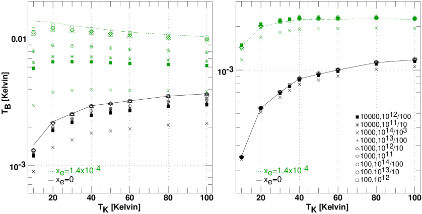
Figure 1: Comparison with LVG calculations for $\mathrm{HCO^{+}}$ J=1-0 at left and J=2-1 at right. Black (solid) and green (dash-dot) lines show calculations using the bulk excitation framework discussed in Section 2 with n(H) = $100~{}{\rm cm}^{-3}$ and dN($\mathrm{HCO^{+}}$)/dv = $10^{12}~{}{\rm cm}^{-2}$ (km s^-1)^-1, for gases with a molecular hydrogen fraction of unity (n($\mathrm{{\rm H}_{2}}$) = n(H)/2) and electron fractions x_e = n(e)/n(H) = 0 and $1.4\times 10^{-4}$ respectively. LVG calculations of the brightness were performed at each value of x_e with parameter combinations n(H), N($\mathrm{HCO^{+}}$) indicated at the lower right in the right-hand panel and with symbols as indicated there. Each n(H), N($\mathrm{HCO^{+}}$) parameter combination is represented by a black and a green symbol. Results of the LVG calculations were scaled by $10^{14}$/(n(H)dN($\mathrm{HCO^{+}}$)/dv) to test the linear dependence that is expected in the limit of weak excitation. For example, the brightnesses of the LVG calculations with n(H) $=10^{4}~{}{\rm cm}^{-3}$, dN($\mathrm{HCO^{+}}$)/dv $=10^{12}~{}{\rm cm}^{-2}$ represented by the solid rectangles were divided by a factor 100 as indicated in the figure legends.

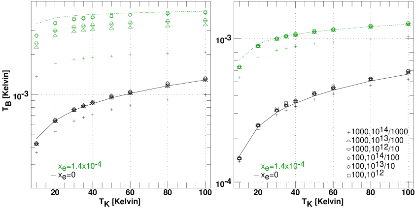
Figure 2: As in Figure 1, but for CS.

2 Weakly-excited lines

2.1 Basic concepts

The approach taken here is a perturbation approximation where the equilibrium condition throughout the molecular rotational energy ladder is pure radiative equilibrium with the cosmic microwave background (CMB) at 2.725 K, minutely disturbed by collisions with ambient particles at the local kinetic temperature $T_{K}$.

Consider the canonical two-level atom with a transition at frequency $\nu$, immersed in a gas of total density of H-nuclei n(H) and kinetic temperature $T_{K}$. The lower and upper levels are labelled l and u, respectively, at energies E_l and E_u above the ground level, having statistical weights g_l and g_u. The number densties of molecules in the lower and upper levels are n_l and n_u and the levels are connected by collisions having rate coefficients $\gamma_{lu}$ and $\gamma_{ul}$ (units of cm${}^{3}~{}\mbox{~{}s${}^{-1}$}$) where $\gamma_{ul}/\gamma_{lu}$ = g_l/g${}_{u}\exp(h\nu/k\mbox{$T_{K}$})$. The upward and downward collision rates (units of  s^-1) are C_lu = n(H)$\gamma_{lu}$ and C_ul = n(H)$\gamma_{ul}$; the rate coefficients $\gamma$ are normalized to reflect this definition as discussed below.

The levels are also connected by the spontaneous emission rate of the upper level, A_ul, and by transitions induced by the cosmic microwave background at temperature T_cmb =2.725 K. The exact solution for the level populations, including the radiation field of the cosmic microwave background is

$$n_{u}/n_{l}=(g_{u}/g_{l})\frac{[p_{\nu}(T_{cmb})+\exp(-h\nu/k\mbox{$T_{K}$})C_{ul}/A_{ul}]}{[p_{\nu}(T_{cmb})+1+C_{ul}/A_{ul}]}$$

where $p_{\nu}(x)=1/(\exp(h\nu/kx)-1)$ and $1+p_{\nu}(x)=1/(1-\exp(-h\nu/kx))$ .

For low-lying rotation transitions in the 3mm band, h$\nu$/k = 4.3 K ($\nu$/100 GHz) and g_l/g${}_{u}<1$, so, at typical kinetic temperatures $>$ 4 K it follows that $\gamma_{ul}<\gamma_{lu}$ and ${\rm C}_{ul}<{\rm C}_{lu}$: If collisional excitation is weak, C${}_{lu}<<$ A_ul, collisional de-excitation is even weaker. Thus in the limit of weak excitation, for the transitions considered here with relatively small values of $h\nu/k$, we will also have $C_{ul}<C_{lu}<<A_{ul}$ and the excess population in the level $u$ over that which would obtain in radiative equilibrium with the cosmic microwave background is

$$\Delta n_{u}=\frac{n_{l}(C_{lu}/A_{ul})}{1+p_{\nu}(T_{cmb})}.$$

This is obtained by differencing Eq. 1 evaluated with and without collisions and neglecting the collisional term in the denominator: note the change from ${\rm C}_{ul}$ in Eq. 1 to ${\rm C}_{lu}$ in Eq. 2 and succeeding equations. Since $\Delta n_{l}=-\Delta n_{u}$, the fractional shift of population out of the lower level, away from the radiative equilibrium established by the cosmic background, $|\Delta n_{l}/n_{l}|=(C_{lu}/A_{ul})/(1+p_{\nu}(T_{cmb}))$, is very small.

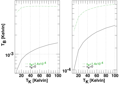
Figure 3: Excitation curves for n(H)$=100~{}{\rm cm}^{-3}$, dN(HNC)/dv $=10^{12}~{}{\rm cm}^{-2}$(km s^-1)^-1 as in Figures 1 and 2, for HNC J=1-0 (left) and J=2-1.

The collision-induced volume emissivity of the line $\epsilon_{u}$ (erg $~{}{\rm cm}^{-3}$ s^-1 sr^-1) is

$$\epsilon_{u}=\Delta n_{u}(h\nu/4\pi)A_{ul}=\frac{(h\nu/4\pi)n_{l}C_{lu}}{1+p_{\nu}(T_{cmb})}$$

independent of A_ul. This is the origin of the approach taken here: in the limit of weak collisional excitation (WCE), spectral lines are merely conduits for the energy that is deposited into them and the energy is radiated at the same rate that it is injected, not at rates determined by the A-coefficients. Independence from the spontaneous emission coefficient that is the main determinant of the critical density has clear implications for the limiting spatial extent of lines of different chemical species.

The simultaneous balancing of the cosmic bacground radiation provides a slight drag on the efficiency of the collisional energy transfer into the line, ie 1+$p_{\nu}(T_{cmb})=1.26$ at 90 GHz.

2.2 Summing to a total rate and column density

In the linear molecules considered here, all upward transitions out of lower-lying levels J $<$ J_u inject energy into the $J_{u}$ - $J_{l}$ line. Thus for the 1-0 line, all rates $C_{0,J^{\prime}}$ for the 0-1, 0-2, etc. transitions are summed; for the J=2-1 line, rates for the transitions 0-2, 0-3 … 0-n and 1-2, 1-3 … 1-n.

Specifically, we define an excitation rate into the level $J_{u}$ as

$$C_{u}=\Sigma_{j<j_{u}}\Sigma_{j^{\prime}\geq j_{u}}f_{j}C_{j,j^{\prime}}/(1+p_{\nu}(T_{cmb})),$$

where the CMB correction is included on a term-by-term basis as a modification of the collision rates $C_{J,J^{\prime}}$ and C_u is normalized so that the effective excitation rate coefficient into the level u, $\gamma_{u}$, is given by

$$C_{u}=n(H)\gamma_{u}.$$

The fraction of molecules in the $l$-th level is calculated in equilibrium with the cosmic microwave background

$$f_{l}=g_{l}\exp(-E_{l}/kT_{cmb})/Q(T_{cmb})$$

and the partition function Q(T_cmb) is calculated as

$$Q(T_{cmb})=\Sigma_{l}g_{l}\exp(-E_{l}/kT_{cmb})$$

with $T_{cmb}$ = 2.725 K. The total number density of molecules summed over all levels is just $n_{l}/f_{l}$. Some 60% of the total rotational population is in the J=0 level for $\mathrm{HCO^{+}}$ and HNC in radiative equilibrium with the CMB, or 40% for CS. The only temperature that appears explicitly in these equations is that of the cosmic background, and the kinetic temperature dependence is entirely contained in the rate coefficients $\gamma_{u}$.

Finally, we define a density n(H)_max for the level u as a fraction q (q $<<1$) of the density at which the total excitation rate into the level u equals its spontaneous emission rate,

$$n(H)_{max}\equiv qA_{ul}/\gamma_{u},$$

independent of the optical depth. Limiting the density in this way is necessary to justify the approximations leading to Eq. 3, but the importance of the requirement that n(H) $\leq$ n(H)_max should not be understood merely as a limit on the excitation temperature: It is also necessary to allow energy injected into the line by collisions to escape the medium without being re-absorbed back into the thermal reservoir of the gas by collisional de-excitation. The weak collisional excitation (WCE) approximation with a fixed proportionality between line brightness and the emission measure only applies when n(H) $\leq$ n(H)_max. This is discussed in more detail in Section 3 where a value q = 1/8 is derived by considering the relationship of the line brightness and the emission measure in the limits of high density and implicit optical depth. When n(H) $>$ n(H)_max there may still be a regime where for suitably faint lines the brightness is linearly proportional to column density (Figure 3 of Linke et al. (1977)), but the ratio of brightness to emission measure decreases because progressively fewer excitations directly result in observable photons.

Our n(H)_max is different from the usual critical density because it is defined in terms of upward rates and because it sums over collisions that do not directly involve the level in question (for instance $\gamma_{1}$ includes 0-1, 0-2, 0-3, etc collisions). The values of A${}_{ul}/\gamma_{u}$ are quite similar to the optically-thin critical densities discussed by Shirley (2015) but our n(H)_max are smaller by the factor q. Values of n(H)_max are given in Tables 2 and 3 for the case q = 1/8 that is discussed in Section 3. For excitation by neutral particles (Table 2), n(H)_max = $5-10\times 10^{3}~{}{\rm cm}^{-3}$ for the J=1-0 lines of $\mathrm{HCO^{+}}$and HNC, and about 10 times higher for their J=2-1 transitions. Values of n(H)_max for CS are about 5 times smaller for both lines. When electron excitation dominates for x${}_{e}=1.4\times 10^{-4}$ (Table 3) the limiting densities n(H)${}_{m}ax$ are on the whole lower by a factor of order 10.

Importantly, note in Tables 2 and 3 that Einstein A-coefficients increase much more rapidly with J_u than do the collision rates and the limiting densities n(H)_max increase with J_u, quite rapidly at the bottom of the rotation ladder. Thus if the weak-excitation case applies to any transition, it is even more valid for yet higher-lying lines.

2.3 Observable line brightness

The total specific energy flux W_u (erg cm${}^{-2}~{}\mbox{~{}s${}^{-1}$}$ sr^-1) from a bulk medium is the line of sight integral of the emissivity $\epsilon_{u}$ , ie

$$W_{u}=\int\epsilon_{u}dL=(h\nu/4\pi)\int n(H)\gamma_{u}n(Y)dL$$

where $\gamma_{u}$ is kept inside the integral to account for variations in the kinetic temperature: The integral is defined and discussed here as the molecular emission measure. The radiative transfer of reabsorption by intervening material along the line of sight is ignored here with the understanding that the range of validity of such an assumption will be derived. The physical basis for the assumption is the limitation to densities below n(H)_max so that scattered photons are not re-absorbed back into the bath of thermal energy by downward collisions.

If the relative abundance of species Y, X(Y) = n(Y)/n(H) is constant, the emitted energy W${}_{u}\propto$ X(Y) $\int n(H)^{2}$ dL is heavily weighted to regions of higher density and strongly influenced by clumping. If the density n(H) and relative abundance X(Y) are constant, W $\propto$ n(H) N(Y) where N(Y) is the total column density of species Y (this is the analog of the LVG calculation described in Section 3). For any density n(H) $\leq$ n(H)_max there is a column density N(Y) that will produce a given output W. The observability of a line is determined by the molecular emission measure, essentially the product of the density and column density.

In terms of observables, the integrated line brightness temperature $T_{B}$ above the black-body background is determined by

$$\int 2k\mbox{$T_{B}$}/\lambda^{2}d\nu=W_{u}$$

or, in velocity units (km s^-1) using Eq. 9

$$\int\mbox{$T_{B}$}d{\rm v}=(\lambda^{2}/8\times 10^{5}\pi)(hc/k)\int n(H)\gamma_{u}n(Y)dL$$

2.4 Actual calculation of the collision rate

The rate coefficients $\gamma_{u}$ are comprised of weighted contributions from collisions with helium, molecular hydrogen and electrons, ie

$$\gamma_{u}=0.0875\gamma_{u}({\rm He})+x_{e}\gamma_{u}(e)+(\mbox{f${}_{\mathrm{{\rm H}_{2}}}$}/2)\gamma_{u}(\mathrm{{\rm H}_{2}})$$

with n(He)/n(H) = 0.0875 (Balser, 2006), x_e = n(e)/n(H) and f${}_{\mathrm{{\rm H}_{2}}}$ = 2n($\mathrm{{\rm H}_{2}}$)/n(H) (maintaining the usual definition of the latter). For the cases where all the hydrogen is in $\mathrm{{\rm H}_{2}}$, n($\mathrm{{\rm H}_{2}}$) = n(H)/2. We ignore collisions with atomic hydrogen that is generally ineffective at exciting molecules (and consider gas in which all the hydrogen is molecular) but include collisions with electrons having a proportion x_e = n(e)/n(H). With the exception of CO to which the WCE limit does not apply over an interesting range of n(H) and/or N(CO) (see Section 4.1), collisions with electrons will usually dominate the excitation when CO does not bear the majority of the gas phase carbon, see Liszt (2012). References to the collision rate coefficients used here are given in Table 1 and the dominance of electron excitation is apparent when collision rates are tabulated (see Appendix A).

2.4.1 Excitation by electrons

For strongly-polar species having permanent dipole moments $\mu>0.5$ Debye, excitation by electrons has a strongly dipole character ($\Delta J=+1$) and rate constants are well represented in separate closed forms for molecular ions (Dickinson & Flower, 1981; Bhattacharyya et al., 1981; Neufeld & Dalgarno, 1989) and neutrals (Dickinson et al., 1977). However, more accurate rates for e-$\mathrm{HCO^{+}}$ and e-HNC collisions have been calculated by Faure et al. (2007a) and Faure et al. (2007b), respectively and for CS by Varambhia et al. (2010). These have the additional virtue that they include the smaller terms with $|\Delta J|>1$ that are important for determining line brightness ratios over the rotation ladder in a single species.

Table 1: References to collision rate coefficients

Species	$\mathrm{{\rm H}_{2}}$	He	electrons
$\mathrm{HCO^{+}}$	Flower (1999)1	scaled $\mathrm{{\rm H}_{2}}$2	Faure et al. (2007a)
HNC	Dumouchel et al. (2011)	Dumouchel et al. (2010)	Faure et al. (2007b)
CS	scaled He	Lique et al. (2006)	Varambhia et al. (2010)
1 See also Yazidi et al. (2014)
2 See also Buffa et al. (2009)

2.4.2 Excitation by helium

Recent calculations for He-molecule collisions are available for HNC and CS, as noted in Table 1. For $\mathrm{HCO^{+}}$ there is a recent reference by Buffa et al. (2009) but the appendix containing the tables of rate coefficients is missing in the article online so we used the $\mathrm{{\rm H}_{2}}$-$\mathrm{HCO^{+}}$ rates scaled downward by a factor 1.4, which is the inverse of the common practice when collisions with He must be substituted for those with $\mathrm{{\rm H}_{2}}$. Examination of the few rates that were tabulated by Buffa et al. (2009) for comparison with earlier results showed that the error introduced by scaling the $\mathrm{{\rm H}_{2}}$ rates will be very small, especially given the He abundance.

2.4.3 Excitation by molecular hydrogen

These are noted in Table 1. For HNC both ortho (odd-J) and para $\mathrm{{\rm H}_{2}}$ collision rates are considered separately and equilibrium between the ortho and para $\mathrm{{\rm H}_{2}}$ populations at the kinetic temperature was assumed: this is very likely to be correct for the case that the electron fraction is appreciable, due to the population of protons. For $\mathrm{HCO^{+}}$ we used the para-$\mathrm{{\rm H}_{2}}$ rates of Flower (1999) as in Liszt (2012): a more recent calculation (Yazidi et al., 2014) differs typically by 10% or less. For CS, unfortunately, the only recent collision rate calculations with neutral particles are those for helium (Lique et al., 2006) but these are also used in RADEX (with appropriate upward scaling by a factor 1.4) so there is at least a basis for comparison.

2.5 Overall behaviour

The individual terms contributing to $\gamma_{1}$ are shown in the Tables in Appendix A for $\mathrm{HCO^{+}}$, HNC and CS excited by He and $\mathrm{{\rm H}_{2}}$ with and without electrons. For excitation by neutral particles, J=0-1 transitions dominate the excitation into the J=1 level at low temperature but only one half - one-third of the total rate is due to direct excitations from the ground state at/above 20 K. This is the origin of the temperature dependence of the line brightnesses shown in Figures 1-3. For a gas with x${}_{e}=1.4\times 10^{-4}$, the collision rate constant per hydrogen is 10-20 times larger but there is little temperature dependence of the collision scheme and direct excitations into the upper level of a transition dominate.

2.6 Scaling with the electron and $\mathrm{{\rm H}_{2}}$ fractions

When electron collisions dominate at x${}_{e}=1.4\times 10^{-4}$ the results here can be considered to be independent of f${}_{\mathrm{{\rm H}_{2}}}$ because the density of electrons n(e) = 0.00014 n(H) has been assumed to be equal to the total density of gas-phase carbon. When electron excitation dominates (see Tables 5 and 6) the implied total density n(H) can be scaled to other electron fractions x_e by keeping the electron density n(e) = x_en(H) constant.

For simplicity the calculations here present only the case f${}_{\mathrm{{\rm H}_{2}}}$ = 1 and ignore collisional excitation by atomic hydrogen, which is generally not considered to be important enough to merit calculation of the excitation rate. Note that the very high rates for excitation of CO by atomic hydrogen calculated by Balakrishnan et al. (2002) and discussed by Liszt (2006) were subsequently refuted by Shepler et al. (2007) and Yang et al. (2013).

When $\mathrm{{\rm H}_{2}}$ excitation dominates, an approximate scaling may be derived by accounting for the fact that n($\mathrm{{\rm H}_{2}}$) = n(H)f${}_{\mathrm{{\rm H}_{2}}}$/2 and that the rate constants for helium are generally considered to be smaller than those for $\mathrm{{\rm H}_{2}}$ by a factor 1.4 following the usual scaling by the thermal speed. This implies a scaling with f${}_{\mathrm{{\rm H}_{2}}}$ such that n(H)(0.125+f${}_{\mathrm{{\rm H}_{2}}}$)/1.125 $\approx$ constant.

3 Validation

The physics discussed here is unexceptionable but as a check on the results and to ascertain the limits of validity of the formalism in opaque media we compare with the results of LVG calculations (Goldreich & Kwan, 1974). An LVG calculation amounts to an evaluation of Eq. 11 at constant density and temperature. Comparison with this widely-used approximation to the radiative transfer problem provides a check on the normalization of the brightness and the effects of radiative trapping which to some degree circumscribe the range over which the excitation can be considered to be weak and the medium may be regarded as being transparent.

In the LVG approximation described by Goldreich & Kwan (1974), the Einstein spontaneous emission coefficients A_ul are replaced by A${}_{ul}\beta_{lu}$ where $\beta_{lu}=(1-\exp(-\tau_{lu}))/\tau_{lu}$ is the photon escape probability derived by Castor (1970) and $\tau_{lu}$ is the line optical depth. In the limit of high optical depth, $\beta_{lu}\rightarrow 1/\tau_{lu}$ and A${}_{ul}\beta_{lu}\rightarrow A_{ul}/\tau_{ul}$, and to account for cases of high optical depth we rewrite Eq. 8 as

$$C_{u}\tau_{lu}/A_{ul}=n(H)\gamma_{u}\tau_{lu}/A_{ul}\leq q.$$

However, $\tau_{lu}/A_{ul}$ is independent of A_ul and after expressing $\tau_{lu}$ in terms of dN(Y)/dv and A_ul etc. using standard formulae relating column density and optical depth (Spitzer, 1978) we can recast Eq. 13 as a limit on the density-column density product,

$$n(H)\frac{dN(Y)}{d{\rm V}}\leq q\frac{8\times 10^{5}\pi Q(T_{cmb})\exp(E_{l}/kT_{cmb})}{g_{u}\lambda^{3}\gamma_{u}}$$

with velocity expressed in km s^-1. There is only a slow temperature dependence over the range 10 - 80 K and limiting values for $T_{K}$ = 30 K are shown in Table 4 for q = 1/8 with $x_{e}=0$ and $x_{e}=1.4\times 10^{-4}$.

We chose q = 1/8 after running many models because it limits the divergence from the LVG calculations to 20% or less when n(H) $\lesssim$ n(H)_max. For the species discussed here, using q = 1/8 to limit the upward rate C_u is equivalent to C₁₀/A${}_{10}\lesssim 1/20$ at 10 K or C₁₀/A${}_{10}\lesssim 1/50$ at/above 30 K which certainly justifies the approximations that were assumed to derive the basic equations.

Using Eq. 11, Eq. 14 can be rewritten as an upper limit on the observed line brightness in remarkably compact form, namely

$$T_{B}\leq q\frac{h\nu}{k}\frac{Q(T_{cmb})\exp(E_{l}/kT_{cmb})}{g_{u}},$$

showing that the applicability of the WCE approximation can be understood solely in terms of the line brightness, independent of the means of excitation or the underlying physical conditions, given only that n(H) $\leq$ n(H)_max. A similar conclusion can be found in the text of Linke et al. (1977) following their Equation 15, but without the explicit caveat on the density. Values of the limiting brightness temperature are given in Table 4. These are 0.3 K for the J=1-0 lines and 0.8 - 1.7 K for J=2-1.

3.1 Computational results

Figures 1 and 2 show direct comparisons between the bulk excitation results and those of full LVG calculations, for $\mathrm{HCO^{+}}$ and CS respectively, with the J=1-0 lines at left and J=2-1 at right in each case. Results are shown for x${}_{e}=0$ in black (these lay lower) and for $x_{e}=1.4\times 10^{-4}$ in green. Eq. 12 was evaluated at n(H) $=100~{}{\rm cm}^{-3}$ and molecular column densities dN(mol)/dv $=10^{12}~{}{\rm cm}^{-2}(\mbox{km\,s${}^{-1}$})^{-1}$, ie. n(H)dN(mol)/dv $=10^{14}$cm${}^{-5}(\mbox{km\,s${}^{-1}$})^{-1}$. The LVG calculations were carried out at various density, column density products as shown in the panels of the figures and their results were normalized to a product of $10^{14}{\rm cm}^{-5}(\mbox{km\,s${}^{-1}$})^{-1}$: for instance, the LVG brightnesses computed for n(H) = $10^{3}~{}{\rm cm}^{-3}$, dN(mol)/dv $=10^{13}~{}{\rm cm}^{-2}(\mbox{km\,s${}^{-1}$})^{-1}$ were divided by 100. The actual line brightnesses represented in the panels vary by factors up to almost $10^{3}$ and the optical depths range up to almost 100 for the J=1-0 line of $\mathrm{HCO^{+}}$ while retaining a high degree of linear proportionality to the density-column density product within the weak-excitation regime as described in the previous Section.

Table 2: Limiting density n(H)_max for q = 1/8 and $x_{e}=0$

Species	$J_{u}-J_{l}$	5 K	10 K	20 K	30 K	40 K	60 K	80 K
					$~{}{\rm cm}^{-3}$
$\mathrm{HCO^{+}}$	1-0	1.79E+04	1.39E+04	9.01E+03	7.77E+03	6.72E+03	6.13E+03	5.63E+03
	2-1	3.40E+05	1.89E+05	8.77E+04	6.83E+04	5.49E+04	4.77E+04	4.23E+04
HNC	1-0	4.00E+04	2.22E+04	1.51E+04	1.27E+04	1.14E+04	9.71E+03	8.76E+03
	2-1	8.93E+05	2.94E+05	1.58E+05	1.25E+05	1.08E+05	8.89E+04	7.84E+04
CS	1-0	1.22E+04	3.64E+03	2.66E+03	2.23E+03	1.99E+03	1.66E+03	1.46E+03
	2-1	1.06E+05	2.45E+04	1.53E+04	1.21E+04	1.05E+04	8.48E+03	7.33E+03

Table 3: Limiting density n(H)_max for q = 1/8 and $x_{e}=1.4\times 10^{-4}$

Species	$J_{u}-J_{l}$	5 K	10 K	20 K	30 K	40 K	60 K	80 K
				$~{}{\rm cm}^{-3}$
$\mathrm{HCO^{+}}$	1-0	1.68E+03	1.43E+03	1.45E+03	1.55E+03	1.61E+03	1.74E+03	1.83E+03
	2-1	6.17E+04	3.27E+04	2.39E+04	2.23E+04	2.12E+04	2.12E+04	2.10E+04
HNC	1-0	3.96E+03	2.70E+03	2.28E+03	2.19E+03	2.17E+03	2.15E+03	2.16E+03
	2-1	2.07E+05	8.64E+04	5.55E+04	4.79E+04	4.43E+04	4.04E+04	3.82E+04
CS	1-0	6.64E+02	4.99E+02	4.50E+02	4.34E+02	4.25E+02	4.15E+02	4.08E+02
	2-1	9.48E+03	5.22E+03	4.04E+03	3.66E+03	3.46E+03	3.21E+03	3.06E+03

3.1.1 $\mathrm{HCO^{+}}$

Figure 1 shows computational results for the J=1-0 and J=2-1 lines of $\mathrm{HCO^{+}}$ at left and right, respectively. The two lines have optical depth of unity at dN($\mathrm{HCO^{+}}$)/dv = 1.1 and 2.2 $\times 10^{12}~{}{\rm cm}^{-2}$ (km s^-1)^-1, respectively.

Without electrons, the entries in Table 4 predict that the bulk excitation and LVG calculations should diverge for n(H)dN($\mathrm{HCO^{+}}$)/dv $\gtrsim 2\times 10^{16}$cm${}^{-5}(\mbox{km\,s${}^{-1}$})^{-1}$ at low density and this is manifested in the calculations: with n(H) $=10^{3}~{}{\rm cm}^{-3}$, the deviation from the LVG calculation increases from 7% at dN($\mathrm{HCO^{+}}$)/dv = $10^{13}~{}{\rm cm}^{-2}(\mbox{km\,s${}^{-1}$})^{-1}$ where $T_{B}$ $\lesssim$ 0.33K to 40% at dN($\mathrm{HCO^{+}}$)/dv = $10^{14}~{}{\rm cm}^{-2}(\mbox{km\,s${}^{-1}$})^{-1}$ where $T_{B}$ $\lesssim$ 2K. The density criterion is more important than a limit on the optical depth: the deviation is larger for n(H)$=10^{4}~{}{\rm cm}^{-3}$, dN($\mathrm{HCO^{+}}$)/dv $=10^{12}~{}{\rm cm}^{-2}(\mbox{km\,s${}^{-1}$})^{-1}$, where the optical depth is 0.9, than for n(H) $=10^{2}~{}{\rm cm}^{-2}$, dN($\mathrm{HCO^{+}}$)/dv $=10^{14}~{}{\rm cm}^{-2}~{}(\mbox{km\,s${}^{-1}$})^{-1}$ where it is 90. The calculations also demonstrate the dependence on the density-column density product, ie the results coincide for n(H) $=10^{2}~{}{\rm cm}^{-3}$, dN($\mathrm{HCO^{+}}$)/dv $=10^{14}~{}{\rm cm}^{-2}~{}(\mbox{km\,s${}^{-1}$})^{-1}$ and for n(H) $=10^{3}~{}{\rm cm}^{-3}$, dN($\mathrm{HCO^{+}}$)/dv $=10^{13}~{}{\rm cm}^{-2}$ (km s^-1)^-1.

Also as predicted, the range of validity is more limited in terms of both density and the density-column density product when electrons dominate the excitation while observing the same limit on the brightness. The ranges of brightness and n(H)dN(mol)/dv over which the bulk excitation and LVG results coincide are much wider for the J=2-1 line than for J=1-0.

3.1.2 CS

Figure 2 shows computational results for the J=1-0 and J=2-1 lines of CS at left and right, respectively. The two lines have optical depth of unity at dN(CS)/dv = 9.8 and 8.2 $\times 10^{12}~{}{\rm cm}^{-2}$ (km s^-1)^-1, respectively.

CS ostensibly differs from $\mathrm{HCO^{+}}$ in several notable ways even if the brightness temperature limits in Table 4 are comparable: The CS J=1-0 transition lies much lower (49 GHz) where the CMB correction is 2 times larger and the lines require 4-8 times higher column density to achieve unit optical depth. Cross-sections for excitation by neutral particles are much smaller because CS is physically more compact (Tables 5 and 6). The limiting densities in Table 2 are 2-3 times lower for CS than for $\mathrm{HCO^{+}}$ but the limiting density-column density products are larger by the same factor and CS requires about an order of magnitude higher column density to emit the same amount of energy in the J=1-0 line, compared to $\mathrm{HCO^{+}}$. In the end much of this is compensated in the conversion to brightness temperature and (like HNC) the J=1-0 lines of CS are 3-4 times weaker than $\mathrm{HCO^{+}}$ for a given density-column density product.

As for $\mathrm{HCO^{+}}$, the LVG and bulk-excitation calculations diverge when the density-column density product or brightness exceed the limiting values shown in Table 4.

3.1.3 HNC

Figure 3 shows computational results for the J=1-0 and J=2-1 lines of HNC at left and right, respectively. The two lines have optical depth of unity at dN(HNC)/dv = 1.8 and 3.7 $\times 10^{12}~{}{\rm cm}^{-2}$ (km s^-1)^-1 respectively. The parameters for HNC are similar to those for $\mathrm{HCO^{+}}$ and results are shown without comparison with LVG results.

Table 4: Limiting brightness temperature and n(H) dN(mol)/dv¹ for q = 1/8

Species	$J_{u}-J_{l}$	$T_{B}$	n(H)dN(mol)/dv (x${}_{e}=0)$	n(H)dN(mol)/dv (x${}_{e}=1.4\times 10^{-4})$
		Kelvins	cm-5(km s-1)-1	cm-5(km s-1)-1
$\mathrm{HCO^{+}}$	1-0	0.30	1.9E16	1.9E15
	2-1	1.72	4.4E17	6.2E16
HNC	1-0	0.30	4.1E16	3.6E15
	2-1	1.77	1.0E18	1.5E17
CS	1-0	0.26	4.4E16	3.0E15
	2-1	0.75	4.6E17	4.4E16

¹ Evaluated at $T_{K}$ = 30 K

3.2 Using bulk excitation to replace or scale LVG calculations

Despite the elaborate nature of the preceding disussion, using the calculations illustrated in Figures 1 - 3 is straightforward. Given a brightness that obeys the limits in Table 4, or an integrated brightness whose peak brightness obeys the limit, divide by the value in the appropriate curve, multiply by $10^{14}$ and that is n(H)dN(Y)/dv or n(H)N(Y) at the assumed temperature and electron fraction. Dependencies on the assumed parameters are clearly manifest in ways that are not always apparent from interpreting the numerical results of large grids of LVG model calcuations. Conversely, knowing a priori how LVG results will scale, a single LVG calculation can replace a grid of numerical solutions.

As an example, consider the observations of $\mathrm{HCO^{+}}$ J=1-0 lines in absorption in diffuse and translucent clouds with measured N($\mathrm{HCO^{+}}$) $\approx 10^{12}~{}{\rm cm}^{-2}$ accompanied by weak emission with integrated brightnesses $\lesssim 0.03$ K-km s^-1 (Lucas & Liszt, 1996). At $T_{K}$ = 30 K with x${}_{e}=1.4\times 10^{-4}$ the implied density-column density product from Figure 1 is n(H)N($\mathrm{HCO^{+}}$) $=2.2\times 10^{14}~{}{\rm cm}^{-5}$, implying n(H) $\approx 220~{}{\rm cm}^{-3}$. Without electrons the derived density ranges from ten times higher at $T_{K}$ = 10 K to three times at $T_{K}$ = 80K.

Alternatively, consider the weak but ubiquitous emission from strongly-polar species that accompanies carbon monoxide emission in surveys of the inner Galactic plane with brightness about 2% that of $\mathrm{{}^{12}CO}$ (Liszt, 1995; Helfer & Blitz, 1997). The widespread nature of this emission was somewhat surprising given the conventional wisdom about the difficulties of exciting it, but a variety of considerations led to the conclusion that it was arising in gas of rather moderate density. At 1%-2% the brightness of CO, the observed brightnesses of $\mathrm{HCO^{+}}$, HCN, CS, etc overwhelmingly lie within the range of applicability of our discussion. A reanalysis of these observations using recent values for the molecular abundances and excitation rates should lead to an improved understanding of the structure of inner-Galaxy molecular clouds.

4 Other considerations

4.1 Extension to other species

The calculation described here works well for molecules that have low-lying transitions in the mm-wave regime where an explicit limit on the upward collision rates for low-lying levels also suitably limits the downward rates, guaranteeing weak collisional excitation while allowing the free escape of energy in the lines. Moreover, most commonly-observed molecules have permanent dipole moments of about 1 Debye or more, making the spontaneous emission rates high enough to allow consideration of an interesting range of parameter space. However many commonly-observed molecules are non-linear and/or have strongly-resolved hyperfine structure, complications that make calculation of the collisional rate coefficients more difficult and limit our interpretative abilities.

The calculation described here has only a very limited range of validity for CO whose small dipole moment (0.11 Debye) leads to A${}_{10}\approx 7\times 10^{-8}$ s^-1, some 600 times smaller than for $\mathrm{HCO^{+}}$, and it is not interesting. Even far below the levels of detectability, CO is already in a regime where the brightness of its J=1-0 transition is proportional to column density and largely independent of density (Liszt, 2007). Somewhat like C I, the excitation temperature of the J=1-0 line of CO is sensitive to the thermal pressure of $\mathrm{{\rm H}_{2}}$, not the $\mathrm{{\rm H}_{2}}$ density alone, when CO is strongly sub-thermally excited (Liszt & Pety, 2012).

The calculation described here is also valid over an interesting range of parameter space for CH whose J=1-0 transition lies much higher near 530 GHz, but CH can also be treated well as a two-level atom under most circumstances in which it would be expected to have substantial abundances. Perhaps a more interesting case would be CH⁺ that is produced and observed in shocked regions at higher temperature (Godard et al., 2012).

4.2 Distinguishing density and abundance variations

The range of possible behaviour embodied in Eq. 9 and 11 for the line of sight integral is richer and more complex than the case of constant density and temperature used in the comparison with LVG calculations in the previous Section. However, to the extent that different species observed over the same cloud sample more or less the same material and are subject to the same run of density n(H) at any position, their limiting brightness distributions will mainly reflect their abundances: If one species is more spatially confined than another, that is because of its chemistry – the spatial distribution of its abundance and column density – not because it is more poorly excited. When the ratio of brightnesses of two species changes from position to position that mainly reflects variation in their relative abundances.

In the weak excitation limit, the ratio of brightnesses of two lines of the same molecule given by Eq. 9 is nominally independent of the density, or even the variation of density along the line of sight, in even the (supposedly) most density-sensitive species. If the ratio changes from position to position, the change can only arise from variations in the temperature or ionization fraction in the host gas. For excitation by neutral particles, the brightness of the 1-0 line of $\mathrm{HCO^{+}}$ at left in Figure 1 increases by 50% when going from 10 to 20 K while the brightness of the 2-1 line doubles. There is relatively little temperature variation for the J=1-0 lines when excited by electrons, but rather more variation for the J=2-1 line of HNC.

5 Summary

In Section 2 we re-derived expressions for the emergent brightness of mm-wave molecular rotational transitions in the limit where the overall collisional excitation rates are small compared to the spontaneous emission rates, as defined by a suitably-defined maximum density n(H)_max. The emergent brightnesses of the lines of a species Y can be expressed as an emission measure - the line of sight integral of the product of two number densities n(H) $\times$ n(Y) - with a constant of proportionality that depends on fundamental constants and an appropriately-defined kinetic temperature-dependent excitation rate coefficient. The excitation rate coefficient is found by summing over the rate constants for individual upward transitions without solving the multi-level rate equations for the simultaneous equilibrium of all the individual states.

In this limit, the line brightnesses can be calculated without mention of the rotational excitation temperatures, optical depths, spontaneous emission rates or critical densities etc. that are usually cited as being important for the excitation and detectability of weak lines. This is a direct consequence of the fact that thermal energy injected into the molecular energy ladder by upward collisions emerges from the gas without being reabsorbed into the thermal energy reservoir by collisional de-excitation, even after repeated scatterings. The only condition necessary for the detectability of a line is that the carrier molecule can channel enough of the ambient thermal energy into the line.

In Section 3 we evaluated the formalism for the low-lying transitions of the three commonly-observed molecules $\mathrm{HCO^{+}}$, HNC and CS. To test the extent of the weak collisional excitation limit and the bulk excitation calculation we compared the results of the closed-form expressions for the line brightness with the results of LVG escape probability solutions of the multi-level equilibrium. Using the limiting form for the escape probability $\beta\rightarrow 1/\tau$ at high optical depth, we derived formal limits on the product n(H)dN(Y)/dv that are directly equivalent to limits on the emergent line brightness. The brightness limits are expressed in a simple form that has little reference to the underlying formalism or even the structure of the molecule in question. The closed form and numerical solutions diverge in expected ways, allowing us to set the numerical value of the sole free parameter of the formalism, which defines the numerical meaning of “weak” excitation.

We tabulated parameters for $\mathrm{HCO^{+}}$, HNC and CS by limiting the divergence between the closed form and LVG approximations (both are approximations of different kinds) to 20% of the predicted line brightness in the most extreme case. Limits on the allowable densities n(H)_max in Tables 2 and 3 are perhaps surprisingly high, typically $10^{4}~{}{\rm cm}^{-3}$ for excitation by $\mathrm{{\rm H}_{2}}$ and He in the J=1-0 lines of $\mathrm{HCO^{+}}$, HNC, although 4-5 times smaller for CS. Allowable densities are much larger for higher-lying lines and lower for excitation by electrons when x${}_{e}=1.4\times 10^{-4}$ and the CO fraction in the gas is presumably small. Limits on n(H)dN/dv and the limiting line brightnesses are shown in Table 4. The latter are 0.3 K for J=1-0 lines and 0.8 - 1.8 K for J=2-1. Cases covered by the weak excitation limit may extend to up quite high optical depth at appreciable density, for instance up to optical depth $\tau_{01}=10$ at n(H) $=1000~{}{\rm cm}^{-3}$ or $\tau_{01}=100$ at n(H) $=100~{}{\rm cm}^{-3}$ for the calculations shown in Figure 1.

The full range of behaviour is implicitly contained in the defining equations which relate the integrated brightness of lines of species Y to the line of sight integral of n(H)n(Y) that is the molecular emission measure. When the relative abundance n(Y)/n(H) is constant, the integrated brightness is proportional to the line of sight integral of n(H)² which is susceptible to clumping and dominated by regions of high density. When the density is constant, the integrated line brightness is proportional to n(H)N(Y) and perhaps weighted to regions of higher kinetic temperature where the excitation rate is larger. The typical LVG or escape probability calculation corresponds to the limiting case where everything inside the line of sight integral is constant, so the expressions derived here can, under the proper conditions, replace grids of numerical solutions while making explicit the dependences on the assumed density and temperature etc that are not necessarily exemplified in the numerical work.

Appendix A Excitation of the 1-0 transition

Tables 5 and 6 give Einstein A-coefficients for the upper levels J_u and the upward collision rate terms $f_{0}\gamma_{0,J_{u}}/(1+p_{\nu}(T_{cmb})$ used to compute the excitation of the J=1 level in Eq. 4. Results are given for for x${}_{e}=0$ and x${}_{e}=1.4\times 10^{-4}$. Units are $10^{-10}$ cm³ s^-1.

For excitation by $\mathrm{{\rm H}_{2}}$ (Table 5), direct excitations into the J=1 level dominate for $T_{K}$ $\lesssim 10$ K but at 80 K they comprise only about 1/3 of the total rate. This is the origin of the temperature dependences shown in Figures 1 - 3. For electron excitation (Table 6) direct excitations into the J=1 level dominate at all temperatures and the temperature dependence is weaker, again as shown in Figures 1-3.

Table 5: Einstein A-coefficients A${}_{J_{u},J_{u-1}}$ and upward collision rate terms entering Eq. 4 with x${}_{e}=0$.

				$\mathrm{HCO^{+}}$
$J_{l}-J_{u}$	A${}_{J_{u},J_{u-1}}$	5 K	10 K	20 K	30 K	40 K	60 K	80 K
	s-1				$10^{-10}{\rm cm}^{3}$  s-1
0-1	4.09E-05	1.2886	1.3877	1.4945	1.4630	1.4411	1.3937	1.3610
0-2	3.92E-04	0.3636	0.6125	1.0315	1.1406	1.2249	1.2249	1.2249
0-3	1.42E-03	0.0541	0.1803	0.6010	0.7944	0.9682	1.0443	1.1018
0-4	3.49E-03	0.0030	0.0249	0.2051	0.3606	0.5380	0.6821	0.8071
0-5	6.96E-03	0.0001	0.0020	0.0505	0.1285	0.2492	0.3913	0.5388
0-6	1.22E-02	0.0000	0.0002	0.0145	0.0526	0.1314	0.2536	0.4043
				HNC
$J_{l}-J_{u}$	A${}_{J_{u},J_{u-1}}$	5 K	10 K	20 K	30 K	40 K	60 K	80 K
	s-1				$10^{-10}{\rm cm}^{3}$  s-1
0-1	2.60E-05	0.4009	0.5559	0.6532	0.7036	0.7506	0.8401	0.9050
0-2	2.49E-04	0.0895	0.2999	0.5245	0.6274	0.6793	0.7179	0.7351
0-3	9.02E-04	0.0020	0.0283	0.0978	0.1417	0.1789	0.2617	0.3303
0-4	2.22E-03	0.0000	0.0024	0.0254	0.0557	0.0852	0.1353	0.1678
0-5	4.43E-03	0.0000	0.0002	0.0046	0.0146	0.0266	0.0511	0.0736
0-6	7.77E-03	0.0000	0.0000	0.0005	0.0026	0.0060	0.0151	0.0252
				CS
$J_{l}-J_{u}$	A${}_{J_{u},J_{u-1}}$	5 K	10 K	20 K	30 K	40 K	60 K	80 K
	s-1				$10^{-10}{\rm cm}^{3}$  s-1
0-1	1.69E-06	0.0404	0.1023	0.1028	0.1028	0.1020	0.1017	0.1018
0-2	1.62E-05	0.0221	0.0895	0.1206	0.1354	0.1433	0.1623	0.1813
0-3	5.87E-05	0.0019	0.0154	0.0316	0.0413	0.0474	0.0555	0.0609
0-4	1.44E-04	0.0004	0.0078	0.0266	0.0404	0.0500	0.0630	0.0730
0-5	2.88E-04	0.0000	0.0014	0.0091	0.0173	0.0242	0.0340	0.0404
0-6	5.06E-04	0.0000	0.0003	0.0038	0.0097	0.0158	0.0263	0.0344

Table 6: Einstein A-coefficients A${}_{J_{u},J_{u-1}}$ and upward collision rate terms entering Eq. 4 for x${}_{e}=1.4\times 10^{-4}$.

				$\mathrm{HCO^{+}}$
$J_{l}-J_{u}$	A${}_{J_{u},J_{u-1}}$	5 K	10 K	20 K	30 K	40 K	60 K	80 K
	s-1				$10^{-10}{\rm cm}^{3}$  s-1
0-1	4.09E-05	17.1290	18.9274	16.7029	14.7472	13.3841	11.6152	10.5138
0-2	3.92E-04	0.9935	2.2323	3.2158	3.3514	3.3553	3.1577	2.9868
0-3	1.42E-03	0.0627	0.2607	0.8078	1.0536	1.2462	1.3251	1.3722
0-4	3.49E-03	0.0032	0.0331	0.2550	0.4437	0.6408	0.8016	0.9307
0-5	6.96E-03	0.0001	0.0021	0.0527	0.1338	0.2570	0.4021	0.5511
0-6	1.22E-02	0.0000	0.0002	0.0146	0.0531	0.1323	0.2551	0.4061
				HNC
$J_{l}-J_{u}$	A${}_{J_{u},J_{u-1}}$	5 K	10 K	20 K	30 K	40 K	60 K	80 K
	s-1				$10^{-10}{\rm cm}^{3}$  s-1
0-1	2.60E-05	4.8820	6.9694	7.9674	8.1270	8.1086	7.9518	7.7590
0-2	2.49E-04	0.0895	0.2999	0.5245	0.6274	0.6793	0.7179	0.7351
0-3	9.02E-04	0.0020	0.0283	0.0978	0.1417	0.1789	0.2617	0.3303
0-4	2.22E-03	0.0000	0.0024	0.0254	0.0557	0.0852	0.1353	0.1678
0-5	4.43E-03	0.0000	0.0002	0.0046	0.0146	0.0266	0.0511	0.0736
0-6	7.77E-03	0.0000	0.0000	0.0005	0.0026	0.0060	0.0151	0.0252
				CS
$J_{l}-J_{u}$	A${}_{J_{u},J_{u-1}}$	5 K	10 K	20 K	30 K	40 K	60 K	80 K
	s-1				$10^{-10}{\rm cm}^{3}$  s-1
0-1	1.69E-06	1.1359	1.4180	1.4989	1.5084	1.5015	1.4756	1.4457
0-2	1.62E-05	0.0486	0.1366	0.1771	0.1920	0.1985	0.2137	0.2293
0-3	5.87E-05	0.0021	0.0162	0.0331	0.0429	0.0492	0.0572	0.0626
0-4	1.44E-04	0.0004	0.0078	0.0267	0.0404	0.0501	0.0630	0.0730
0-5	2.88E-04	0.0000	0.0014	0.0091	0.0173	0.0242	0.0340	0.0404
0-6	5.06E-04	0.0000	0.0003	0.0038	0.0097	0.0158	0.0263	0.0344

References

- Balakrishnan et al. (2002) Balakrishnan, N., Yan, M., & Dalgarno, A. 2002, ApJ, 568, 443
- Balser (2006) Balser, D. S. 2006, AJ, 132, 2326
- Bhattacharyya et al. (1981) Bhattacharyya, S. S., Bhattacharyya, B., & Narayan, M. V. 1981, ApJ, 247, 936
- Buffa et al. (2009) Buffa, G., Dore, L., & Meuwly, M. 2009, MNRAS., 397, 1909
- Castor (1970) Castor, J. I. 1970, MNRAS, 149, 111
- Dickinson & Flower (1981) Dickinson, A. S. & Flower, D. R. 1981, MNRAS, 196, 297
- Dickinson et al. (1977) Dickinson, A. S., Phillips, T. G., Goldsmith, P. F., Percival, I. C., & Richards, D. 1977, A&A, 54, 645
- Dubernet et al. (2013) Dubernet, M.-L., Alexander, M. H., Ba, Y. A., et al. 2013, A&A, 553, A50
- Dumouchel et al. (2010) Dumouchel, F., Faure, A., & Lique, F. 2010, MNRAS, 406, 2488
- Dumouchel et al. (2011) Dumouchel, F., Kłos, J., & Lique, F. 2011, Physical Chemistry Chemical Physics (Incorporating Faraday Transactions), 13, 8204
- Faure et al. (2007a) Faure, A., Tennyson, J., Varambhia, H. N., et al. 2007a, in Molecules in Space and Laboratory, ed. J. L. Lemaire, & F. Combes
- Faure et al. (2007b) Faure, A., Varambhia, H. N., Stoecklin, T., & Tennyson, J. 2007b, MNRAS, 382, 840
- Flower (1999) Flower, D. R. 1999, MNRAS, 305, 651
- Godard et al. (2012) Godard, B., Falgarone, E., Gerin, M., et al. A&A, 540, A87
- Goldreich & Kwan (1974) Goldreich, P. & Kwan, J. 1974, ApJ, 189, 441
- Goldsmith et al. (2012) Goldsmith, P. F., Langer, W. D., Pineda, J. L., & Velusamy, T. 2012, Astrophys. J., Suppl. Ser., 203, 13
- Helfer & Blitz (1997) Helfer, T. T. & Blitz, L. 1997, ApJ, 478, 233
- Levrier et al. (2012) Levrier, F., Le Petit, F., Hennebelle, P., et al. 2012, A&A, 544, A22
- Linke et al. (1977) Linke, R. A., Goldsmith, P. F., Wannier, P. G., Wilson, R. W., & Penzias, A. A. 1977, ApJ, 214, 50
- Lique et al. (2006) Lique, F., Spielfiedel, A., & Cernicharo, J. 2006, A&A, 451, 1125
- Liszt (1995) Liszt, H. S. 1995, ApJ, 442, 163
- Liszt (2006) —. 2006, A&A, 458, 507
- Liszt (2007) —. 2007, A&A, 476, 291
- Liszt (2012) —. 2012, A&A, 538, A27
- Liszt & Pety (2012) Liszt, H. S. & Pety, J. 2012, A&A, 541, A58
- Lucas & Liszt (1996) Lucas, R. & Liszt, H. S. 1996, A&A, 307, 237
- Mangum & Shirley (2015) Mangum, J. G. & Shirley, Y. L. 2015, PASP, 127, 266
- Neufeld & Dalgarno (1989) Neufeld, D. A. & Dalgarno, A. 1989, Phys. Rev. A, 40, 633
- Penzias (1975) Penzias, A. A. 1975, in Atomic and Molecular Physics and the Interstellar Matter, ed. R. Balian, P. Encrenaz, & J. Lequeux (Les Houches session 26; Amsterdam: North-Holland), 373–408
- Shepler et al. (2007) Shepler, B. C., Yang, B. H., Dhilip Kumar, T. J., et al. A. 2007, A&A, 475, 15
- Shirley (2015) Shirley, Y. L. 2015, PASP, 127, 299
- Snell et al. (2000) Snell, R. L., Howe, J. E., Ashby, M. L. N., et al. 2000, ApJ, 539, L93
- Spitzer (1978) Spitzer, L. 1978, Physical processes in the interstellar medium (New York Wiley-Interscience, 1978. 333 p.)
- van der Tak et al. (2007) van der Tak, F. F. S., Black, J. H., Schöier, F. L., Jansen, D. J., & van Dishoeck, E. F. 2007, A&A, 468, 627
- Varambhia et al. (2010) Varambhia, H. N., Faure, A., Graupner, K., Field, T. A., & Tennyson, J. 2010, MNRAS, 403, 1409
- Wannier et al. (1991) Wannier, P. G., Pagani, L., Kuiper, T. B. H., et al. 1991, ApJ, 377, 171
- Yang et al. (2013) Yang, B., Stancil, P. C., Balakrishnan, N., Forrey, R. C., & Bowman, J. M. 2013, ApJ, 771, 49
- Yazidi et al. (2014) Yazidi, O., Ben Abdallah, D., & Lique, F. 2014, MNRAS, 441, 664