Ab initio study of the strain dependence of thermopower in electron-doped SrTiO₃

Abstract

In this paper we explore the different mechanisms that affect the thermopower of a band insulating perovskite (in this case, SrTiO₃) when subject to strain (both compressive or tensile). We analyze the high temperature, entropy dominated limit and the lower temperature, energy-transport regime. We observe that the effect of strain in the high-temperature Seebeck coefficient is small at the concentration levels of interest for thermoelectric applications. However, the effective mass changes substantially with strain, which produces an opposite effect to that of the degeneracy-breakups brought about by strain. In particular, we find that the thermopower can be enhanced by applying tensile strain in the adequate regime. We conclude that the detrimental effect of strain in thermopower due to band splitting is a minor effect that will not hamper the optimization of the thermoelectric properties of oxides with t_2g-active bands by applying strain.

I Introduction

Oxides have become an interesting playground to search for new materials with enhanced thermoelectric (TE) properties. They can be easily synthesized, they are chemically stable, they can be nanostructured in the form of films,Ohtomo and Hwang (2004) nanoparticlesLópez-Quintela et al. (2003) and nanowires,Maeng et al. (2008) and they span a huge range of chemical compositions and doping.Mannhart and Schlom (2010) Examples of oxides with promising TE properties are the family of misfit layered cobaltatesLimelette et al. (2005); Terasaki et al. (1997) and also SrTiO₃Moos et al. (1995) and its nanostructures.Ohta et al. (2007)

In standard semiconductors, the parameters entering the TE figure of merit,Snyder and Toberer (2008) namely the electrical conductivity, the Seebeck coefficient and the thermal conductivity (in particular its electronic component) are usually coupled so that improving the electrical conductivity has a negative effect in the Seebeck coefficient and the thermal conductivity, and vice versa. Many different routes have been proposed to optimize the figure of merit.Lu et al. (2016); Zheng et al. (2013) One way to enhance the TE response of a material is, on one hand, to play with the phonon part of the thermal conductivity,Yu et al. (2008); Dresselhaus et al. (2007) and in order to decouple the electronic components, strain has been suggested as a promising mechanism to do so.Li et al. (2010) Oxides, with their flexible d electrons, should be more permeable to changes and tunability of their electronic structure with strainPardo et al. (2013) and nanostructuringChen et al. (2003) than standard sp semiconductors. d electron systems show many different phases as a product of the coupling between lattice, spin, charge and orbital degrees of freedom,Imada et al. (1998) which could help tuning the band structure at will and modify the TE response in the desired direction.

It is hence very important to understand how d-electron bands are affected by strain. In the past, strain has been proposed as a natural way to produce band engineering in oxides.Qiao et al. (2011) In principle, in a cubic system strain has a detrimental effect by reducing orbital degeneracy and hence reducing the thermopower, particularly at high temperatures.Sarantopoulos et al. (2015) To explore quantitatively the effects of strain and its related symmetry breaking in the actual values of the thermopower for typical oxides, we have chosen to model this using a very simple cubic perovskite oxide SrTiO₃, that is naturally n-doped. Those electrons will populate the t_2g bands which will respond to strain in different ways depending on its magnitude, its sign, but more importantly, also depending on the doping level. We will analyze in detail the effects of strain not only in transport properties but also in terms of disturbing the electronic degeneracies in a t_2g electron system and how these affect the thermopower and the effective mass of the system.

In principle, the findings obtained for SrTiO₃ should provide a general platform for understanding similar mechanisms that occur in other perovskite-related oxides of interest for TE applications.Villar Arribi et al. (2016)

II Computational procedures

Ab initio electronic structure calculations based on the density functional theory (DFT)Hohenberg and Kohn (1964); Kohn and Sham (1965) have been performed using an all-electron full potential code (wien2kSchwarz and Blaha (2003)) on SrTiO₃.

The exchange-correlation term is parametrized depending on the case. We have used the generalized gradient approximation (GGA) in the Wu-CohenWu and Cohen (2006) scheme for structural optimizations (volume optimizations). For the electronic structure calculations we have used the semilocal potential developed by Tran and Blaha as a modification of the Becke-Johnson potential.Tran and Blaha (2009) This method typically allows the calculation of band gaps with an accuracy similar to the much more expensive GW or hybrid methods,Koller et al. (2011) and in particular for SrTiO₃ it gives an accurate band gap.Sarantopoulos et al. (2015) However, effective masses are not improved with respect to standard LDA/GGA functionals.Dixit et al. (2012)

The calculations were performed with a converged k-mesh and a value of R_mtK_max= 7.0. Spin-orbit coupling (SOC) was introduced in a second variational manner using the scalar relativistic approximation.Singh and Nordstrom (2006) The $R_{mt}$ values used were in a.u.: 2.50 for Sr, 1.86 for Ti and 1.69 for O when studying SrTiO₃.

Transport properties have been calculated using the BoltzTrapMadsen and Singh (2006) code. This solves Boltzmann transport equation from first-principles calculations within the constant scattering time approximation. This strategy will allow us to obtain the Seebeck coefficient at different temperatures, which is, within that approximation, independent of the scattering time. These calculations require an even finer k-mesh for the Brillouin zone integrations ($25\times 25\times 25$).

We have simulated the effects of both tensile and compressive strains on SrTiO₃ by fixing the $a$ lattice parameter to that of several well-known systems typically used as substrates for thin film deposition (LAO: $a$= 3.821 Å, LSAT: $a$=3.868 Å, STO: $a$= 3.905 Å, DSO: $a$= 3.942 Å, GSO: $a$= 3.968 Å)Sarantopoulos et al. (2015); Hayward et al. (2005); Wong et al. (2010) and relaxing the $c$ lattice parameter. We have thus explored how the electronic band structure evolves under different degrees of strain.

III Thermopower modeling

In this section we will provide an expression for the thermopower as a function of temperature and strain and analyze the different temperature regimes. We will obtain the Seebeck coefficient for different strain situations from DFT calculations and interpret the results we get in terms of a simple model in order to make predictions easier. In the model that we propose, we have simplified the expression proposed by Kubo for the thermopower.Kubo et al. (1957) Within this formalism, the equation to solve in order to obtain the Seebeck coefficient is the following:

$$S=\frac{S^{(2)}/S^{(1)}+\mu/e}{T}$$ (1)

where $\mu$ is the chemical potential, $e$ the absolute value of the electron charge, $T$ the temperature and $S^{(2)}$ and $S^{(1)}$ are integrals of time correlation functions. We will not go further in the discussion of these integrals since their shape makes them impractical when calculating transport properties in most cases. For this reason, in our model, we will replace these integrals by a simpler function of temperature.

Equation (1) can be split in two parts. The term $S^{(2)}/TS^{(1)}$ is the energy-transport term, while $\mu/Te$ is the entropy term, that will dominate at high temperature.Chaikin and Beni (1976) We can assume that the thermopower will follow the simple expression:

$$S=\frac{A}{T+T_{0}}+S_{\left(T\rightarrow\infty\right)}$$ (2)

where the first term on the right is dominant at low temperatures and corresponds to the energy-transport term, whereas the second term, that is associated to the entropy term, dominates at high enough temperature.

In the following subsections we will discuss in more detail the meaning of each term separately and the parameters that appear in our model.

III.0.1 Low temperature Seebeck coefficient

To interpret the origin and shape of the energy-transport term, we will make use of the results obtained from our ab initio calculations solving the Boltzmann transport equations to obtain the values of the constants $A$ and $T_{0}$ and try to provide a physical interpretation for them. This will be fit to the following expression:

$$S=\frac{A}{T+T_{0}^{\prime}}+B$$ (3)

in order to obtain the value of the parameter $A$, that accounts for the temperature-dependence of the energy transport term.

The $T_{0}$ parameter is introduced in our model to make the Seebeck coefficient to be zero when temperature is zero. From eq. (2) it is easy to see that:

$$T_{0}=\frac{-A}{S_{\left(T\rightarrow\infty\right)}}$$ (4)

Let us now try to analyze the physical meaning of the $A$ parameter relating it to the effective mass $m^{*}$. Our aim is not to give an exact value for the effective mass (since this would be a band-dependent and largely anisotropic in momentum space tensorJanotti et al. (2011)) from $A$, but just analyzing its variation with strain.

On the one hand, thermopower’s Mott formula for semiconductorsFritzsche (1971) has a similar shape to that of the model we are considering:

$$S_{Mott}=\frac{E_{F}-E_{C}}{eT}-\frac{k_{B}}{e}a_{c}$$ (5)

where $E_{F}$ is the Fermi level, $E_{C}$ the minimum in energy of the conduction band (it will be at the $\Gamma$ point in STO), $k_{B}$ the Boltzmann constant and $a_{c}$ is a constant that depends on the material. Comparing with our model:

$$A=\frac{E_{F}-E_{C}}{e}$$ (6)

On the other hand, if we consider an energy band with a parabolic dispersion:

$$E(k)=E_{C}+\frac{\hbar k^{2}}{2m^{*}}$$ (7)

it can be shown that the Fermi level is given by:Kittel (2004)

$$E_{F}=E_{c}+\left(\frac{3n}{\pi}\right)^{2/3}\left(\frac{h}{8m^{*}}\right)$$ (8)

where $n$ is the carrier concentration and $h$ the Planck constant. Equation (8) is the usual expression of the Fermi energy as a function of the carrier concentration for electrons in parabolic bands.

We can now consider together eq. (6) and eq. (8). Straightforward algebra allows to obtain an expression for the effective mass $m^{*}$ in terms of the parameter $A$, that we can obtain from a fit to our ab initio calculations of the thermopower:

$$m^{*}=\left[\frac{\left(\frac{3n}{\pi}\right)^{2/3}\left(\frac{h}{8m_{0}}\right)}{Ae}\right]m_{0}$$ (9)

where $m_{0}$ is the bare electron mass. As we have mentioned previously, this effective mass corresponds to a simplified parabolic band picture, but it would be helpful to analyze its dependence on strain.

III.0.2 High temperature Seebeck coefficient

In this part, we will explain where the high temperature Seebeck coefficient comes from. In Ref. Chaikin and Beni, 1976 an equation that relates the thermopower $S$ at high temperatures to the number of possible configurations $g$ is deduced:

$$S_{\left(T\rightarrow\infty\right)}=-\frac{k_{B}}{e}\frac{\partial\log g}{\partial N}$$ (10)

where $k_{B}$ is the Boltzmann constant, $e$ is the electron charge and $N$ is the number of electrons. In this paper the authors obtain the Seebeck coefficient in different situations. We will show some of the results in order to clarify the equation that we will use.

For a system of $N$ spinless fermions with $N_{A}$ sites to be occupied, the number of possible configurations $g$ is:

$$g=\frac{N_{A}!}{N!(N_{A}-N)!}$$ (11)

using equation (10), the so-called Heikes formula is obtained:

$$S_{\left(T\rightarrow\infty\right)}=-\frac{k_{B}}{e}\log\left[\frac{(1-\eta)}{\eta}\right]$$ (12)

where $\eta=N/N_{A}$. We want now to find an equation similar to (12), but for the case of fermions with spin. We will be interested in the case in which the repulsion energy between fermions (for our purpose these fermions will be electrons) is larger than the thermal energy, so in each site there can be just one particle. The number of possible configurations is the one seen for spinless fermions (11) multiplied by a $2^{N}$ factor that takes into account the spin degeneracy. Hence, we get:

$$g=\frac{N_{A}!}{N!(N_{A}-N)!}2^{N}$$ (13)

so the Seebeck coefficient obtained is:

$$S_{\left(T\rightarrow\infty\right)}=-\frac{k_{B}}{e}\log\left[2\frac{(1-\eta)}{\eta}\right]$$ (14)

Now that we have seen how to introduce the spin degeneracy, we are in the position to expand equation (13) to account for the $t_{2g}$ orbital degeneracy that occurs at the bottom of the conduction band in electron-doped STO. We will introduce heuristically a factor $f_{t_{2g}}$ in eq. (13), that weighs the $t_{2g}$ degeneracy in a similar way as the factor $2$ does for the spin degeneracy:

$$g=\frac{N_{A}!}{N!(N_{A}-N)!}2^{N}f_{t_{2g}}^{N}$$ (15)

so inserting this in equation (10) we obtain:

$$S_{\left(T\rightarrow\infty\right)}=-\frac{k_{B}}{e}\log\left[2f_{t_{2g}}\frac{(1-\eta)}{\eta}\right]$$ (16)

but we have not talked about the shape of this factor $f_{t_{2g}}$ yet. Our goal is to find an expression that reproduces the degeneracy behavior in different strain situations. We will model it as a function of the number of electrons in the $d_{xy}$ orbital, $N_{xy}$ and the total number of electrons in the $t_{2g}$ manifold, $N_{t_{2g}}$. Figure 1 shows the three limiting cases we will have to consider in order to model the degeneracy in every case. The unstrained case implies all t_2g bands are degenerate, and hence there is a triple orbital degeneracy. If tensile (compressive) strain occurs, the $d_{xy}$ ($xz/yz$) band/(s) lies (lie) lower in energy and then a single (double) degeneracy occurs.

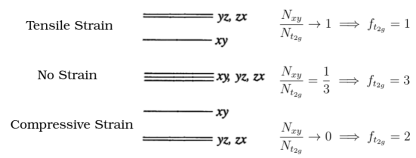
Figure 1: We show the three limiting cases for the $t_{2g}$ degeneracy. In the case without strain (middle panel), all the orbitals are degenerate ($f_{t_{2g}}$= 3). If strain is applied, degeneracy is broken towards having a lower lying singlet (tensile strain: $f_{t_{2g}}$= 1, top panel ) or a lower lying doublet (compressive strain: $f_{t_{2g}}$= 2, bottom panel ).

So we encounter that the factor $f_{t_{2g}}$ must be a function of $x=N_{xy}/N_{t_{2g}}$, its value must be contained in the interval $[1,3]$, and the maximum being equal to $3$ at $x=1/3$. Considering all these facts, we are going to fit the points shown in Fig. 1 to the following function (we chose a Gaussian because it is the simplest smooth function that one can think of that has only one adjustable extremum in the $[1,3]$ interval):

$$f_{t_{2g}}=\gamma+\frac{\alpha}{\beta\sqrt{\frac{\pi}{2}}}e^{-2\left(\frac{(x-1/3)}{\beta}\right)^{2}}$$ (17)

where the constants $\alpha$, $\beta$ and $\gamma$ are completely determined by the three limiting cases shown in Fig. 1.

A plot of the factor as a function of $x$ can be seen in Fig. 2 .

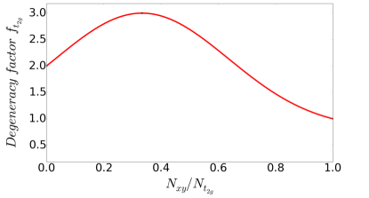
Figure 2: (Color online.)$f_{t_{2g}}$ function that results from eq. 17. This degeneracy factor fulfills the three limiting cases analyzed in Fig. 1 for the effect of strain in a t_2g electron system. It accounts for the orbital degeneracy of the system as a function of strain. N_xy and N${}_{t_{2g}}$ need to be determined ab initio.

We have found an analytical function for the high temperature thermopower from a statistical calculation. A degeneracy factor for the $t_{2g}$ was introduced as a function of $N_{xy}/N_{t_{2g}}$. This procedure will make possible to calculate the entropy-related term $S_{\left(T\rightarrow\infty\right)}$ from our DFT calculations just by computing $N_{xy}/N_{t_{2g}}$ for each strain introduced in the STO structure.

What we have done so far is being able to decouple the influence in thermopower variations with strain that come from electronic degeneracies and from band structure modifications such as effective mass changes, that strain will also introduce.

IV SrTiO₃ calculations

We have run calculations in SrTiO₃ simulating different strain situations by fixing the lattice parameter $a$ to that of the different standard perovskite substrates mentioned in the computational procedures section. For each $a$, we have optimized the lattice parameter $c$. We have not considered oxygen octahedral tilts, since this kind of distortions are hardly dependent on the impurity introduced as dopant. Therefore, we have limited our analysis to a cell volume distortion caused by biaxial strain. We have found that tensile (compressive) strain increases (reduces) the unit cell volume (see Fig. 6 in Appendix A). This has been experimentally reported previously for other oxides.Petrie et al. (2016)

With these structures we have performed electronic structure calculations including spin-orbit coupling with the TB-mBJ exchange-correlation potential, that allows to give an accurate band gap without additional computational cost. Band structure and density of states plots are shown in Fig. 7 in Appendix A for three different strain cases. We have found that the $t_{2g}$ bandwidth reduces with the unit cell volume and consequently with tensile strain (see Fig. 6 in Appendix A). This would have an implication on the effective mass because a reduced bandwidth leads to an increased average effective mass.

We have calculated the number of electrons in the $d_{xy}$ orbital, $N_{xy}$ and the total number of electrons in the $t_{2g}$ manifold, $N_{t_{2g}}$. Both values were obtained by integrating inside the Ti muffin-tin sphere. We will assume that the degree of localization will be identical for the three t_2g orbitals and hence integrating inside the muffin-tin spheres is sufficient for our purposes since we are only interested in the ratio. This ratio is needed to obtain the degeneracy factor $f_{t_{2g}}$ and consequently the thermopower at high temperature $S_{\left(T\rightarrow\infty\right)}$ as a function of doping.

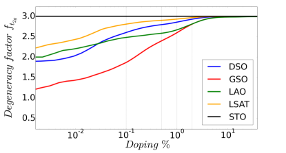
Figure 3: (Color online.) Degeneracy factor as a function of doping. In the low doping regime the degeneracy factors collapse to the three limiting cases exposed in Fig. 1, so they become largely dependent on strain. As we increase the doping level the factor becomes strain independent and tends to $3$ as the t_2g bands become more populated. Our calculations show that this occurs between 2-5 % Nb-doping. In the case of unstrained STO we see that the degeneracy factor is completely independent of the doping level since there is always a triple degeneracy in that case. This figure suggests that degeneracy effects vanish above about 5% doping.

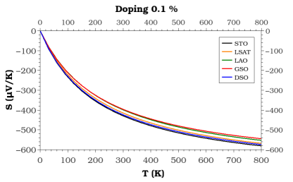
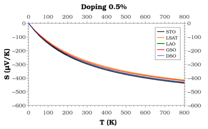
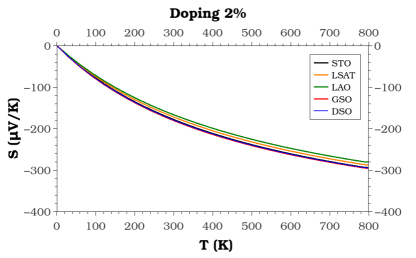
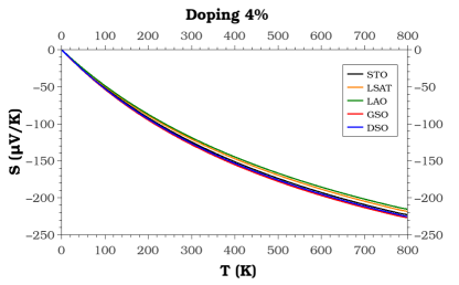
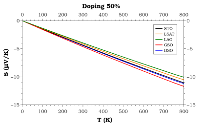
Figure 4: (Color online.) Representation of the Seebeck coefficient as a function of temperature using eq. (2) for six different doping regimes. The parameters obtained in each case are compiled in Table 2 in Appendix A. It can be seen that in the low doping regime (below 2.0%) the entropy-related term dominates the evolution with strain, leading to a reduction in the Seebeck coefficient (in magnitude) caused by any kind of strain. However, for high doping, it is the low temperature (energy-transport term) thermopower the one that dominates the strain tendency because $S_{\left(T\rightarrow\infty\right)}$ becomes strain independent (see Fig. 3). In that case, we see that tensile strain increases the thermopower (in magnitude).

Figure 3 shows the degeneracy factor dependence with doping for the different strain situations analyzed. We can see there, as a function of electron doping (in terms of electrons doped per unit cell, or Nb atoms substituting Ti, thus adding one extra electron to the conduction band per dopant). We can see that at low doping, the three limiting cases we discussed above are obtained (in the pure single ion picture), with the unstrained case having threefold degeneracy and the compressive or tensile strain cases tending to a twofold degenerate state or a singlet, respectively. As doping increases, the t_2g bands become more heavily populated and the actual band splittings become less and less important. Above 5% doping, the degeneracy factor becomes very close to 3, almost independent of strain. This illustrates that, even though in principle strain can tune degeneracies (by removing them), thermopower at high temperatures might not be affected if doping is substantial. This limit will of course depend on the system, but for STO we see that it is obtained (within a rigid band approximation) at values which are on the order of those sought for in the case of TE applications ($\sim$ 10²⁰ cm^-3). The important point to notice here is that the effect of strain on STO will not damage the TE efficiency at high temperature by reducing orbital degeneracies, when working at those high doping levels we are discussing.

Introducing these results of the degeneracy factor $f_{t_{2g}}$ in eq. (16), we can obtain the thermopower at high temperature $S_{\left(T\rightarrow\infty\right)}$ as a function of doping for the five strain situations that we are analyzing. Once $S_{\left(T\rightarrow\infty\right)}$ is computed, we have to solve the Boltzmann transport equations to obtain the parameter $A$. After that, we are in the position to get the value of $T_{0}$ using eq. (4) and consequently determine the three parameters of our model (eq. (2)). We must warn the reader that the Boltzmann transport equations used to compute the parameter $A$ would be less accurate at lower temperatures (in particular the phonon drag term is not included). Consequently, we will restrict our conclusions to analyze the evolution with strain and not focus too much on the actual values predicted for the thermopower. Also, discrepancies with experimental values could be due to the use of the constant relaxation time approximation which is used routinely but could have its limitations.Delugas et al. (2013)

Figure 4 shows six representations of the thermopower obtained using the model that we propose (eq. (2)) at different doping levels for the five strain cases analyzed, utilizing the values of the parameters that we have just calculated. The parameters $A$, $S_{\left(T\rightarrow\infty\right)}$, $T_{0}$ and also the obtained effective masses are summarized in Table 2 of Appendix A.

Figure 4 shows that the high temperature thermopower decreases in absolute value as we increase the doping level, as one would expect. Figure 5 shows the dependence that effective masses have with strain for the high doping regime. We can observe there that the theoretical effective masses obtained increase their value as doping increases. However, eq. (9) proposed to obtain the effective masses from parameter A is just a mechanism to get the effective mass tendency with strain. As we have said, it will only be valid in the high doping regime so we will focus on analyzing the evolution of the effective mass with strain but not so much on its actual doping dependence, since this will be quite dependent on the type of dopant. This feature is analyzed in Ref. Wunderlich et al., 2009 concluding that the effective mass will also depend on the kind of defect introduced to dope STO and the kind of distortions these introduce in the lattice.

Analyzing now each doping regime, we see that for low doping levels the strain tendency is given by the high temperature seebeck $S_{\left(T\rightarrow\infty\right)}$, i.e. we see in Fig. 4, for $0.1\%$ doping ($\sim 1.7\times 10^{19}$ cm^-3)that the Seebeck evolution with temperature follows the same strain dependence than $S_{\left(T\rightarrow\infty\right)}$. The unstrained case (with $a$ equal to that of STO) is the one that has the largest Seebeck value (in absolute value) at any temperature. Meanwhile, at high doping levels, greater than or equal to $2\%$, according to the results shown in Fig. 3, $S_{\left(T\rightarrow\infty\right)}$ stops being strain dependent. Consequently, the only dependence on strain in the evolution of the Seebeck with temperature comes from the $A$ parameter. We can easily check that the curves in the $2\%$, $4\%$ and $50\%$ doping levels ($\sim 3.3\times 10^{20}$, $\sim 6.6\times 10^{20}$ and $\sim 8.4\times 10^{21}$ cm^-3 respectively) follow the strain dependence given by parameter $A$ in Table 2, i.e., the inverse behaviour that effective masses have with strain (see Fig. 5). This comes about due to the fact that f${}_{t_{2g}}$ becomes very close to 3 and strain independent at those doping levels. Hence, the only changes to the thermopower occur via variations of the energy-transport term, in which (for high doping regimes $2\%$ or more) the thermopower is enhanced (in absolute value) by tensile strain.

Figure 5: (Color online.) Effective mass as a function of strain in the high doping regime. Effective mass increases (decreases) with tensile (compressive) strain and barely changes once all the bands become populated. The limit of 50% doping, even though beyond the validity of the rigid band approximation is shown as the limiting case found in LaAlO₃/STO interfaces.

For analyzing this dependence in detail, we have obtained the effective masses and its strain and doping dependence. Despite the fact that we show the effective masses calculated in the six cases (see table 2), it is hard to analyze its strain dependence away from the high doping limit. At $2\%$ doping, we can observe that the effective mass is larger for the unit cells with a larger volume (volume increases for tensile strain). Increasing the volume leads to a reduction in the hopping parameter, smaller band widths and hence a larger effective mass.Ohta et al. (2005) Above $2\%$ doping, such dependence with strain of the effective mass is retained. For lower doping values, the dependence with strain is more complex due to the partial involvement of different bands. The effective mass increases monotonously with doping and it reaches about 1.0 m₀ at about $50\%$ doping. In that doping region, a single parabolic band picture makes more sense than at low doping, where the sole concept of a single effective mass where all the bands contribute in a similar fashion is more difficult to identify.

In Ref. Janotti et al., 2011 Janotti et al. analyze the directional effective masses dependency with strain. In order to compare with their data, we can obtain a mean effective mass $m_{ave}^{*}$ performing a harmonic mean of the directional effective masses $m_{\Gamma-X}$ (parallel) and $m_{\Gamma-\overline{X}}$ (perpendicular to the strain direction) given in this article and we can compare these $m_{ave}^{*}$ with the effective masses we have obtained for $2.0\%$ doping, e.g. In our calculations LSAT corresponds to biaxial strain $-1.0\%$, STO $0.0\%$ and DSO $+1.0\%$. The results are summarized in Table 1. Their results, when analyzed this way, agree with ours in the strain dependence of the effective mass. However, the actual values are largely doping dependent, as we have discussed here.

Strain	$m_{\Gamma-X}$	$m_{\Gamma-\overline{X}}$	$m_{ave}^{*}$	Our $m^{*}$ ($2\%$ doping)
$-1.0\%$	0.67	0.40	0.547	0.672
$0.0\%$	0.55	0.55	0.550	0.700
$+1.0\%$	0.42	2.2	0.575	0.714

Table 1: Comparison between the effective masses obtained by A. Janotti et al. [Janotti et al., 2011] and the ones from our model at 2$\%$ doping. The masses are given in units of the free electron mass $m_{0}$. As we explain in the text, the actual values for the effective masses are largely doping dependent, but the evolution with strain we obtain is retained, and consistent with previous results in the literature.

The effective masses are slightly larger in our model than the ones provided in Ref. Janotti et al., 2011. We are comparing our calculations at $2.0\%$ doping level with the effective masses calculated from the inverse of the second derivative of the first conduction band in their case. However, the strain tendency is the same for both calculations. In view of the last two columns of Table 1 we can conclude that the mean effective mass in bulk STO increases (decreases) with positive (negative) biaxial strain. The same dependence is obtained in Ref. Wunderlich et al., 2009 where they found that an increase of the effective mass produces an increase of the thermopower.

A similar analysis to this one could be performed to check the Seebeck dependence with strain that we have obtained in our model. In Ref. Zou et al., 2013 Daifeng Zou et al. calculate the strain dependence of the thermopower in different directions (parallel and perpendicular to the strain plane). A harmonic mean value of their results provides the same strain dependence that we have obtained from our model, i.e., tensile strain enhances the thermopower.

The importance of the dependence of the Seebeck coefficient with strain is crucial when fine-tuning the TE properties of oxides, which often comes about due to nanostructurization, where strain is a key factor. This simple model we have put forward, supported by ab initio calculations, allows to account separately for the different factors that will influence the thermopower. In principle, one could naively think that applying strain simply destroys the t_2g degeneracy ruining the high temperature Seebeck coefficient, but we can see from our calculations on STO that this effect is small since the usual degrees of strain attained experimentally do not fully break the t_2g degeneracy, in particular at substantial doping ($\geq 10^{20}$ cm^-3), as is required for TE applications.Ohta et al. (2008) This is important in case one thinks of oxide-based design of new TE materials and wants to tune its thermopower with strain. We can see that the band effects such as band alignment modifications, doping levels and effective masses are much more important in affecting the Seebeck, and these need not act in a detrimental way for TE properties. Of course, the doping limit that leads to washing away the orbital degeneracies will be largely system-dependent.

V Concluding remarks

In conclusion, we have analyzed the thermopower in STO and its strain dependence for different n-doping levels and have been able to decouple the different origins of these dependencies: those coming from electronic degeneracies and entropy-related thermopower to those coming from the actual modifications in the band structures.

In the first part of this work, we have proposed a simplified model for the Seebeck coefficient. We consider the Kubo formalism and its temperature limits to build a simple equation for the thermopower based on the Mott formula. The first part of this equation corresponds to the energy-transport term and dominates in the low temperature regime. We obtain also a relationship between the free parameter of this term and a theoretical effective mass. The second term in our model corresponds to the entropy term at high temperatures, which is given by a Heikes-like equation. We introduce a degeneracy factor in this equation to model the effect of strain on the high temperature thermopower by affecting orbital degeneracies in the $t_{2g}$ manifold. We show how this degeneracy factor can be modeled by the use of ab initio calculations. Thus, we provide a way to model the Seebeck coefficient in a simple way by understanding how the effective mass and the electronic degeneracies evolve with strain. In the second part of the work, we have applied the model obtained in the first part to analyze the thermopower strain dependency of STO. We performed DFT-based calculations varying the lattice parameter $a$ matching it to that of five different usual substrates. The parameters that appear in our model were calculated for these five strain cases and for six different doping values. Thus, we obtained the thermopower as a function of temperature for different values of strain and doping. The results of our model can be summarized as follows: i) at low doping any type of strain will decrease the thermopower. This is caused by the dominance of the entropy-related term, since strain always reduces the degeneracy factor. ii) at high doping, the one useful for TE applications, starting at $2\%$ Nb-doping ($\sim 10^{20}$ cm^-3), the energy-transport term is dominant. Thus, at operating temperatures, tensile strain enhances the thermopower. In short, we have obtained that in the low doping regime the electron degeneracy dominates the Seebeck, while in the high doping regime the cell volume effect dominates (increasing volume leads to an increase in the Seebeck). In principle, this kind of reasoning can be extended to other oxides where orbital degeneracy plays a role. However, the particular results of a similar analysis such as the doping values of the various limits, will be largely system-dependent.

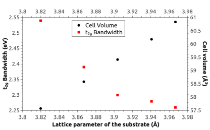
Appendix A

Figure 6: (Color online.) Bandwidth and unit cell volume for different strain situations. We see that bandwidth decreases with volume and volume is increased as positive (tensile) biaxial strain is applied.

In this Section we provide a few extra details for completeness of the electronic structure analysis. In Fig. 6 we plot the evolution of the unit cell volume with strain. We observe that, as discussed throughout the text, tensile strain leads to an increase in unit cell volume. The volume reduction that occurs for compressive strain leads to a smaller Ti-Ti distance, which increases the hopping integrals and hence leads to an increased bandwidth. This bandwidth increase should be related to a decrease in effective mass, as has been explained throughout the main text. Our analysis does not include, as we have also cautioned the readers, the specificities of the different types of dopants STO can sustain, we are only considering the pure effect of strain without the additional local distortions introduced by point defects and/or impurities.

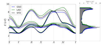
Figure 7: (Color online.) Band structure representation and density of states (DOS) calculated for different strain values. It can be seen how the bandwidth increases for compressive strain and decreases for tensile strain.

Figure 7 shows the band structures (only the conduction bands close to its bottom) for different strain situations together with the corresponding DOS’s on the same energy scale. GSO corresponds to the tensile strain limit and LAO to the compressive one. We can observe that the former leads, as explained above, to a reduction of the t_2g bandwidth, together with some shifts in the DOS peaks. The bottom of the conduction band is at $\Gamma$. We can see also that the position of the unoccupied t_2g bands is higher in energy for compressive strain and lower for the tensile strain case.

Table 2: Model’s parameters for the six representative doping values shown in Fig. 4. It is obtained that $S_{\left(T\rightarrow\infty\right)}$ decreases in absolute value if doping level increases. It can be seen that $S_{\left(T\rightarrow\infty\right)}$ is really strain dependent for low doping regimes while for the higher ones it becomes independent, which is in agreement with Fig. 3. Values for the effective masses $m^{*}/m_{0}$ obtained using eq. (9) are also shown. Only high doping rates, i.e. greater than or equal to $2.0\%$, can be considered relevant since it is where the free electron gas approximation can be taken as a good model. Effective mass is larger for tensile strain.

(a) Doping $\mathbf{0.1\%}$

	$A$ $(\mu V)$	$S_{\left(T\rightarrow\infty\right)}$ $(\mu V/K)$	$T_{0}$ $(K)$	$m^{*}/m_{0}$
GSO	163000	-703	232	0.145
DSO	158000	-730	217	0.150
STO	159000	-737	215	0.151
LSAT	166000	-730	228	0.145
LAO	174000	-720	242	0.140

(b) Doping $\mathbf{1.0\%}$

	$A$ $(\mu V)$	$S_{\left(T\rightarrow\infty\right)}$ $(\mu V/K)$	$T_{0}$ $(K)$	$m^{*}/m_{0}$
GSO	215000	-533	403	0.509
DSO	215000	-537	400	0.513
STO	219000	-545	403	0.506
LSAT	230000	-543	423	0.489
LAO	240000	-534	450	0.473

(c) Doping $\mathbf{4.0\%}$

	$A$ $(\mu V)$	$S_{\left(T\rightarrow\infty\right)}$ $(\mu V/K)$	$T_{0}$ $(K)$	$m^{*}/m_{0}$
GSO	296000	-425	696	0.932
DSO	303000	-426	711	0.917
STO	311000	-427	729	0.899
LSAT	325000	-427	761	0.870
LAO	330000	-425	775	0.868

(d) Doping $\mathbf{0.5\%}$

	$A$ $(\mu V)$	$S_{\left(T\rightarrow\infty\right)}$ $(\mu V/K)$	$T_{0}$ $(K)$	$m^{*}/m_{0}$
GSO	195000	-592	329	0.353
DSO	199000	-605	323	0.348
STO	190000	-609	312	0.368
LSAT	199000	-607	328	0.354
LAO	210000	-596	352	0.341

(e) Doping $\mathbf{2.0\%}$

	$A$ $(\mu V)$	$S_{\left(T\rightarrow\infty\right)}$ $(\mu V/K)$	$T_{0}$ $(K)$	$m^{*}/m_{0}$
GSO	241000	-481	501	0.720
DSO	245000	-483	508	0.714
STO	252000	-486	519	0.700
LSAT	265000	-485	546	0.672
LAO	272000	-481	567	0.661

(f) Doping $\mathbf{50.0\%}$

	$A$ $(\mu V)$	$S_{\left(T\rightarrow\infty\right)}$ $(\mu V/K)$	$T_{0}$ $(K)$	$m^{*}/m_{0}$
GSO	1490000	-154	9690	0.995
DSO	1560000	-154	10100	0.957
STO	1590000	-154	10300	0.949
LSAT	1670000	-154	10900	0.910
LAO	1750000	-154	11400	0.878

Table 2 summarizes the results of the fit to our model (different parameters described in detail in the main text) for the thermopower at different doping levels and for the various strain situations considered.

References

- Ohtomo and Hwang (2004) A. Ohtomo and H. Hwang, Nature 427, 423 (2004).
- López-Quintela et al. (2003) M. A. López-Quintela, L. E. Hueso, J. Rivas, and F. Rivadulla, Nanotechnology 14, 212 (2003).
- Maeng et al. (2008) J. Maeng, T.-W. Kim, G. Jo, and T. Lee, Mat. Res. Bull. 43, 1649 (2008).
- Mannhart and Schlom (2010) J. Mannhart and D. G. Schlom, Science 327, 1607 (2010).
- Limelette et al. (2005) P. Limelette, V. Hardy, P. Auban-Senzier, D. Jérome, D. Flahaut, S. Hébert, R. Frésard, C. Simon, J. Noudem, and A. Maignan, Phys. Rev. B 71, 233108 (2005).
- Terasaki et al. (1997) I. Terasaki, Y. Sasago, and K. Uchinokura, Phys. Rev. B 56, R12685 (1997).
- Moos et al. (1995) R. Moos, A. Gnudi, and K. H. Härdtl, Journal of Applied Physics 78, 5042 (1995).
- Ohta et al. (2007) H. Ohta, S. Kim, Y. Mune, T. Mizoguchi, K. Nomura, S. Ohta, T. Nomura, Y. Nakanishi, Y. Ikuhara, M. Hirano, et al., Nat. Mat. 6, 129 (2007).
- Snyder and Toberer (2008) G. J. Snyder and E. S. Toberer, Nat. Mater. 7, 105 (2008).
- Lu et al. (2016) Z. Lu, H. Zhang, W. Lei, D. C. Sinclair, and I. M. Reaney, Chemistry of Materials 28, 925 (2016).
- Zheng et al. (2013) G. H. Zheng, Z. H. Yuan, Z. X. Dai, H. Q. Wang, H. B. Li, Y. Q. Ma, and G. Li, Journal of Low Temperature Physics 173, 80 (2013).
- Yu et al. (2008) C. Yu, M. L. Scullin, M. Huijben, R. Ramesh, and A. Majumdar, Applied Physics Letters 92, 191911 (2008).
- Dresselhaus et al. (2007) M. Dresselhaus, G. Chen, M. Tang, R. Yang, H. Lee, D. Wang, Z. Ren, J.-P. Fleurial, and P. Gogna, Advanced Materials 19, 1043 (2007).
- Li et al. (2010) X. Li, K. Maute, M. L. Dunn, and R. Yang, Phys. Rev. B 81, 245318 (2010).
- Pardo et al. (2013) V. Pardo, A. S. Botana, and D. Baldomir, Phys. Rev. B 87, 125148 (2013).
- Chen et al. (2003) J. Chen, S. Z. Deng, N. S. Xu, W. Zhang, X. Wen, and S. Yang, Applied Physics Letters 83, 746 (2003).
- Imada et al. (1998) M. Imada, A. Fujimori, and Y. Tokura, Rev. Mod. Phys. 70, 1039 (1998).
- Qiao et al. (2011) Q. Qiao, A. Gulec, T. Paulauskas, S. Kolesnik, B. Dabrowski, M. Ozdemir, C. Boyraz, D. Mazumdar, A. Gupta, and R. F. Klie, Journal of Physics: Condensed Matter 23, 305005 (2011).
- Sarantopoulos et al. (2015) A. Sarantopoulos, E. Ferreiro-Vila, V. Pardo, C. Magén, M. H. Aguirre, and F. Rivadulla, Phys. Rev. Lett. 115, 166801 (2015).
- Villar Arribi et al. (2016) P. Villar Arribi, P. García-Fernández, J. Junquera, and V. Pardo, arxiv/1602.01539 (2016).
- Hohenberg and Kohn (1964) P. Hohenberg and W. Kohn, Phys. Rev. 136, B864 (1964).
- Kohn and Sham (1965) W. Kohn and L. J. Sham, Phys. Rev. 140, A1133 (1965).
- Schwarz and Blaha (2003) K. Schwarz and P. Blaha, Comp. Mater. Sci. 28, 259 (2003).
- Wu and Cohen (2006) Z. Wu and R. E. Cohen, Phys. Rev. B 73, 235116 (2006).
- Tran and Blaha (2009) F. Tran and P. Blaha, Phys. Rev. Lett. 102, 226401 (2009).
- Koller et al. (2011) D. Koller, F. Tran, and P. Blaha, Phys. Rev. B 83, 195134 (2011).
- Dixit et al. (2012) H. Dixit, R. Saniz, S. Cottenier, D. Lamoen, and B. Partoens, J. Phys.: Condens. Matter 24, 205503 (2012).
- Singh and Nordstrom (2006) D. J. Singh and L. Nordstrom, Planewaves, Pseudopotentials, and the LAPW method (Springer Science & Business Media, 2006).
- Madsen and Singh (2006) G. K. H. Madsen and D. J. Singh, Comp. Phys. Comm. 175, 67 (2006).
- Hayward et al. (2005) S. A. Hayward, F. D. Morrison, S. A. T. Redfern, E. K. H. Salje, J. F. Scott, K. S. Knight, S. Tarantino, A. M. Glazer, V. Shuvaeva, P. Daniel, M. Zhang, and M. A. Carpenter, Phys. Rev. B 72, 054110 (2005).
- Wong et al. (2010) F. J. Wong, S.-H. Baek, R. V. Chopdekar, V. V. Mehta, H.-W. Jang, C.-B. Eom, and Y. Suzuki, Phys. Rev. B 81, 161101 (2010).
- Kubo et al. (1957) R. Kubo, M. Yokota, and S. Nakajima, Journal of the Physical Society of Japan 12, 1203 (1957), http://dx.doi.org/10.1143/JPSJ.12.1203 .
- Chaikin and Beni (1976) P. M. Chaikin and G. Beni, Phys. Rev. B 13, 647 (1976).
- Janotti et al. (2011) A. Janotti, D. Steiauf, and C. G. Van de Walle, Physical Review B 84, 201304 (2011).
- Fritzsche (1971) H. Fritzsche, Solid State Communications 9, 1813 (1971).
- Kittel (2004) C. Kittel, Introduction to Solid State Physics, 8th ed. (Wiley, 2004).
- Petrie et al. (2016) J. R. Petrie, C. Mitra, H. Jeen, W. S. Choi, T. L. Meyer, F. A. Reboredo, J. W. Freeland, G. Eres, and H. N. Lee, Advanced Functional Materials 26, 1564 (2016).
- Delugas et al. (2013) P. Delugas, A. Filippetti, M. J. Verstraete, I. Pallecchi, D. Marré, and V. Fiorentini, Phys. Rev. B 88, 045310 (2013).
- Wunderlich et al. (2009) W. Wunderlich, H. Ohta, and K. Koumoto, Physica B: Condensed Matter 404, 2202 (2009).
- Ohta et al. (2005) S. Ohta, T. Nomura, H. Ohta, M. Hirano, H. Hosono, and K. Koumoto, Applied Physics Letters 87, 092108 (2005).
- Zou et al. (2013) D. Zou, Y. Liu, S. Xie, J. Lin, and J. Li, Chemical Physics Letters 586, 159 (2013).
- Ohta et al. (2008) H. Ohta, K. Sugiura, and K. Koumoto, Inorganic Chemistry 47, 8429 (2008).