Bose-Einstein correlations and $\mathbf{v_{2n}}$ and $\mathbf{v_{2n-1}}$ in hadron and nucleus collisions

Abstract

We show that Bose-Einstein correlations of identical particles in hadron and nucleus high energy collisions, lead to long range rapidity correlations in the azimuthal angle. These correlations are inherent features of the CGC/saturation approach, however, their origin is more general than this approach. In framework of the proposed technique both even and odd $v_{n}$ occur naturally, independent of the type of target and projectile. We are of the opinion that it is premature to conclude that the appearance of azimuthal correlations are due to the hydrodynamical behaviour of the quark-gluon plasma.

One of the most intriguing experimental observations made at the LHC and RHIC, is the occurrence of the same pattern of azimuthal angle correlations in the three types of interactions: hadron-hadron, hadron-nucleus and nucleus-nucleus collisions. In all three reactions, correlations in the events with large density of produced particles, are observed between two charged hadrons, which are separated by large values of rapidity CMSPP ; STARAA ; PHOBOSAA ; STARAA1 ; CMSPA ; CMSAA ; ALICE and these correlations do not depend on the rapidity separation of the particles. Due to causality argumentsCAUSALITY , two hadrons with large difference in rapidity between them, could only correlate at the early stage of the collision and, therefore, we expect that the correlations between two particles with large rapidity difference (at least the correlations in rapidity) are due to the partonic state with large parton density. The CGC/saturation approach (see KOLEB for a review) appears to be a natural candidate for the description of these correlations, as these correlations are strong in the dense colliding systems. However, unlike the large rapidity correlations, the azimuthal angle correlations can originate from the collective flow in the final state FINSTATE . At first sight, this source appears even more plausible, since $v_{n}$ with odd $n$ do not appear in the CGC/saturation approach.

In this article we show that the long range rapidity correlations in the azimuthal angle, arise naturally from the Bose-Einstein correlations of produced identical particle in high energy collisions. They originate from the initial state wave function of the colliding particles, and they are features characteristic of the CGC/saturation approach. However, their occurrence is more general, and can be estimated in other frameworks. The long range rapidity correlations stem from the production of two parton showers in QCD (see Fig. 1). The structure of the parton shower in QCD is described by the exchange of the BFKL Pomeron, while the upper and low blobs in Fig. 1-b require modeling, due to our poor theoretical knowledge of the confinement of quarks and gluons. However, if two produced gluons have the same quantum numbers, we need to take into account an additional Mueller diagramMUDI of Fig. 2-b in which two gluons with $(y_{1},\boldsymbol{p}_{T2})$ and $(y_{2},\boldsymbol{p}_{T1})$ are produced. When $\boldsymbol{p}_{T1}\,\to\,\boldsymbol{p}_{T2}$ the two production processes become identical, leading to the cross section $\sigma\left(\mbox{two identical gluons}\right)=2\sigma\left(\mbox{two different gluons}\right)$, as one expects. However, when $|\boldsymbol{p}_{T2}-\boldsymbol{p}_{T1}|\gg 1/R$ where $R$ is the size of the emitter, the interference diagram becomes small and can be neglected.

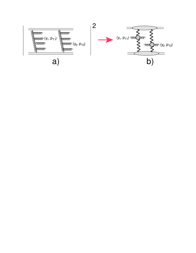
Figure 1: Production of two gluons with $(y_{1},\boldsymbol{p}_{T1})$ and $(y_{2},\boldsymbol{p}_{T2})$ in two parton showers (Fig. 1-a). Fig. 1-b shows the double inclusive cross section in Mueller diagram technique MUDI . The wavy lines denote the BFKL Pomerons

At first sight the Mueller diagram of Fig. 2-b in general case $y_{1}\neq y_{2}$ and $\boldsymbol{p}_{T1}\neq\boldsymbol{p}_{T2}$ looks problematic, since it describes the interference between two different final states. However, in the leading log(1/x) approximation(LLA) of perturbative QCD $\left(\bar{\alpha}_{S}\left(Y-y_{1}\right)\right)^{n_{1}},\left(\bar{\alpha}_{S}\left(y_{1}-0\right)\right)^{n_{2}},\left(\bar{\alpha}_{S}\left(Y-y_{2}\right)\right)^{n_{3}}$ and $\left(\bar{\alpha}_{S}\left(y_{2}-0\right)\right)^{n_{4}}$ contributions stem from the integration of the phase space which for the gluon $(i)$ has the following form: $dy_{1}d^{2}p_{Ti}$. In LLA we have the following ordering (for two parton showers production):

first parton shower $$\rightarrow Y\,>\,\dots\,>\,y_{i}\,>\,\dots\,>\,y_{n_{1}}\,>\,y_{1}\,>\,y_{n_{2}}\,>\,\dots\,>\,y_{i}\,>\,\dots\,>0;$$

second parton shower $$\rightarrow Y\,>\,\dots\,>\,y_{i}\,>\,\dots\,>\,y_{n_{3}}\,>\,y_{2}\,>\,y_{n_{4}}\,>\,\dots\,>\,y_{i}\,>\,\dots\,>0;$$ (1)

Integrating over $y_{i}$ and neglecting $y_{i}$ dependence of the production amplitude BFKL ; LI we obtain the contribution

$$\frac{d\sigma^{\rm different\,gluons}}{dy_{1}d^{2}p_{T1}\,dy_{2}\,d^{2}p_{T2}}\,\, = \,\,\sum^{\infty}_{n_{1}+n_{2}-2>2}\,\,\sum^{\infty}_{n_{3}+n_{4}-2>2}\,\int d\Phi^{(1)}_{n_{1}+n_{2}}d\Phi^{(2)}_{n_{3}+n_{4}}\,|A^{\rm different\,gluons}\left(\{y_{i},p_{Ti}\};y_{1},p_{T1};y_{2},p_{T2}\right)|^{2}$$ (2)

$$= \sum^{\infty}_{n_{1}+n_{2}-2>2}\,\,\sum^{\infty}_{n_{3}+n_{4}-2>2}\underbrace{\frac{\left(\bar{\alpha}_{S}\left(Y-y_{1}\right)\right)^{n_{1}}}{n_{1}!}\,\frac{\left(\bar{\alpha}_{S}\left(y_{1}-0\right)\right)^{n_{2}}}{n_{2}!}\,\frac{\left(\bar{\alpha}_{S}\left(Y-y_{2}\right)\right)^{n_{3}}}{n_{3}!}\,\frac{\left(\bar{\alpha}_{S}\left(y_{2}-0\right)\right)^{n_{4}}}{n_{4}!}}_{\rm integral\,\,over\,\,lomitudinal\,\,phase\,\,space}$$

$$\times \int\prod_{i}d^{2}p_{Ti}\,\,|A^{\rm different\,gluons}\left(\{y_{i}=0,p_{Ti}\};y_{1}=0,p_{T1};y_{2}=0,p_{T2}\right)\|^{2}$$

where $d\Phi^{(1)}_{n_{1}+n_{2}}$ and $d\Phi^{(2)}_{n_{3}+n_{4}}$ denote the phase space of the produced gluons in the first and second parton showers.

Eq. (2) represents the factorization of the longitudinal and transverse degrees of freedom, which is the principle characteristic of the LLABFKL ; LI .

For two parton showers the production amplitude $A^{\rm different\,gluons}\left(\{y_{i}=0,p_{Ti}\};y_{1}=0,p_{T1};y_{2}=0,p_{T2}\right)\,\propto\,A^{(1)}_{n_{1}n_{2}}\left(\{y_{i}=0,p_{Ti}\};y_{1}=0,p_{T1}\right)\,A^{(2)}_{n_{3}n_{4}}\left(\{y_{i}=0,p_{Ti}\};y_{2}=0,p_{T2}\right)$. Summing over $n_{i}$, we obtain the Mueller diagram of Fig. 1-b.

For identical particles we need to replace

$$A^{\rm different\,gluons}\left(\{y_{i}=0,p_{Ti}\};y_{1}=0,p_{T1};y_{2}=0,p_{T2}\right)\,\propto$$

$$\,A^{(1)}_{n_{1}n_{2}}\left(\{y_{i}=0,p_{Ti}\};y_{1}=0,p_{T1}\right)\,A^{(2)}_{n_{3}n_{4}}\left(\{y_{i}=0,p_{Ti}\};y_{2}=0,p_{T2}\right)\,\,\longrightarrow$$ (3)

$$A^{\rm identical\,gluons}\left(\{y_{i}=0,p_{Ti}\};y_{1}=0,p_{T1};y_{2}=0,p_{T2}\right)\,=\,$$

$$A^{\rm different\,gluons}\left(\{y_{i}=0,p_{Ti}\};y_{1}=0,p_{T1};y_{2}=0,p_{T2}\right)\,\,+\,\,A^{\rm different\,gluons}\left(\{y_{i}=0,p_{Ti}\};y_{2}=0,p_{T2};y_{1}=0,p_{T1}\right)\propto$$

$$A^{(1)}_{n_{1}n_{2}}\left(\{0,p_{Ti}\};0,p_{T1}\right)\,A^{(2)}_{n_{3}n_{4}}\left(\{0,p_{Ti}\};0,p_{T2}\right)\,\,+\,\,A^{(1)}_{n_{1}n_{2}}\left(\{0,p_{Ti}\};0,p_{T2}\right)\,A^{(2)}_{n_{3}n_{4}}\left(\{0,p_{Ti}\};0,p_{T1}\right)$$

We note that in Eq. (Bose-Einstein correlations and $\mathbf{v_{2n}}$ and $\mathbf{v_{2n-1}}$ in hadron and nucleus collisions) we use the Bose-Einstein symmetry for the amplitudes which depend only on the transverse momenta of produced particles. Summing over $n_{i}$, we obtain the contributions which are shown in Fig. 2-a and Fig. 2-b.

Estimates in the LLA, which we discussed above, are performed in the kinematic region where $\bar{\alpha}_{S}\left(y_{k}-y_{m}\right)\,\geq 1$ ($y_{k}(y_{m})=y_{0},y_{1},y_{2},y_{4}=Y$ with $y_{0}=0$ ) including $\bar{\alpha}_{S}\left(y_{1}-y_{2}\right)\,\geq 1$). Note that the calculations of Ref.KOLUCOR , were done for $\bar{\alpha}_{S}\left(y_{1}-y_{2}\right)\,\leq\,1$.

The angular correlation stems from the diagram of Fig. 2-b in which the upper BFKL Pomerons carry momentum $\boldsymbol{k}-\boldsymbol{p}_{T,12}$ with $\boldsymbol{p}_{T,12}\,=\,\boldsymbol{p}_{T1}\,-\,\boldsymbol{p}_{T2}$, while the lower BFKL Pomerons have momenta $\boldsymbol{k}$. In this article we demonstrate a mechanism for the appearance of these angular correlations in the framework of a simple approach: the soft Pomeron calculus. The Mueller diagrams for the correlation between two $\pi^{-}$ are shown in Fig. 3. As can be seen from Fig. 3 we use the eikonal model for estimates of the amplitude for two soft Pomeron production. In the case of the nucleus target and/or projectile, this model corresponds to the Glauber model.

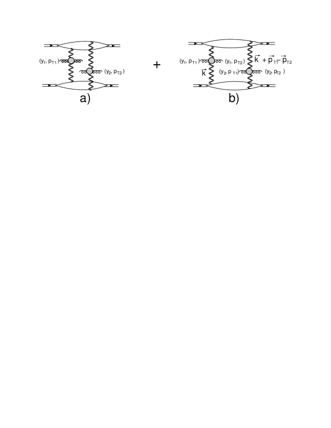
Figure 2: Production of two identical gluons with $(y_{1},\boldsymbol{p}_{T1})$ and $(y_{2},\boldsymbol{p}_{T2})$ in two parton showers. The diagrams in the Mueller diagram technique MUDI are shown in Fig. 2-a and Fig. 2-b. The wavy lines denote the BFKL PomeronsBFKL ; LI .

For the vertices of the soft Pomeron interaction with the projectile and target we use the following parametrizations:

$$g_{pr}\left(k^{2}\right)\,=\,g^{0}_{pr}\,e^{-\frac{1}{2}B_{pr}\,k^{2}_{T}};~{}~{}~{}~{}~{}~{}~{}~{}g_{tr}\left(k^{2}\right)\,=\,g^{0}_{tr}\,e^{-\frac{1}{2}B_{tr}\,k^{2}_{T}};$$ (4)

and for the vertex of pion emission from the Pomeron we use the simplest parametrization:

$$a_{{I\!\!P}{I\!\!P}}\left(p_{T1},p_{T2}\right)\,=\,a^{0}_{{I\!\!P}{I\!\!P}}\,e^{-\frac{1}{2}B_{e}\,\left(p^{2}_{T1}\,+\,p^{2}_{T2}\right)}$$ (5)

We have neglected the possible dependence of $a_{{I\!\!P}{I\!\!P}}$ on $k^{2}$ and $\boldsymbol{p}_{T,12}$.

Figure 3: The Mueller diagrams for production of two identical $\pi^{-}$ with $(y_{1},\boldsymbol{p}_{T1})$ and $(y_{2},\boldsymbol{p}_{T2})$ in two parton showers (see Fig. 3-a - Fig. 3-c). The diagram of Fig. 3-d describes the inclusive production of pions. The zigzag lines denote the soft Pomerons.

The contribution of Fig. 3-c to the double inclusive cross section is equal to

$$\frac{d\sigma}{dy_{1}d^{2}p_{T1}\,dy_{2}\,d^{2}p_{T2}}\,\, = \,\,a^{2}_{{I\!\!P}{I\!\!P}}\left(p_{T1},p_{T2}\right)\,e^{2\Delta_{I\!\!P}Y}\,\frac{\left(g^{0}_{pr}\right)^{2}\,\left(g^{0}_{tr}\right)^{2}}{4\pi^{2}}\int d^{2}k_{T}\,\exp\Big{(}-B_{tr}\,k^{2}_{T}\,-B_{pr}\left(\boldsymbol{k}_{T}-\boldsymbol{p}_{T,12}\right)^{2}\Big{)}\,$$

$$= \,\left(a^{0}_{{I\!\!P}{I\!\!P}}\right)^{2}\frac{\left(g^{0}_{pr}\right)^{2}\,\left(g^{0}_{tr}\right)^{2}}{4\pi\,\left(B_{tr}+B_{pr}\right)}\,e^{2\Delta_{I\!\!P}Y}\,\exp\Big{(}-\left(B_{e}+B_{R}\right)\,\left(p^{2}_{T1}\,+\,p^{2}_{T2}\right)\,-\,2\,B_{R}\,p_{T1}p_{T2}\cos\left(\varphi\right)\Big{)}\vspace{0.2cm}$$

where

$$B_{R}\,\,=\,\,\frac{B_{pr}\,B_{tr}}{B_{pr}\,+\,B_{tr}}$$ (7)

and $\Delta_{I\!\!P}$ is the intercept of the soft Pomeron. The sum of all diagrams of Fig. 3 leads to

$$\frac{d\sigma}{dy_{1}d^{2}p_{T1}\,dy_{2}\,d^{2}p_{T2}}\,\,=\,\,$$ (8)

$$\left(a^{0}_{{I\!\!P}{I\!\!P}}\right)^{2}\frac{\left(g^{0}_{pr}\right)^{2}\,\left(g^{0}_{tr}\right)^{2}}{4\pi\,\left(B_{tr}+B_{pr}\right)}\,e^{2\Delta_{I\!\!P}Y}\,\exp\Big{(}-B_{e}\,\left(p^{2}_{T1}\,+\,p^{2}_{T2}\right)\Big{)}\,\Bigg{\{}1\,\,+\,\,\exp\Big{(}\,-\,B_{R}\,\left(p^{2}_{T1}\,\,-2\,p_{T1}p_{T2}\cos\left(\varphi\right)\,+\,p^{2}_{T2}\right)\Big{)}\Bigg{\}}$$

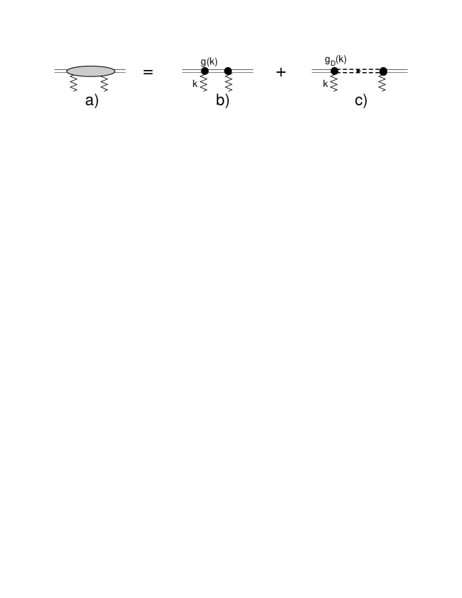
Figure 4: The structure of the Pomeron-proton amplitude: Fig. 4-b is the contribution of the eikonal approach,Fig. 4-c is the diffraction dissociation contribution.

The expansion of Eq. (8) contains all powers of $\cos\left(\varphi\right)$, or in other words, all $\cos\left(n\,\varphi\right)$ with even and odd $n$. The other feature of Eq. (8) is that the double inclusive cross section does not depend on $y_{1}$ and $y_{2}$, displaying the long rapidity correlations

We can re-write Eq. (8) in terms of the observables which can be measured: the slopes of elastic scattering and the rapidity correlation function $C\left(y_{1},y_{2}\right)$ defined as

$$C\left(y_{1},y_{2}\right)\,\,=\,\,\frac{1}{\sigma_{in}}\,\int d^{2}p_{T1}\,d^{2}p_{T2}\,\frac{d\sigma}{dy_{1}d^{2}p_{T1}\,dy_{2}\,d^{2}p_{T2}}\Bigg{/}\left(\frac{1}{\sigma_{in}}\,\int d^{2}p_{T1}\,\frac{d\sigma}{dy_{1}d^{2}p_{T1}}\right)\,\left(\frac{1}{\sigma_{in}}\,\int d^{2}p_{T2}\,\frac{d\sigma}{dy_{2}d^{2}p_{T,2}}\right)$$ (9)

It is more convenient to introduces a correlation function $C\left(y_{1},p_{T1};y_{2},p_{T2}\right)$ as

$$C\left(y_{1},p_{T1};y_{2},p_{T2}\right)\,=\,\,\frac{\frac{1}{\sigma_{in}}\frac{d\sigma}{dy_{1}d^{2}p_{T1}\,dy_{2}\,d^{2}p_{T2}}}{\left(\frac{1}{\sigma_{in}}\,\,\frac{d\sigma}{dy_{1}d^{2}p_{T1}}\right)\,\left(\frac{1}{\sigma_{in}}\,\frac{d\sigma}{dy_{2}d^{2}p_{T2}}\right)}$$ (10)

$$=\,C\left(y_{1},y_{2}\right)\,\Bigg{\{}1\,\,+\,\,\frac{B_{R}}{B_{R}+B_{e}}\exp\Big{(}\,-\,B_{R}\,\left(p^{2}_{T1}\,\,-2\,p_{T1}p_{T2}\cos\left(\varphi\right)\,+\,p^{2}_{T2}\right)\Big{)}\Bigg{\}}$$

Using

$$\int^{2\pi}_{0}d\varphi\,e^{2\,p_{T1}p_{T2}\cos\left(\varphi\right)}\,\cos\left(n\,\varphi\right)\,=\,\,2\,\pi\,I_{n}\left(2\,p_{T1}p_{T2}\right),$$ (11)

where $I_{n}\left(z\right)$ is the modified Bessel function of the first kind, we will decompose the term in $\{\dots\}$ in $C\left(y_{1},p_{T1};y_{2},p_{T2}\right)$ into Fourier modes in the relative azimuthal angle $\varphi$ between two produced pions:

$$C\left(y_{1},p_{T1};y_{2},p_{T2}\right)\,\propto\,1\,\,+\,\,2\,\sum_{n=1}\,V_{n\Delta}\left(p_{T1},p_{T2}\right)\,\cos\left(n\varphi\right)$$

$$\mbox{with}~{}~{}V_{n\Delta}\left(p_{T1},p_{T2}\right)\,=\,\frac{1}{2}I_{n}\left(2\,B_{R}\,p_{T1}\,p_{T2}\right)\frac{e^{-\,B_{R}\,\left(p^{2}_{T1}+p^{2}_{T2}\right)}}{1\,+\,I_{0}\left(2\,B_{R}\,p_{T1}\,p_{T2}\right)e^{-\,B_{R}\,\left(p^{2}_{T1}+p^{2}_{T2}\right)}}$$ (12)

assuming that $B_{e}\,\ll\,B_{R}$.

The coefficients $v_{n}\left(p_{T}\right)$ are equal to

$$v_{n}\left(p_{T}\right)\,=\,\frac{V_{n\Delta}\left(p_{T},p^{\mbox{\footnotesize Ref}}_{T}\right)}{\sqrt{V_{n\Delta}\left(p^{\mbox{\footnotesize Ref}}_{T},p^{\mbox{\footnotesize Ref}}_{T}\right)}}\,=\,\frac{1}{\sqrt{2}}\frac{I_{n}\left(2\,B_{R}\,p_{T1}\,p^{\mbox{\footnotesize Ref}}_{T2}\right)}{\sqrt{I_{n}\left(2\,B_{R}\,\left(\,p^{\mbox{\footnotesize Ref}}_{T2}\right)^{2}\right)}}\,\frac{\sqrt{1\,+\,I_{0}\left(2\,B_{R}\,\left(p^{\mbox{\footnotesize Ref}}_{T2}\right)^{2}\right)e^{-\,2\,B_{R}\,\left(p^{\mbox{\footnotesize Ref}}_{T2}\right)^{2}}}}{1\,+\,I_{0}\left(2\,B_{R}\,p_{T1}\,p^{\mbox{\footnotesize Ref}}_{T2}\right)e^{-\,B_{R}\,\left(p^{2}_{T1}+\left(p^{\mbox{\footnotesize Ref}}_{T2}\right)^{2}\right)}}$$ (13)

where the value of $p^{\mbox{\footnotesize Ref}}_{T}$ is determined by the experimental procedure. Fixing $p^{\mbox{\footnotesize Ref}}_{T}=p_{T}$ we obtain

$$v_{n}\left(p_{T}\right)\,=\,\frac{1}{\sqrt{2}}\,e^{-B_{R}\,p^{2}_{T}}\sqrt{\frac{I_{n}\left(2\,B_{R}\,p^{2}_{T}\right)}{1\,+\,I_{0}\left(2\,B_{R}\,p^{2}_{T}\right)e^{-\,2\,B_{R}\,p^{2}_{T}}}}$$ (14)

Eq. (14) stems from the diagrams of Fig. 3. However like-sign pion pairs contribute a third of total contribution to pion pair production. This means that the double inclusive cross section is equal to

$$\frac{d\sigma}{dy_{1}d^{2}p_{T1}\,dy_{2}\,d^{2}p_{T2}}\,\, = \,\,\frac{d\sigma}{dy_{1}d^{2}p_{T1}\,dy_{2}\,d^{2}p_{T2}}\left(\rm unlike\,pairs\right)\,\,+\,\,\frac{d\sigma}{dy_{1}d^{2}p_{T1}\,dy_{2}\,d^{2}p_{T2}}\left(\rm identical\,pairs\right)\,\,$$ (15)

$$= \,\,\frac{d\sigma}{dy_{1}d^{2}p_{T1}\,dy_{2}\,d^{2}p_{T2}}\left(\rm unlike\,pairs\right)\,\,\Big{(}1\,+\,\frac{1}{3}C\left(p_{T1};p_{T2}\right)\Big{)}$$

Therefore, Eq. (14) has to be multiplied by factor $1/3$.

In Eq. (7) $B_{pr}$ and $B_{tr}$ can be expressed in terms of the slope for elastic cross section for projectile-projectile and target -target scattering, respectively: $B_{pr}=\frac{1}{2}B^{\rm el}_{\rm pr\,-\,pr}$ and $B_{tr}=\frac{1}{2}B^{\rm el}_{\rm tr\,-\,tr}$.

For proton-proton scattering at W = 7  GeV, $B_{pr}=B_{tr}=\frac{1}{2}B^{\rm el}_{\rm p\,-\,p}\,=\,10\,GeV^{-2}$ TOTEM , which lead to $B_{R}\,=\,5\,GeV^{-2}$. Plugging this value in Eq. (14) we obtain the $v_{n}$ shown in Fig. 5. One can see that we obtain sufficiently large values of $v_{n}$, which are concentrated at rather large values of $p_{T}$. The width of $p_{T}$ distribution will increase if we include a more complicated structure of the Pomeron-hadron amplitude (see Fig. 4) and include diffraction dissociation processes (see Fig. 4-c), parametrizing $g_{B}(k)=g^{0}_{D}\exp\left(-hB_{D}\,k^{2}\right)$; Eq. (14) will have the following form:

$$v_{n}\left(p_{T}\right)\,=\,\frac{1}{3\,\sqrt{2}}\,\ \sqrt{\frac{I_{n}\left(2\,B_{R}\,p^{2}_{T}\right)\,e^{-2\,B_{R}\,p^{2}_{T}}\,\,+\,\,\frac{\sigma_{sd}\,B^{sd}_{D}}{\sigma_{el}\,B^{el}}\,I_{n}\left(2\,B_{D}\,p^{2}_{T}\right)\,e^{-2\,B_{D}\,p^{2}_{T}}}{1\,+\,I_{0}\left(2\,B_{R}\,p^{2}_{T}\right)e^{-\,2\,B_{R}\,p^{2}_{T}}\,\,+\,\,\frac{\sigma_{sd}\,B^{sd}_{D}}{\sigma_{el}\,B^{el}}I_{0}\left(2\,B_{D}\,p^{2}_{T}\right)e^{-\,2\,B_{D}\,p^{2}_{T}}}}$$ (16)

where $\sigma_{sd}$ denotes the cross section of the single diffractive production, $B^{sd}_{D}$ the slope of the differential cross section for diffraction dissociation is roughly equal to $\frac{1}{2}B^{el}$, and $B_{D}$ is the slope of Pomeron-hadron vertex for diffraction dissociation (see Fig. 4-c). The value of $B_{D}$ has been evaluated in Ref.KOTE , and it is equal $\approx 1\,GeV^{-2}$. Fig. 5-b shows the calculation using Eq. (16) with $\frac{\sigma_{sd}\,B^{sd}_{D}}{\sigma_{el}\,B^{el}}$. One can see that the $p_{T}$ distribution becomes broader.

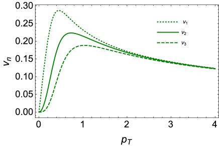
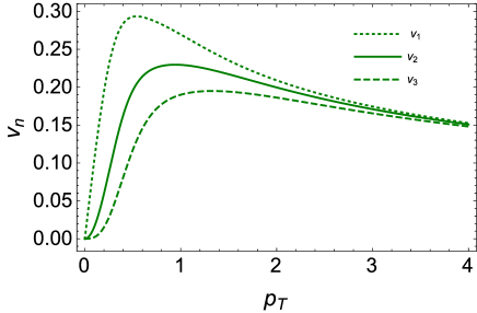
Fig. 5-a	Fig. 5-b

Figure 5: $v_{n}$ versus $p_{T}$ using Eq. (14): Fig. 5-a using the eikonal structure of Pomeron-hadron amplitude (see Fig. 4-b)) while Fig. 5-b includes the process of diffraction dissociation (see Fig. 4-c).

In this article our goal was not to describe the experimental data, but to demonstrate that a simple model leads to reasonable values of $v_{n}$ for proton-proton scattering. From the general expression of Eq. (14) we see that the estimates are independent of the type of projectile and target. We have not attempted to obtain an estimate for hadron-nucleus and nucleus-nucleus scattering, since the Gaussian approximation for $g(k^{2})$ is not suitable for these reactions. Nevertheless, in this oversimplified model, Eq. (7) shows that for the hadron-nucleus interaction, the value and $p_{T}$ dependence of $v_{n}$ are determined by the size of proton, rather than the size of the nucleus. Realistic estimates from a model based on CGC/saturation approach, in which we successfully described the diffractive physics, as well as main features of the multiparticle production reactionGLM2CH ; GLMNI ; GLMINCL ; GLMCOR will follow in the near future. We wish to point out that in CGC approach, pions originate from the gluon jet decay, and we expect the same strength of correlations both for like-like and unlike-like pion pairs as is seen in experiments. To illustrate this it is enough to note that production of two like-like pairs of $\rho$-resonances, that dominate the inclusive production, say $\rho^{0}\rho^{0}$ + $\rho^{+}\rho^{+}$, generate the same numbers of $\pi^{+}\pi^{+}$ and $\pi^{+}\pi^{-}$ pairs.

We proposed a mechanism for the long range rapidity azimuthal angle correlations which is general, simple and has a clear relation to diffractive physics, unlike the hydrodynamic approach, which is suited to describe only processes of multiparticle generation. We demontsrated that this mechanism leads to the value of $v_{n}$ both for even and odd $n$, which are of the order of measured values for proton-proton collisions. We believe that it is premature to conclude that the occurrence of angular correlations is a strong argument in support of the hydrodynamical behaviour of the quark-gluon plasma.

Acknowledgements We thank our colleagues at Tel Aviv University and UTFSM for encouraging discussions. Our special thanks go to Carlos Cantreras, Alex Kovner and Michel Lublinsky for elucidating discussions on the subject of this paper. This research was supported by the BSF grant 2012124, by Proyecto Basal FB 0821(Chile) , Fondecyt (Chile) grant 1140842 and by CONICYT grant PIA ACT140.

References

• (1) V. Khachatryan et al. [CMS Collaboration], JHEP 1009 (2010) 091 [arXiv:1009.4122 [hep-ex]].
• (2) J. Adams et al. [STAR Collaboration], Phys. Rev. Lett.  95 (2005) 152301 [nucl-ex/0501016].
• (3) B. Alver et al. [PHOBOS Collaboration], Phys. Rev. Lett.  104 (2010) 062301 [arXiv:0903.2811 [nucl-ex]].
• (4) H. Agakishiev et al. [STAR Collaboration], arXiv:1010.0690 [nucl-ex].
• (5) S. Chatrchyan et al. [CMS Collaboration], Phys. Lett. B 718 (2013) 795 [arXiv:1210.5482 [nucl-ex]].
• (6) S. Chatrchyan et al. [CMS Collaboration], Eur. Phys. J. C 72 (2012) 2012 [arXiv:1201.3158 [nucl-ex]].
• (7) M. G. Poghosyan, J. Phys. G G 38, 124044 (2011) [arXiv:1109.4510 [hep-ex]];    K. Aamodt et al. [ALICE Collaboration], Eur. Phys. J. C 65 (2010) 111, arXiv:0911.5430 [hep-ex];    A. R. Timmins [ALICE Collaboration], J. Phys. G 38 (2011) 124093;    A. R. Timmins [ALICE Collaboration], arXiv:1106.6057 [nucl-ex];    J. Phys. G 38 (2011) 124091 [arXiv:1107.0285 [nucl-ex]].
• (8) Yuri V Kovchegov and Eugene Levin, “ Quantum Choromodynamics at High Energies”, Cambridge Monographs on Particle Physics, Nuclear Physics and Cosmology, Cambridge University Press, 2012 .
• (9) A. Dumitru, F. Gelis, L. McLerran and R. Venugopalan, Nucl. Phys. A 810 (2008) 91 [arXiv:0804.3858 [hep-ph]].
• (10) E. V. Shuryak, Phys. Rev. C 76 (2007) 047901 [arXiv:0706.3531 [nucl-th]];   S. A. Voloshin, Phys. Lett. B 632 (2006) 490 [nucl-th/0312065];   S. Gavin, L. McLerran and G. Moschelli, Phys. Rev. C 79 (2009) 051902 [arXiv:0806.4718 [nucl-th]].
• (11) A. H. Mueller, Phys. Rev. D2 (1970) 2963.
• (12) E. A. Kuraev, L. N. Lipatov, and F. S. Fadin, Sov. Phys. JETP 45, 199 (1977);     Ya. Ya. Balitsky and L. N. Lipatov, Sov. J. Nucl. Phys.28, 22 (1978).
• (13) L. N. Lipatov, Phys. Rep. 286 (1997) 131; Sov. Phys. JETP 63 (1986) 904 and references therein.
• (14) E. M. Levin, M. G. Ryskin and S. I. Troian, Sov. J. Nucl. Phys.  23 (1976) 222 [Yad. Fiz.  23 (1976) 423];     A. Capella, A. Krzywicki and E. M. Levin, Phys. Rev. D 44 (1991) 704.
• (15) Y. V. Kovchegov and D. E. Wertepny, Nucl. Phys. A 906 (2013) 50, [arXiv:1212.1195 [hep-ph]];    T. Altinoluk, N. Armesto, G. Beuf, A. Kovner and M. Lublinsky, Phys. Lett. B 752 (2016) 113, [arXiv:1509.03223 [hep-ph]];    T. Altinoluk, N. Armesto, G. Beuf, A. Kovner and M. Lublinsky, Phys. Lett. B 751 (2015) 448, [arXiv:1503.07126 [hep-ph]].
• (16) F. Ferro [TOTEM Collaboration], AIP Conf. Proc.  1350, 172 (2011) ;   G. Antchev et al. [TOTEM Collaboration], Europhys. Lett.  96, 21002 (2011), 95, 41001 (2011) [arXiv:1110.1385 [hep-ex]];    G. Antchev et al. [TOTEM Collaboration], Phys. Rev. Lett.  111 (2013) 26, 262001 [arXiv:1308.6722 [hep-ex]]. G. Aad et al. [ATLAS Collaboration], Nature Commun.  2, 463 (2011) [arXiv:1104.0326 [hep-ex]].
• (17) CMS Physics Analysis Summary: “Measurement of the inelastic pp cross section at $\sqrt{s}$ = 7 TeV with the CMS detector”, 2011/08/27.
• (18) F. Ferro [TOTEM Collaboration], AIP Conf. Proc.  1350, 172 (2011) ;   G. Antchev et al. [TOTEM Collaboration], Europhys. Lett.  96, 21002 (2011), 95, 41001 (2011) [arXiv:1110.1385 [hep-ex]];    G. Antchev et al. [TOTEM Collaboration], Phys. Rev. Lett.  111 (2013) 26, 262001 [arXiv:1308.6722 [hep-ex]].
• (19) E. Gotsman, E. Levin and U. Maor, Eur. Phys. J. C 75 (2015) 5, 179 [arXiv:1502.05202 [hep-ph]].
• (20) H. Kowalski and D. Teaney, Phys. Rev. D 68 (2003) 114005 [hep-ph/0304189].
• (21) E. Gotsman, E. Levin and U. Maor, Eur. Phys. J. C 75 (2015) 1, 18 [arXiv:1408.3811 [hep-ph]].
• (22) E. Gotsman, E. Levin and U. Maor, Phys. Lett. B 746 (2015) 154 [arXiv:1503.04294 [hep-ph]].
• (23) E. Gotsman, E. Levin and U. Maor, Eur. Phys. J. C 75 (2015) 11, 518 [arXiv:1508.04236 [hep-ph]].