Variational existence theory for hydroelastic solitary waves

Abstract

This paper presents an existence theory for solitary waves at the interface between a thin ice sheet (modelled using the Cosserat theory of hyperelastic shells) and an ideal fluid (of finite depth and in irrotational motion) for sufficiently large values of a dimensionless parameter $\gamma$. We establish the existence of a minimiser of the wave energy ${\mathcal{E}}$ subject to the constraint ${\mathcal{I}}=2\mu$, where ${\mathcal{I}}$ is the horizontal impulse and $0<\mu\ll 1$, and show that the solitary waves detected by our variational method converge (after an appropriate rescaling) to solutions of the nonlinear Schrödinger equation with cubic focussing nonlinearity as $\mu\downarrow 0$.

Résumé Une théorie variationnelle d’existence d’ondes solitaires hydroélastiques. Cette note présente une théorie d’existence d’ondes solitaires à l’interface entre une couche de glace mince (modélisée par la théorie des coques hyperélastiques de Cosserat) et un fluide parfait (de profondeur finie et irrotationnel), pour des valeurs suffisamment grandes d’un paramètre sans dimension $\gamma$. Nous montrons l’existence d’un minimiseur de l’énergie ${\mathcal{E}}$ de l’onde sous la contrainte ${\mathcal{I}}=2\mu$, où ${\mathcal{I}}$ représente l’impulsion horizontale et $0<\mu\ll 1$. Nous démontrons que les ondes solitaires trouvées par notre méthode variationnelle convergent (après un changement d’échelle approprié) vers des solutions de l’équation de Schrödinger cubique focalisante, lorsque $\mu\downarrow 0$.

, ,

1 Introduction

1.1 The hydrodynamic problem

In this article we consider the two-dimensional irrotational flow of a perfect fluid beneath a thin ice sheet modelled using the Cosserat theory of hyperelastic shells (Plotnikov and Toland [7]). The fluid is bounded below by a rigid horizontal bottom $\{y=0\}$ and above by a free surface $\{y=h+\eta(x,t)\}$; there is no cavitation between this surface and the ice sheet. The mathematical problem is to find an Eulerian velocity potential $\phi$ which satisfies the equations

$$\parbox{184.9429pt}{$\phi_{xx}+\phi_{yy}=0$,}0<y<1+\eta,$$ (1)

$$\parbox{184.9429pt}{$\phi_{y}=0$,}y=0,$$ (2)

$$\parbox{184.9429pt}{$\phi_{y}=\eta_{t}+\phi_{x}\eta_{x}$,}y=1+\eta,$$ (3)

$$\parbox{184.9429pt}{$\phi_{t}+\frac{1}{2}(\phi_{x}^{2}+\phi_{y}^{2})+\eta+\gamma H(\eta)=0$,}y=1+\eta$$ (4)

with

$$H(\eta)=\frac{1}{(1+\eta_{x}^{2})^{1/2}}\left[\frac{1}{(1+\eta_{x}^{2})^{1/2}}\left(\frac{\eta_{xx}}{(1+\eta_{x}^{2})^{3/2}}\right)_{x}\right]_{x}+\frac{1}{2}\left(\frac{\eta_{xx}}{(1+\eta_{x}^{2})^{3/2}}\right)^{3}$$

(see Guyenne and Parau [4]). Here we have introduced dimensionless variables, choosing $h$ as length scale and $(h/g)^{1/2}$ as time scale; the parameter $\gamma$ is defined by the formula $\gamma={\mathcal{D}}/(\rho gh^{4})$, where ${\mathcal{D}}$, $\rho$ and $g$ are respectively the coefficient of flexural rigidity for the ice sheet, the density of the fluid and the acceleration due to gravity. Solitary hydroelastic waves are non-trivial solutions of these equations of the form $\eta(x,t)=\eta(x+\nu t)$, $\phi(x,y,t)=\phi(x+\nu t,y)$ with $\eta(x+\nu t)\rightarrow 0$ as $x+\nu t\rightarrow\pm\infty$.

Equations (1)–(4) admit the conserved quantities

$${\mathcal{E}}(\eta,\Phi)=\frac{1}{2}\int_{-\infty}^{\infty}\left(\Phi G(\eta)\Phi+\eta^{2}+\gamma\frac{\eta_{xx}^{2}}{(1+\eta_{x}^{2})^{5/2}}\right)\,\mathrm{d}x,\qquad{\mathcal{I}}(\eta,\Phi)=\int_{-\infty}^{\infty}\eta_{x}\Phi\,\mathrm{d}x$$

(‘energy’ and ‘impulse’) associated with translation invariance in $t$ and $x$; the Dirichlet-Neumann operator $G(\eta)$ is defined by $G(\eta)\Phi=(1+\eta_{x}^{2})^{1/2}\phi_{n}|_{y=1+\eta}$, in which $\phi$ is the harmonic function in ${0<y<1+\eta}$ with $\phi_{y}|_{y=0}=0$ and $\phi|_{y=1+\eta}=\Phi$. A hydroelastic solitary wave corresponds to a critical point of the energy under the constraint of fixed impulse (the potential $\phi$ is recovered from $\Phi$ by solving the above boundary-value problem) and therefore a critical point of the functional ${\mathcal{E}}-\nu{\mathcal{I}}$, where the Lagrange multiplier $\nu$ gives the wave speed. Proposition 1.1 (see Groves & Wahlén [3, Theorem 2.14(i)]) confirms in particular that ${\mathcal{E}}$, ${\mathcal{I}}$ are analytic functions $U\times H_{\star}^{1/2}({\mathbb{R}})\rightarrow{\mathbb{R}}$, where $U=B_{M}(0)$ is a neighbourhood of the origin in $H^{2}({\mathbb{R}})$ chosen so that $U\subseteq W:=\{\eta\in W^{1,\infty}({\mathbb{R}}):1+\inf_{x\in{\mathbb{R}}}\eta(x)>h_{0}\}$ for a fixed $h_{0}\in(0,1)$, and $H_{\star}^{1/2}({\mathbb{R}})$, $H_{\star}^{-1/2}({\mathbb{R}})$ are the completions of ${\mathcal{S}}({\mathbb{R}})$, $\overline{\mathcal{S}}({\mathbb{R}})=\{\eta\in{\mathcal{S}}({\mathbb{R}}):\int_{-\infty}^{\infty}\eta(x)\,\mathrm{d}x=0\}$ with respect to the norms $\|\eta\|_{\star,1/2}:=(\int_{-\infty}^{\infty}(1+k^{2})^{-1/2}k^{2}|\hat{\eta}|^{2}\,\mathrm{d}k)^{1/2}$, $\|\eta\|_{\star,-1/2}:=(\int_{-\infty}^{\infty}(1+k^{2})^{1/2}k^{-2}|\hat{\eta}|^{2}\,\mathrm{d}k)^{1/2}$.

Proposition 1.1

The mapping $W\rightarrow\mathrm{GL}(H_{\star}^{1/2}({\mathbb{R}}),H_{\star}^{-1/2}({\mathbb{R}}))$ given by $\eta\mapsto(\Phi\mapsto G(\eta)\Phi)$ is analytic.

Restricting to small-amplitude waves, we seek minimisers of ${\mathcal{E}}$ subject to the constraint ${\mathcal{I}}=2\mu$, where $\mu$ is a small positive number, and establish the following theorem.

Theorem 1.1

The following statements hold for each sufficiently large value of $\gamma$ (see Remark 2).

1. The set $D_{\mu}$ of minimisers of ${\mathcal{E}}$ over $S_{\mu}=\{(\eta,\Phi)\in U\times H_{\star}^{1/2}({\mathbb{R}}):{\mathcal{I}}(\eta,\Phi)=2\mu\}$ is non-empty and lies in $H^{4}({\mathbb{R}})\times H_{\star}^{1/2}({\mathbb{R}})$. Furthermore, the estimate $\|\eta\|_{2}\lesssim\mu^{1/2}$ holds uniformly over $D_{\mu}$.

2. Suppose that $\{(\eta_{n},\Phi_{n})\}$ is a minimising sequence for ${\mathcal{E}}$. There exists a sequence $\{x_{n}\}\subseteq{\mathbb{R}}$ with the property that a subsequence of $\{(\eta_{n}(x_{n}+\cdot),\Phi_{n}(x_{n}+\cdot))\}$ converges in $H^{2}({\mathbb{R}})\times H_{\star}^{1/2}({\mathbb{R}})$ to a function in $D_{\mu}$.

Remark 1

(‘conditional energetic stability of the set of minimisers’) Suppose that $(\eta,\Phi):[0,T]\rightarrow U\times H_{\star}^{1/2}({\mathbb{R}})$ is a solution to (1)–(4) in the sense that ${\mathcal{E}}(\eta(t),\Phi(t))={\mathcal{E}}(\eta(0),\Phi(0))$, ${\mathcal{I}}(\eta(t),\Phi(t))={\mathcal{I}}(\eta(0),\Phi(0))$ for all $t\in[0,T]$ (see Ambrose and Siegel [1] for a discussion of the initial-value problem). It follows from Theorem 1.1 that for each $\varepsilon>0$ there exists $\delta>0$ such that $\mathrm{dist}\,((\eta(0),\Phi(0)),D_{\mu})<\delta$ implies $\mathrm{dist}\,((\eta(t),\Phi(t)),D_{\mu})<\varepsilon$ for $t\in[0,T]$, where ‘dist’ denotes the distance in $H^{2}({\mathbb{R}})\times H_{\star}^{1/2}({\mathbb{R}})$.

1.2 Heuristics

The existence of small-amplitude solitary waves is predicted by studying the dispersion relation for the linearised version of (1)–(4). Linear waves of the form $\eta(x,t)=\cos k(x+\nu t)$ exist whenever $\nu=\nu(k)$, where $\nu(k)^{2}=(1+\gamma k^{4})/f(k)$, $f(k):=|k|\coth|k|$. The function $k\mapsto\nu(k)$, $k\geq 0$ has a unique global minimum $\nu_{0}=\nu(k_{0})$ with $k_{0}>0$ (see Figure 1(a)). Note also that $g(k):=1+\gamma k^{4}-\nu_{0}^{2}f(k)\geq 0$ with equality precisely when $k=\pm k_{0}$, and solving the equation $g^{\prime}(k_{0})=0$ yields the relationships $\nu_{0}^{2}=4(4f(k_{0})-k_{0}f^{\prime}(k_{0}))\big{)}^{-1}$ and $\gamma=\gamma_{0}(k_{0})$, where $\gamma_{0}(k_{0})=f^{\prime}(k_{0})\big{(}k_{0}^{3}(4f(k_{0})-k_{0}f^{\prime}(k_{0}))\big{)}^{-1}$, so that $\gamma_{0}$ is a strictly monotone decreasing function of $k_{0}$ with $\lim_{k_{0}\rightarrow 0}\gamma(k_{0})=\infty$ and $\lim_{k_{0}\rightarrow\infty}\gamma(k_{0})=0$.

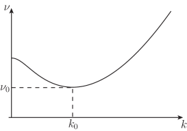
Figure 1: (a) Dispersion relation for linear hydroelastic waves. (b) Small-amplitude envelope solitary waves with speed $\nu=\nu_{0}+2(\nu_{0}f(k_{0}))^{-1}\mu^{2}\nu_{\mathrm{NLS}}$ (where $\nu_{\mathrm{NLS}}<0$) predicted by nonlinear Schrödinger theory.

Bifurcations of nonlinear solitary waves are expected whenever the linear group and phase speeds are equal, so that $\nu^{\prime}(k)=0$ (see Dias and Kharif [2, §3]). We therefore expect the existence of small-amplitude solitary waves with speed near $\nu_{0}$; the waves bifurcate from a linear periodic wave train with frequency $k_{0}\nu_{0}$ (see Figure 1(b)). The appropriate model equation for this type of solution is the cubic nonlinear Schrödinger equation

$$2\mathrm{i}A_{T}-\tfrac{1}{4}g^{\prime\prime}(k_{0})A_{XX}+\tfrac{3}{2}\left(\tfrac{1}{2}A_{3}+A_{4}\right)|A|^{2}A=0,$$ (5)

in which

$$\eta(x,t)=\tfrac{1}{2}\mu(A(X,T)\mathrm{e}^{\mathrm{i}k_{0}(x+\nu_{0}t)}+\mathrm{c.c.})+O(\mu^{2}),\qquad X=\mu(x+\nu_{0}t),\ T=2k_{0}(v_{0}f(k_{0}))^{-1}\mu^{2}t$$

and the abbreviation ‘c.c.’ denotes the complex conjugate of the preceding quantity; the values of the constants $A_{3}$ and $A_{4}$ are $A_{3}=-\tfrac{1}{3}g(2k_{0})^{-1}(A_{3}^{1})^{2}-\tfrac{2}{3}g(0)^{-1}(A_{3}^{2})^{2}$ and $A_{4}=A_{4}^{1}-\nu_{0}^{2}A_{4}^{2}$, where

$$A_{3}^{1}=\nu_{0}^{2}f(2k_{0})f(k_{0})+\tfrac{1}{2}\nu_{0}^{2}f(k_{0})^{2}-\tfrac{3}{2}\nu_{0}^{2}k_{0}^{2},\qquad A_{3}^{2}=\nu_{0}^{2}f(k_{0})+\tfrac{1}{2}\nu_{0}^{2}f(k_{0})^{2}-\tfrac{1}{2}\nu_{0}^{2}k_{0}^{2},$$

$$A_{4}^{1}=-\tfrac{5}{12}\gamma_{0}k_{0}^{6},\qquad A_{4}^{2}=\tfrac{1}{6}f(k_{0})^{2}(f(2k_{0})+2)-\tfrac{1}{2}k_{0}^{2}f(k_{0})$$

(see Milewski and Wang [6, §2] for a derivation of equation (5) in the present context). Note that $k_{0}>0$; the case $k_{0}=0$, which is associated with the Korteweg-de Vries scaling limit, does not arise here.

At this level of approximation, a solution to equation (5) of the form $A(X,T)=\mathrm{e}^{\mathrm{i}\nu_{\mathrm{NLS}}T}\zeta(X)$ with $\zeta(X)\rightarrow 0$ as $X\rightarrow\pm\infty$, so that $\zeta$ is a homoclinic solution of the ordinary differential equation

$$-\tfrac{1}{4}g^{\prime\prime}(k_{0})\zeta_{xx}-2\nu_{\mathrm{NLS}}\zeta+\tfrac{3}{2}\left(\tfrac{1}{2}A_{3}+A_{4}\right)|\zeta|^{2}\zeta=0$$ (6)

with $\nu_{\mathrm{NLS}}=-\tfrac{9}{8}\alpha_{\mathrm{NLS}}^{2}\,g^{\prime\prime}(k_{0})^{-1}\left(\tfrac{1}{2}A_{3}+A_{4}\right)^{2}$ and $\alpha_{\mathrm{NLS}}=2(\nu_{0}f(k_{0}))^{-1}$, corresponds to a solitary wave with speed $\nu=\nu_{0}+2(\nu_{0}f(k_{0}))^{-1}\mu^{2}\nu_{\mathrm{NLS}}$.

Proposition 1.2

Suppose that $\tfrac{1}{2}A_{3}+A_{4}<0$. The set of complex-valued homoclinic solutions to the ordinary differential equation (6) is $D_{\mathrm{NLS}}=\{\mathrm{e}^{\mathrm{i}\omega}\zeta_{\mathrm{NLS}}(\cdot+y)\colon\omega\in[0,2\pi),y\in{\mathbb{R}}\}$, where

$$\zeta_{\mathrm{NLS}}(x)=\alpha_{\mathrm{NLS}}\left(-3g^{\prime\prime}(k_{0})^{-1}\left(\tfrac{1}{2}A_{3}+A_{4}\right)\right)^{\frac{1}{2}}\operatorname{sech}\left(-3\alpha_{\mathrm{NLS}}\,g^{\prime\prime}(k_{0})^{-1}\left(\tfrac{1}{2}A_{3}+A_{4}\right)x\right).$$

Remark 2

Since $A_{3}<0$ and $\lim_{k_{0}\rightarrow 0}A_{4}=-\frac{1}{2}$, so that $A_{4}<0$ for sufficiently small values of $k_{0}$, we find that $\tfrac{1}{2}A_{3}+A_{4}<0$ for sufficiently small values of $k_{0}$, or equivalently for sufficiently large values of $\gamma$ (corresponding to sufficiently shallow water in physical variables). Numerics indicate that $\tfrac{1}{2}A_{3}+A_{4}<0$ for $k_{0}<177.33$, or equivalently $\gamma>3.37\times 10^{-10}$.

Our second theorem confirms the heuristic argument given above.

Theorem 1.2

Suppose that $\frac{1}{2}A_{3}+A_{4}<0$. The set $D_{\mu}$ of minimisers of ${\mathcal{E}}$ over $S_{\mu}$ satisfies

$$\sup_{(\eta,\Phi)\in D_{\mu}}\inf_{\omega\in[0,2\pi],x\in{\mathbb{R}}}\|\zeta_{\eta}-e^{\mathrm{i}\omega}\zeta_{\mathrm{NLS}}(\cdot+x)\|_{1}\rightarrow 0$$

as $\mu\downarrow 0$, where we write $\eta_{1}^{+}(x)=\tfrac{1}{2}\mu\zeta_{\eta}(\mu x)\mathrm{e}^{\mathrm{i}k_{0}x}$ and $\eta_{1}^{+}={\mathcal{F}}^{-1}[\chi_{[k_{0}-\delta_{0},k_{0}+\delta_{0}]}\hat{\eta}]$ with $\delta_{0}\in(0,\tfrac{1}{3}k_{0})$. Furthermore, the speed $\nu_{\mu}$ of the corresponding solitary wave satisfies $\nu_{\mu}=\nu_{0}+2(\nu_{0}f(k_{0}))^{-1}\nu_{\mathrm{NLS}}\mu^{2}+o(\mu^{2})$ uniformly over $(\eta,\Phi)\in D_{\mu}$.

2 The constrained minimisation problem

We tackle the constrained minimisation problem in two steps. (i) Fix $\eta\neq 0$ and minimise ${\mathcal{E}}(\eta,\cdot)$ over $T_{\mu}=\{\Phi\in H^{1/2}_{\star}({\mathbb{R}}):{\mathcal{I}}(\eta,\Phi)=2\mu\}$. This problem (of minimising a quadratic functional over a linear manifold) admits a unique global minimiser $\Phi_{\eta}$. (ii) Minimise ${\mathcal{J}}_{\mu}(\eta):={\mathcal{E}}(\eta,\Phi_{\eta})$ over $\eta\in U\setminus\{0\}$. Because $\Phi_{\eta}$ minimises ${\mathcal{E}}(\eta,\cdot)$ over $T_{\mu}$ there exists a Lagrange multiplier $\nu_{\eta}$ such that $G(\eta)\Phi_{\eta}=\nu_{\eta}\eta_{x}$, and straightforward calculations show that $\Phi_{\eta}=\nu_{\eta}G(\eta)^{-1}\eta_{x}$, $\nu_{\eta}=\mu/{\mathcal{L}}(\eta)$ and

$${\mathcal{J}}_{\mu}(\eta)={\mathcal{K}}(\eta)+\frac{\mu^{2}}{{\mathcal{L}}(\eta)},$$

where

$${\mathcal{K}}(\eta)=\frac{1}{2}\int_{-\infty}^{\infty}\left(\eta^{2}+\frac{\gamma\eta_{xx}^{2}}{(1+\eta_{x}^{2})^{5/2}}\right)\,\mathrm{d}x,\qquad{\mathcal{L}}(\eta)=\frac{1}{2}\int_{-\infty}^{\infty}\eta_{x}G(\eta)^{-1}\eta_{x}\,\mathrm{d}x.$$

This computation also shows that the dimensionless speed of the solitary wave corresponding to a constrained minimiser of ${\mathcal{E}}$ over $S_{\mu}$ is $\mu/{\mathcal{L}}(\eta)$.

A similar minimisation problem arises in the study of irrotational solitary water waves with weak surface tension (see Groves and Wahlén [3], taking $\omega=0$ and $\beta<\beta_{\mathrm{c}}$); in that case ${\mathcal{K}}(\eta)$ is replaced by $\tilde{\mathcal{K}}(\eta)=\int_{-\infty}^{\infty}\big{(}\tfrac{1}{2}\eta^{2}+\beta((1+\eta_{x}^{2})^{1/2}-1)\big{)}\,\mathrm{d}x$. In this note we describe the modifications necessary to apply the theory of Groves and Wahlén to the hydroelastic problem. The presence of the second-order derivative necessitates on the one hand non-trivial modifications because the $L^{2}({\mathbb{R}})$-gradient ${\mathcal{K}}^{\prime}(\eta)$ is not defined on the whole of $U$, but leads on the other hand to a more satisfactory final result (compare Theorem 1.1 with Theorem 1.5 of Groves & Wahlén).

Lemmata 2.1 and 2.2, in which we write $W^{s}:=W\cap H^{s}({\mathbb{R}})$, state some basic properties of the functionals ${\mathcal{K}}$ and ${\mathcal{L}}$ (see Groves and Wahlén [3] for the proof of the latter), while Proposition 2.1 is a useful ‘weak-strong’ argument. Note that the ‘linear’ estimates for ${\mathcal{K}}_{\mathrm{nl}}(\eta)$ and ${\mathcal{L}}_{\mathrm{nl}}(\eta)$ are used only to bound the $W^{1,\infty}({\mathbb{R}})$ norm of a minimising sequence for ${\mathcal{J}}$ over $U\setminus\{0\}$ away from zero (see the discussion at the beginning of Section 3).

Lemma 2.1

1. The functional ${\mathcal{K}}:H^{2}({\mathbb{R}})\rightarrow{\mathbb{R}}$ is analytic and satisfies ${\mathcal{K}}(0)=0$.

2. There exists a constant $D>0$ such that ${\mathcal{K}}(\eta)\geq D^{-1}\|\eta\|_{2}^{2}$ for all $\eta\in U$.

3. The $L^{2}({\mathbb{R}})$-gradient ${\mathcal{K}}^{\prime}(\eta)$ exists for each $\eta\in H^{4}({\mathbb{R}})$ and is given by the formula

   $${\mathcal{K}}^{\prime}(\eta)=\eta+\gamma\left[\frac{\eta_{xx}}{(1+\eta_{x}^{2})^{5/2}}\right]_{xx}+\frac{5}{2}\gamma\left[\frac{\eta_{x}\eta_{xx}^{2}}{(1+\eta_{x}^{2})^{7/2}}\right]_{x}.$$

   This formula defines an analytic function ${\mathcal{K}}^{\prime}:H^{2}({\mathbb{R}})\rightarrow H^{-2}({\mathbb{R}})$ which satisfies ${\mathcal{K}}^{\prime}(0)=0$.

4. The estimates $|{\mathcal{K}}_{4}(\eta)|\lesssim\|\eta\|_{2}^{2}\|\eta\|_{1,\infty}^{2}$, $|{\mathcal{K}}_{\mathrm{r}}(\eta)|\lesssim\|\eta\|_{2}^{3}\|\eta\|_{1,\infty}^{2}$, $|{\mathcal{K}}_{\mathrm{nl}}(\eta)|\lesssim\|\eta\|_{1,\infty}$ hold for all $\eta\in U$, where ${\mathcal{K}}_{n}(\eta)=\frac{1}{n!}\mathrm{d}^{n}{\mathcal{K}}[0](\{\eta\}^{n})$, ${\mathcal{K}}_{\mathrm{r}}(\eta)=\sum_{n=5}^{\infty}{\mathcal{K}}_{n}(\eta)$ and ${\mathcal{K}}_{\mathrm{nl}}(\eta)={\mathcal{K}}(\eta)-{\mathcal{K}}_{2}(\eta)$.

5. The estimates

   $$\|{\mathcal{F}}^{-1}[(1-\chi_{S}(k))g(k)^{-1/2}{\mathcal{F}}[{\mathcal{K}}_{4}^{\prime}(\eta)]]\|_{0}\lesssim\|\eta\|_{2}(\|\eta\|_{1,\infty}+\|\eta_{xx}+k_{0}^{2}\eta\|_{0})^{2},$$

   $$\|{\mathcal{F}}^{-1}[(1-\chi_{S}(k))g(k)^{-1/2}{\mathcal{F}}[{\mathcal{K}}_{\mathrm{r}}^{\prime}(\eta)]]\|_{0},\ |\langle{\mathcal{K}}_{4}^{\prime}(\eta),\eta\rangle_{0}|,\ |\langle{\mathcal{K}}_{\mathrm{r}}^{\prime}(\eta),\eta\rangle_{0}|\lesssim\|\eta\|_{2}^{2}(\|\eta\|_{1,\infty}+\|\eta_{xx}+k_{0}^{2}\eta\|_{0})^{2}$$

   hold for all $\eta\in H^{2}({\mathbb{R}})$, where $S=[-k_{0}-\delta_{0},-k_{0}+\delta_{0}]\cup[k_{0}-\delta_{0},k_{0}+\delta_{0}]$ and $\delta_{0}\in(0,\tfrac{1}{3}k_{0})$.

Proof. Assertions (i)–(iv) follow by straightforward estimates. Turning to (v), note that

$${\mathcal{K}}_{4}^{\prime}(\eta)=\tfrac{5}{2}\gamma\big{(}(\eta_{x}\eta_{xx}^{2})_{x}+(\eta_{x}^{2}\eta_{xx})_{xx}\big{)}=\tfrac{5}{2}\gamma\left(\big{(}\eta_{x}(\eta_{xx}+k_{0}^{2}\eta)^{2}-2k_{0}^{2}\eta_{x}\eta(\eta_{xx}+k_{0}^{2}\eta)+k_{0}^{4}\eta_{x}\eta^{2}\big{)}_{x}+\big{(}\eta_{x}^{2}\eta_{xx})_{xx}\right)$$

so that

$$\|{\mathcal{F}}^{-1}[(1-\chi_{S}(k))g(k)^{-1/2}{\mathcal{F}}[{\mathcal{K}}_{4}^{\prime}(\eta)]]\|_{0} \lesssim\|\eta_{x}(\eta_{xx}+k_{0}^{2}\eta)^{2}\|_{-1}+\|\eta_{x}\eta(\eta_{xx}+k_{0}^{2}\eta)\|_{0}+\|\eta_{x}\eta^{2}\|_{0}+\|\eta_{x}^{2}\eta_{xx}\|_{0}$$

$$\lesssim\|\eta_{x}(\eta_{xx}+k_{0}^{2}\eta)\|_{0}\|\eta_{xx}+k_{0}^{2}\eta\|_{0}+\|\eta\|_{2}\|\eta\|_{1,\infty}^{2}$$

$$\lesssim\|\eta\|_{2}(\|\eta\|_{1,\infty}+\|\eta_{xx}+k_{0}^{2}\eta\|_{0})^{2},$$

where we have used the inequalities $(1-\chi_{S}(k))g(k)^{-1/2}\lesssim(1+|k|^{2})^{-1}$ and $\|u_{1}u_{2}\|_{-1}\lesssim\|u_{1}\|_{0}\|u_{2}\|_{0}$ (see Hörmander [5, Theorem 8.3.1]); the remaining estimates are obtained in a similar fashion.∎

Lemma 2.2

1. Suppose $s>0$. The functional ${\mathcal{L}}:W^{s+3/2}\rightarrow{\mathbb{R}}$ is analytic and satisfies ${\mathcal{L}}(0)=0$.

2. The estimates $\|\eta\|_{1/2}^{2}\lesssim{\mathcal{L}}(\eta),{\mathcal{L}}_{2}(\eta)\lesssim\|\eta\|_{1/2}^{2}$, where ${\mathcal{L}}_{2}(\eta)=\frac{1}{2!}\mathrm{d}^{2}{\mathcal{L}}[0](\{\eta\}^{2})$, hold for all $\eta\in U$.

3. Suppose $s>0$. The $L^{2}({\mathbb{R}})$-gradient ${\mathcal{L}}^{\prime}(\eta)$ exists for each $\eta\in W^{s+3/2}$ and defines an analytic function ${\mathcal{L}}^{\prime}:W^{s+3/2}\rightarrow H^{s+1/2}({\mathbb{R}})$ which satisfies ${\mathcal{L}}^{\prime}(0)=0$.

4. Suppose that $\{M_{n}^{(1)}\}$, $\{M_{n}^{(2)}\}\subseteq{\mathbb{R}}$ and $\{\eta_{n}^{(1)}\}$, $\{\eta_{n}^{(2)}\}\subseteq U$ are sequences with $M_{n}^{(1)}$, $M_{n}^{(2)}\rightarrow\infty$, $M_{n}^{(1)}/M_{n}^{(2)}\rightarrow 0$, $\{\eta_{n}^{(1)}+\eta_{n}^{(2)}\}\subseteq U$ and $\mathrm{supp}\,\eta_{n}^{(1)}\subseteq(-2M_{n}^{(1)},2M_{n}^{(1)})$, $\mathrm{supp}\,\eta_{n}^{(2)}\subseteq{\mathbb{R}}\setminus(-M_{n}^{(2)},M_{n}^{(2)})$. The functional ${\mathcal{L}}$ has the ‘pseudolocal’ properties

   $${\mathcal{L}}(\eta_{n}^{(1)}+\eta_{n}^{(2)})-{\mathcal{L}}(\eta_{n}^{(1)})-{\mathcal{L}}(\eta_{n}^{(2)})\rightarrow 0,\qquad\|{\mathcal{L}}^{\prime}(\eta_{n}^{(1)}+\eta_{n}^{(2)})-{\mathcal{L}}^{\prime}(\eta_{n}^{(1)})-{\mathcal{L}}^{\prime}(\eta_{n}^{(2)})\|_{0}\rightarrow 0$$

   and $\langle{\mathcal{L}}^{\prime}(\eta_{n}^{(2)}),\phi\rangle_{0}\rightarrow 0$ for each $\phi\in C_{0}^{\infty}({\mathbb{R}})$.

5. The estimates

   $$|{\mathcal{L}}_{3}(\eta)|\lesssim\|\eta\|_{2}^{2}(\|\eta\|_{1,\infty}+\|\eta_{xx}+k_{0}^{2}\eta\|_{0}),\qquad|{\mathcal{L}}_{4}(\eta)|\lesssim\|\eta\|_{2}^{2}(\|\eta\|_{1,\infty}+\|\eta_{xx}+k_{0}^{2}\eta\|_{0})^{2},$$

   $$|{\mathcal{L}}_{\mathrm{r}}(\eta)|\lesssim\|\eta\|_{2}^{3}(\|\eta\|_{1,\infty}+\|\eta_{xx}+k_{0}^{2}\eta\|_{0})^{2},\qquad|{\mathcal{L}}_{\mathrm{nl}}(\eta)|\lesssim\|\eta\|_{1,\infty},$$

   where ${\mathcal{L}}_{n}(\eta)=\frac{1}{n!}\mathrm{d}^{n}{\mathcal{L}}[0](\{\eta\}^{n})$, ${\mathcal{L}}_{\mathrm{r}}(\eta)=\sum_{n=5}^{\infty}{\mathcal{L}}_{n}(\eta)$ and ${\mathcal{L}}_{\mathrm{nl}}(\eta)={\mathcal{L}}(\eta)-{\mathcal{L}}_{2}(\eta)$, and

   $$\|{\mathcal{L}}_{3}^{\prime}(\eta)\|_{0} \lesssim\|\eta\|_{2}(\|\eta\|_{1,\infty}+\|\eta_{xx}+k_{0}^{2}\eta\|_{0}+\|K^{0}\eta\|_{\infty}),$$

   $$\|{\mathcal{L}}_{4}^{\prime}(\eta)\|_{0} \lesssim\|\eta\|_{2}(\|\eta\|_{1,\infty}+\|\eta_{xx}+k_{0}^{2}\eta\|_{0}+\|K^{0}\eta\|_{\infty})^{2},$$

   $$\|{\mathcal{L}}_{\mathrm{r}}^{\prime}(\eta)\|_{0} \lesssim\|\eta\|_{2}^{2}(\|\eta\|_{1,\infty}+\|\eta_{xx}+k_{0}^{2}\eta\|_{0})^{2},$$

   where $K_{0}\eta:={\mathcal{F}}^{-1}[f(k)\hat{\eta}]$, hold for all $\eta\in U$.

Proposition 2.1

Suppose that $\{\eta_{n}\}\subseteq U$ and $\eta\in U$ have the properties that $\eta_{n}\rightharpoonup\eta$ in $H^{2}({\mathbb{R}})$ and $\eta_{n}\rightarrow\eta$ in $L^{2}({\mathbb{R}})$ (and hence in $H^{s}({\mathbb{R}})$ for all $s\in[0,2)$). The inequality ${\mathcal{K}}(\eta)\leq\lim_{n\rightarrow\infty}{\mathcal{K}}(\eta_{n})$ holds whenever $\{{\mathcal{K}}(\eta_{n})\}$ is convergent, and equality implies that $\eta_{n}\rightarrow\eta$ in $H^{2}({\mathbb{R}})$.

Proof. Note that $(1+\eta_{nx}^{2})^{-5/4}\eta_{nxx}\rightharpoonup(1+\eta_{x}^{2})^{-5/4}\eta_{xx}$ in $L^{2}({\mathbb{R}})$, and it follows from the weak lower semicontinuity of $\|\cdot\|_{0}^{2}$ (and $\eta_{n}\rightarrow\eta$ in $L^{2}({\mathbb{R}})$) that ${\mathcal{K}}(\eta)\leq\lim_{n\rightarrow\infty}{\mathcal{K}}(\eta_{n})$. Moreover, ${\mathcal{K}}(\eta_{n})\rightarrow{\mathcal{K}}(\eta)$ implies that $\|(1+\eta_{nx}^{2})^{-5/4}\eta_{nxx}\|_{0}\rightarrow\|(1+\eta_{x}^{2})^{-5/4}\eta_{xx}\|_{0}$, so that $(1+\eta_{nx}^{2})^{-5/4}\eta_{nxx}\rightarrow(1+\eta_{x}^{2})^{-5/4}\eta_{xx}$ in $L^{2}({\mathbb{R}})$ and hence $\eta_{nxx}\rightarrow\eta_{xx}$ in $L^{2}({\mathbb{R}})$.∎

Next we establish some basic properties of ${\mathcal{J}}_{\mu}$. The following proposition (cf. Groves and Wahlén [3, Appendix A.2]) shows in particular that $c_{\mu}:=\inf_{\eta\in U\setminus\{0\}}{\mathcal{J}}_{\mu}(\eta)<2\nu_{0}\mu$, while Lemma 2.3 shows that its critical points have additional regularity.

Proposition 2.2

The continuous mapping $\alpha\mapsto\nu_{0}{\mathcal{L}}(\eta^{\star}_{\alpha})$, where

$$\eta^{\star}_{\alpha}(x)=\alpha\zeta_{\mathrm{NLS}}(\alpha x)\cos k_{0}x-\tfrac{1}{2}\alpha^{2}g(2k_{0})^{-1}A_{3}^{1}\zeta_{\mathrm{NLS}}(\alpha x)^{2}\cos 2k_{0}x-\tfrac{1}{2}\alpha^{2}g(0)^{-1}A_{3}^{2}\zeta_{\mathrm{NLS}}(\alpha x)^{2},$$

is invertible, and its (continuous) inverse $\mu\mapsto\alpha(\mu)$ satisfies ${\mathcal{J}}_{\mu}(\eta^{\star}_{\alpha(\mu)})=2\nu_{0}\mu+c_{\mathrm{NLS}}\mu^{3}+o(\mu^{3})$, where $c_{\mathrm{NLS}}=-\frac{3}{4}\alpha_{\mathrm{NLS}}^{3}g^{\prime\prime}(k_{0})^{-1}(\frac{1}{2}A_{3}+A_{4})^{2}$.

Remark 3

Each $\eta\in U\setminus\{0\}$ satisfies

$${\mathcal{K}}_{2}(\eta)+\frac{\mu^{2}}{{\mathcal{L}}_{2}(\eta)}={\mathcal{K}}_{2}(\eta)-\nu_{0}^{2}{\mathcal{L}}_{2}(\eta)+\frac{(\mu-\nu_{0}{\mathcal{L}}_{2}(\eta))^{2}}{{\mathcal{L}}_{2}(\eta)}+2\nu_{0}\mu\geq\frac{1}{2}\int_{-\infty}^{\infty}g(k)|\hat{\eta}|^{2}\,\mathrm{d}k+2\nu_{0}\mu\geq 2\nu_{0}\mu.$$

Lemma 2.3

Any critical point $\eta\in U\setminus\{0\}$ of ${\mathcal{J}}_{\mu}$ belongs to $H^{4}({\mathbb{R}})$.

Proof. Write $u=(1+\eta_{x}^{2})^{-5/2}\eta_{xx}$, so that $\eta_{x}(1+\eta_{x}^{2})^{3/2}u^{2}\in L^{1}({\mathbb{R}})\subseteq H^{-3/4}({\mathbb{R}})$, and observe that

$$\gamma u_{xx}=\frac{\mu}{{\mathcal{L}}(\eta)^{2}}{\mathcal{L}}^{\prime}(\eta)-\eta-\tfrac{5}{2}\gamma\big{(}\eta_{x}(1+\eta_{x}^{2})^{3/2}u^{2}\big{)}_{x}$$ (7)

in the sense of distributions since $\eta$ is a critical point of ${\mathcal{J}}_{\mu}$. It follows from (7) and the fact that ${\mathcal{L}}^{\prime}(\eta)\in L^{2}({\mathbb{R}})$ that $\gamma u_{xx}\in H^{-7/4}({\mathbb{R}})$, that is $u\in H^{1/4}({\mathbb{R}})$. We conclude that $u^{2}\in L^{2}({\mathbb{R}})$ (see Hörmander [5, Theorem 8.3.1]), so that $\eta_{x}(1+\eta_{x}^{2})^{3/2}u^{2}\in L^{2}({\mathbb{R}})$ and hence $\gamma u_{xx}\in H^{-1}({\mathbb{R}})$, that is $u\in H^{1}({\mathbb{R}})$.

Observing that $\eta_{x}(1+\eta_{x}^{2})^{3/2}u^{2}\in H^{1}({\mathbb{R}})$, one finds from (7) that $\gamma u_{xx}\in L^{2}({\mathbb{R}})$, $u\in H^{2}({\mathbb{R}})$ and finally $\eta\in H^{4}({\mathbb{R}})$ (because $\eta_{xx}=(1+\eta_{x}^{2})^{5/2}u$).∎

Theorem 1.1 is a consequence of the following result (cf. Groves & Wahlén [3, Theorem 5.2]).

Theorem 2.4

Suppose that $\frac{1}{2}A_{3}+A_{4}<0$.

1. The set $B_{\mu}$ of minimisers of ${\mathcal{J}}_{\mu}$ over $U\setminus\{0\}$ is nonempty and lies in $H^{4}({\mathbb{R}})$. Moreover, each $\eta\in B_{\mu}$ satisfies $\|\eta\|_{2}^{2}\leq 2D\nu_{0}\mu$.

2. Suppose that $\{\eta_{n}\}$ is a minimising sequence for ${\mathcal{J}}_{\mu}$ over $U\setminus\{0\}$. There exists a sequence $\{x_{n}\}\subseteq{\mathbb{R}}$ with the property that there exists a subsequence of $\{\eta_{n}(x_{n}+\cdot)\}$ which converges in $H^{2}({\mathbb{R}})$ to a function $\eta\in B_{\mu}$.

Any function $\eta\in U$ with ${\mathcal{J}}_{\mu}(\eta)<2\nu_{0}\mu$ satisfies $\|\eta\|_{2}^{2}<2D\nu_{0}\mu$, ${\mathcal{L}}(\eta)>\mu/(2\nu_{0})$ and ${\mathcal{L}}_{2}(\eta)\gtrsim\mu$ (see Lemmata 2.1(ii) and 2.2(ii)). These properties are enjoyed in particular by a minimising sequence $\{\eta_{n}\}$ for ${\mathcal{J}}_{\mu}$ over $U\setminus\{0\}$, which also satisfies ${\mathcal{M}}_{\mu}(\eta_{n})\lesssim-\mu^{3}$, where ${\mathcal{M}}_{\mu}(\eta)={\mathcal{J}}_{\mu}(\eta)-{\mathcal{K}}_{2}(\eta)-\mu^{2}/{\mathcal{L}}_{2}(\eta)$ (Proposition 2.2), and hence $\|\eta_{n}\|_{1,\infty}\gtrsim\mu^{3}$ (because $|{\mathcal{K}}_{\mathrm{nl}}(\eta_{n})|$, $|{\mathcal{L}}_{\mathrm{nl}}(\eta_{n})|\lesssim\|\eta_{n}\|_{1,\infty}$). Furthermore, we may without loss of generality assume that $\{\eta_{n}\}$ is a Palais-Smale sequence, so that $\mathrm{d}{\mathcal{J}}_{\mu}[\eta_{n}]\rightarrow 0$ in $(H^{2}({\mathbb{R}}))^{\ast}$, and the calculation

$$\|{\mathcal{J}}^{\prime}(\eta_{n})\|_{-2}=\sup\{\langle{\mathcal{J}}^{\prime}(\eta_{n}),\phi\rangle_{0}:\phi\in H^{2}({\mathbb{R}}),\|\phi\|_{2}=1\}=\|\mathrm{d}{\mathcal{J}}_{\mu}[\eta_{n}]\|_{(H^{2}({\mathbb{R}}))^{\ast}}$$

shows that ${\mathcal{J}}^{\prime}(\eta_{n})\rightarrow 0$ in $H^{-2}({\mathbb{R}})$. Theorem 2.4 is proved by applying the concentration-compactness principle to the sequence $\{\eta_{nx}^{2}+\eta_{n}^{2}\}\subseteq L^{1}({\mathbb{R}})$ under the additional hypothesis that $c_{\mu}$ is a strictly sub-additive function of $\mu$, which is verified in Section 3 below.

‘Vanishing’ is excluded since it implies that $\|\eta_{n}\|_{1,\infty}\rightarrow 0$, which contradicts the estimate $\|\eta_{n}\|_{1,\infty}\gtrsim\mu^{3}$ (see above).

‘Dichotomy’ leads to the existence of sequences $\{\eta_{n}^{(1)}\}$, $\{\eta_{n}^{(2)}\}$ of the kind described in Lemma 2.2(iv) with $\lim_{n\rightarrow\infty}\|\eta_{n}-\eta_{n}^{(1)}-\eta_{n}^{(2)}\|_{2}=0$ (up to subsequences and translations), so that in particular

$$\lim_{n\rightarrow\infty}{\mathcal{J}}_{\mu}(\eta_{n})=\lim_{n\rightarrow\infty}{\mathcal{J}}_{\mu^{(1)}}(\eta_{n}^{(1)})+\lim_{n\rightarrow\infty}{\mathcal{J}}_{\mu^{(2)}}(\eta_{n}^{(2)}),$$

where $\mu^{(j)}\ =\ \mu\lim_{n\rightarrow\infty}{\mathcal{L}}(\eta_{n}^{(j)})/\lim_{n\rightarrow\infty}\vphantom{{\mathcal{L}}^{2}}{\mathcal{L}}(\eta_{n})$ (so that $\mu^{(1)}+\mu^{(2)}=\mu$). We thus obtain the contradiction

$$c_{\mu}<c_{\mu^{(1)}}+c_{\mu^{(2)}}\leq\lim_{n\rightarrow\infty}{\mathcal{J}}_{\mu^{(1)}}(\eta_{n}^{(1)})+\lim_{n\rightarrow\infty}{\mathcal{J}}_{\mu^{(2)}}(\eta_{n}^{(2)})=\lim_{n\rightarrow\infty}{\mathcal{J}}_{\mu}(\eta_{n})=c_{\mu},$$

which excludes ‘dichotomy’.

‘Concentration’ implies the existence of $\eta\in U$ with $\eta_{n}\rightharpoonup\eta$ in $H^{2}({\mathbb{R}})$ and $\eta_{n}\rightarrow\eta$ in $L^{2}({\mathbb{R}})$ (up to subsequences and translations). Since ${\mathcal{K}}(\eta_{n})\leq{\mathcal{J}}_{\mu}(\eta_{n})<2\nu_{0}\mu$ the sequence $\{{\mathcal{K}}(\eta_{n})\}$ is bounded and hence admits a convergent subsequence (still denoted by $\{{\mathcal{K}}(\eta_{n})\}$) which satisfies ${\mathcal{K}}(\eta)\leq\lim_{n\rightarrow\infty}{\mathcal{K}}(\eta_{n})$ (Proposition 2.1). Lemma 2.2(i) asserts that ${\mathcal{L}}(\eta_{n})\rightarrow{\mathcal{L}}(\eta)$, so that ${\mathcal{J}}_{\mu}(\eta)\leq\lim_{n\rightarrow\infty}{\mathcal{J}}(\eta_{n})=c_{\mu}$, which therefore holds with equality; it follows that ${\mathcal{K}}(\eta_{n})\rightarrow{\mathcal{K}}(\eta)$ and hence $\eta_{n}\rightarrow\eta$ in $H^{2}({\mathbb{R}})$ (Proposition 2.1), so that $\eta$ minimises ${\mathcal{J}}_{\mu}$ over $U\setminus\{0\}$.

3 Strict sub-additivity

We begin by deriving sharper estimates for a ‘near minimiser’ of ${\mathcal{J}}_{\mu}$ over $U\setminus\{0\}$, that is a function $\tilde{\eta}\in U\setminus\{0\}$ with $\|{\mathcal{J}}_{\mu}^{\prime}(\tilde{\eta})\|_{-2}\leq\mu^{N}$ for some $N\in{\mathbb{N}}$ and ${\mathcal{J}}_{\mu}(\tilde{\eta})<2\nu_{0}\mu$ (and hence $\|\tilde{\eta}\|_{2}\lesssim\mu^{1/2}$, ${\mathcal{L}}(\tilde{\eta})$, ${\mathcal{L}}_{2}(\tilde{\eta})\geq\mu$); these estimates apply in particular to a minimising sequence $\{\eta_{n}\}$ for ${\mathcal{J}}_{\mu}$ over $U\setminus\{0\}$.

We write the equation ${\mathcal{J}}^{\prime}_{\mu}(\eta)={\mathcal{K}}^{\prime}(\eta)-(\mu/{\mathcal{L}}(\eta))^{2}{\mathcal{L}}^{\prime}(\eta)$ for $\eta\in U$ in the form

$$g(k)\hat{\eta}={\mathcal{F}}\left[{\mathcal{J}}^{\prime}_{\mu}(\eta)-{\mathcal{K}}_{\mathrm{nl}}^{\prime}(\eta)+\left(\frac{\mu}{{\mathcal{L}}(\eta)}+\nu_{0}\right)\!\!\!\left(\frac{\mu}{{\mathcal{L}}(\eta)}-\nu_{0}\right){\mathcal{L}}_{2}^{\prime}(\eta)+\left(\frac{\mu}{{\mathcal{L}}(\eta)}\right)^{2}{\mathcal{L}}_{\mathrm{nl}}^{\prime}(\eta)\right]$$

and decompose it into two coupled equations by defining $\eta_{2}\in H^{2}({\mathbb{R}})$ by the formula

$$\eta_{2}={\mathcal{F}}^{-1}\left[\frac{1-\chi_{S}(k)}{g(k)}{\mathcal{F}}\left[{\mathcal{J}}^{\prime}_{\mu}(\eta)-{\mathcal{K}}_{\mathrm{nl}}^{\prime}(\eta)+\left(\frac{\mu}{{\mathcal{L}}(\eta)}+\nu_{0}\right)\!\!\!\left(\frac{\mu}{{\mathcal{L}}(\eta)}-\nu_{0}\right){\mathcal{L}}_{2}^{\prime}(\eta)+\left(\frac{\mu}{{\mathcal{L}}(\eta)}\right)^{2}{\mathcal{L}}_{\mathrm{nl}}^{\prime}(\eta)\right]\right]$$

(recall that $(1-\chi_{S}(k))g(k)^{-1/2}\lesssim(1+|k|^{2})^{-1}$) and $\eta_{1}\in H^{2}({\mathbb{R}})$ by $\eta_{1}=\eta-\eta_{2}$, so that $\mathrm{supp}\,\hat{\eta}_{1}\in S$ and $\chi_{S}{\mathcal{L}}_{3}^{\prime}(\eta_{1})=0$ (see Groves and Wahlén [3, Proposition 4.15]). We accordingly write these equations as

$$g(k)\hat{\eta}_{1}=\chi_{S}(k){\mathcal{F}}[{\mathcal{R}}(\eta)-{\mathcal{K}}_{\mathrm{nl}}^{\prime}(\eta)],\qquad\eta_{3}:=\eta_{2}+H(\eta)={\mathcal{F}}^{-1}\left[\frac{1-\chi_{S}(k)}{g(k)}{\mathcal{F}}[{\mathcal{R}}(\eta)-{\mathcal{K}}_{\mathrm{nl}}^{\prime}(\eta)]\right],$$

where

$$H(\eta):={\mathcal{F}}^{-1}\left[\frac{1}{g(k)}{\mathcal{F}}\left[-\Big{(}\frac{\mu}{{\mathcal{L}}(\eta)}\Big{)}^{2}{\mathcal{L}}_{3}^{\prime}(\eta_{1})\right]\right],$$

$${\mathcal{R}}(\eta):={\mathcal{J}}^{\prime}_{\mu}(\eta)+\left(\frac{\mu}{{\mathcal{L}}(\eta)}+\nu_{0}\right)\!\!\!\left(\frac{\mu}{{\mathcal{L}}(\eta)}-\nu_{0}\right){\mathcal{L}}_{2}^{\prime}(\eta)+\left(\frac{\mu}{{\mathcal{L}}(\eta)}\right)^{2}({\mathcal{L}}_{\mathrm{nl}}^{\prime}(\eta)-{\mathcal{L}}_{3}^{\prime}(\eta_{1})).$$

The next step is to study $\eta_{1}$ using the scaled norm

$$|{\mskip-2.0mu}|{\mskip-2.0mu}|\eta_{1}|{\mskip-2.0mu}|{\mskip-2.0mu}|_{\alpha}:=\left(\int_{-\infty}^{\infty}(1+\mu^{-4\alpha}(|k|-k_{0})^{4})|\hat{\eta}_{1}(k)|^{2}\,\mathrm{d}k\right)^{1/2}$$

for $H^{2}({\mathbb{R}})$; we choose $\alpha>0$ as large as possible so that $|{\mskip-2.0mu}|{\mskip-2.0mu}|\tilde{\eta}_{1}|{\mskip-2.0mu}|{\mskip-2.0mu}|_{\alpha}\lesssim\mu^{1/2}$.

Lemma 3.1

Each near minimiser $\tilde{\eta}$ of ${\mathcal{J}}_{\mu}$ over $U\setminus\{0\}$ satisfies $\|H(\tilde{\eta})\|_{2}\lesssim\mu^{1/2+\alpha/2}|{\mskip-2.0mu}|{\mskip-2.0mu}|\tilde{\eta}_{1}|{\mskip-2.0mu}|{\mskip-2.0mu}|_{\alpha}$,$\|{\mathcal{R}}(\tilde{\eta})\|_{-2}\lesssim\mu^{1/2+\alpha}|{\mskip-2.0mu}|{\mskip-2.0mu}|\tilde{\eta}_{1}|{\mskip-2.0mu}|{\mskip-2.0mu}|_{\alpha}^{2}+\mu^{N}$ and $\|{\mathcal{F}}^{-1}[(1-\chi_{S}(k))g(k)^{-1/2}{\mathcal{F}}[{\mathcal{K}}_{\mathrm{nl}}^{\prime}(\tilde{\eta})]]\|_{0}\lesssim\mu^{1/2+\alpha}|{\mskip-2.0mu}|{\mskip-2.0mu}|\tilde{\eta}_{1}|{\mskip-2.0mu}|{\mskip-2.0mu}|_{\alpha}^{2}+\mu\|\tilde{\eta}_{3}\|_{2}$.

Proof. The results for $H(\tilde{\eta})$ and ${\mathcal{R}}(\tilde{\eta})$ were derived by Groves & Wahlén [3, §4.3.1], while that for ${\mathcal{K}}_{\mathrm{nl}}^{\prime}(\tilde{\eta})$ follows from Lemma 2.1(v) and the estimates $\|\eta_{1}\|_{1,\infty}\lesssim\mu^{\alpha/2}|{\mskip-2.0mu}|{\mskip-2.0mu}|\eta_{1}|{\mskip-2.0mu}|{\mskip-2.0mu}|_{\alpha}$ and $\|\eta_{1xx}+k_{0}^{2}\eta_{1}\|_{0}\leq c\mu^{\alpha}|{\mskip-2.0mu}|{\mskip-2.0mu}|\eta_{1}|{\mskip-2.0mu}|{\mskip-2.0mu}|_{\alpha}$ (Groves and Wahlén [3, Proposition 4.1]).∎

Square integrating the equation $g(k)\hat{\eta}_{1}=\chi(k){\mathcal{F}}[{\mathcal{R}}(\eta)-{\mathcal{K}}_{\mathrm{nl}}^{\prime}(\eta)]$, multiplying by $\mu^{-4\alpha}$ and adding $\|\tilde{\eta}_{1}\|_{0}^{2}\lesssim\mu$ yields $|{\mskip-2.0mu}|{\mskip-2.0mu}|\tilde{\eta}_{1}|{\mskip-2.0mu}|{\mskip-2.0mu}|_{\alpha}^{2}\lesssim\mu^{1-2\alpha}|{\mskip-2.0mu}|{\mskip-2.0mu}|\tilde{\eta}_{1}|{\mskip-2.0mu}|{\mskip-2.0mu}|_{\alpha}^{4}+\mu$, which implies that $|{\mskip-2.0mu}|{\mskip-2.0mu}|\tilde{\eta}_{1}|{\mskip-2.0mu}|{\mskip-2.0mu}|_{\alpha}^{2}\lesssim\mu$ for each $\alpha<1$; it follows that $\|\tilde{\eta}_{3}\|_{2}^{2}\lesssim\mu^{3+2\alpha}$ and $\|H(\tilde{\eta})\|_{2}^{2}\lesssim\mu^{2+\alpha}$ for each $\alpha<1$. These estimates are used to establish the following proposition (see Groves & Wahlén [3, §4.3.2]).

Proposition 3.1

Suppose that $\tilde{\eta}$ is a near minimiser of ${\mathcal{J}}_{\mu}$ over $U\setminus\{0\}$. The estimates

$${\mathcal{M}}_{a^{2}\mu}(a\tilde{\eta}) =-a^{3}\nu_{0}^{2}{\mathcal{L}}_{3}(\tilde{\eta})-a^{4}\nu_{0}^{2}{\mathcal{L}}_{4}(\tilde{\eta})+a^{3}o(\mu^{3}),$$

$$\langle{\mathcal{M}}_{a^{2}\mu}^{\prime}(a\tilde{\eta}),a\tilde{\eta}\rangle_{0}+4a^{2}\mu\tilde{{\mathcal{M}}}_{a^{2}\mu}(a\tilde{\eta}) =-3a^{3}\nu_{0}^{2}{\mathcal{L}}_{3}(\tilde{\eta})-4a^{4}\nu_{0}^{2}{\mathcal{L}}_{4}(\tilde{\eta})+a^{3}o(\mu^{3}),$$

where $\tilde{\mathcal{M}}_{\mu}(\eta)=\mu/{\mathcal{L}}(\eta)-\mu/{\mathcal{L}}_{2}(\eta)$, hold uniformly over $a\in[1,2]$.

Lemma 3.2

Each near minimiser $\tilde{\eta}$ of ${\mathcal{J}}_{\mu}$ over $U\setminus\{0\}$ satisfies the estimate

$${\mathcal{K}}_{4}(\tilde{\eta})=A_{4}^{1}\int_{-\infty}^{\infty}\tilde{\eta}_{1}^{4}\,\mathrm{d}x+o(\mu^{3}).$$

Proof. We expand the right-hand side of the formula

$${\mathcal{K}}_{4}(\tilde{\eta})=-\frac{5}{4}\gamma\int_{-\infty}^{\infty}(\partial_{x}(\tilde{\eta}_{1}+H(\tilde{\eta})+\tilde{\eta}_{3}))^{2}\partial_{x}^{2}((\tilde{\eta}_{1}+H(\tilde{\eta})+\tilde{\eta}_{3}))^{2}\,\mathrm{d}x;$$

terms with zero, one or two occurrences of $\tilde{\eta}_{1}$ are $O((\|\tilde{\eta}_{1}\|_{2}+\|H(\tilde{\eta})\|_{2}+\|\tilde{\eta}_{3}\|_{2})^{2}(\|H(\tilde{\eta})\|_{2}+\|\tilde{\eta}_{3}\|_{2})^{2})$and hence $O(\mu\mu^{2+\alpha})=o(\mu^{3}),$ while terms with three occurrences of $\tilde{\eta}_{1}$ are estimated by$O((\|\tilde{\eta}_{1}\|_{1,\infty}+\|\tilde{\eta}_{1xx}+k_{0}^{2}\tilde{\eta}_{1}\|_{0})\|\tilde{\eta}_{1}\|_{2}^{2}(\|H(\tilde{\eta})\|_{2}+\|\tilde{\eta}_{3}\|_{2})^{2})=O(\mu^{2+\alpha}|{\mskip-2.0mu}|{\mskip-2.0mu}|\tilde{\eta}_{1}|{\mskip-2.0mu}|{\mskip-2.0mu}|)=O(\mu^{5/2+\alpha})=o(\mu^{3})$, so that ${\mathcal{K}}_{4}(\tilde{\eta})=-\frac{5}{4}\gamma\int_{-\infty}^{\infty}\tilde{\eta}_{1x}^{2}\tilde{\eta}_{1xx}^{2}+o(\mu^{3})$.

Writing $\tilde{\eta}_{1}=\tilde{\eta}_{1}^{+}+\tilde{\eta}_{1}^{-}$, where $\tilde{\eta}_{1}^{+}={\mathcal{F}}^{-1}[\chi_{[0,\infty)}{\mathcal{F}}[\tilde{\eta}_{1}]]$, $\tilde{\eta}_{1}^{-}={\mathcal{F}}^{-1}[\chi_{(-\infty,0]}{\mathcal{F}}[\tilde{\eta}_{1}]]$, we find that

$$\|(\mathrm{i}k\mp\mathrm{i}k_{0})\tilde{\eta}_{1}^{\pm}\|_{s}^{2}=\|(|k|-k_{0}){\mathcal{F}}[\tilde{\eta}_{1}]\|_{0}^{2}\leq\frac{1}{2}\int_{-\infty}^{\infty}(\mu^{2\alpha}+\mu^{-2\alpha}(|k|-k_{0})^{4})|{\mathcal{F}}[\tilde{\eta}_{1}]|^{2}\,\mathrm{d}k\lesssim\mu^{2\alpha}|{\mskip-2.0mu}|{\mskip-2.0mu}|\tilde{\eta}_{1}|{\mskip-2.0mu}|{\mskip-2.0mu}|^{2}\lesssim\mu^{1+2\alpha}$$

so that $(\tilde{\eta}_{1}^{\pm})_{x}=\pm\mathrm{i}k_{0}+O(\mu^{1+2\alpha})$ in $H^{s}({\mathbb{R}})$ for each $s\geq 0$. Using this estimate, one concludes that

$$\int_{-\infty}^{\infty}\tilde{\eta}_{1x}^{2}\tilde{\eta}_{1xx}^{2}\,\mathrm{d}x =\int_{-\infty}^{\infty}\left((\tilde{\eta}_{1x}^{+})^{2}(\tilde{\eta}_{1xx}^{-})^{2}+(\tilde{\eta}_{1x}^{-})^{2}(\tilde{\eta}_{1xx}^{+})^{2}+4\tilde{\eta}_{1x}\tilde{\eta}_{1x}^{-}\tilde{\eta}_{1xx}^{+}\tilde{\eta}_{1xx}^{-}\right)\,\mathrm{d}x$$

$$=2k_{0}^{6}\int_{-\infty}^{\infty}(\tilde{\eta}_{1}^{+})^{2}(\tilde{\eta}_{1}^{-})^{2}\,\mathrm{d}x+o(\mu)$$

$$=\frac{1}{3}k_{0}^{2}\int_{-\infty}^{\infty}\tilde{\eta}_{1}^{4}\,\mathrm{d}x+o(\mu).\qed$$

The corresponding estimates for ${\mathcal{L}}_{3}(\tilde{\eta})$ and ${\mathcal{L}}_{4}(\tilde{\eta})$ are derived similarly by Groves and Wahlén [3, §4.3.2].

Lemma 3.3

Each near minimiser $\tilde{\eta}$ of ${\mathcal{J}}_{\mu}$ over $U\setminus\{0\}$ satisfies the estimates

$$-\nu_{0}^{2}{\mathcal{L}}_{3}(\tilde{\eta})=A_{3}\int_{-\infty}^{\infty}\tilde{\eta}_{1}^{4}\,\mathrm{d}x+o(\mu^{3}),\qquad{\mathcal{L}}_{4}(\tilde{\eta}_{1})=A_{4}^{2}\int_{-\infty}^{\infty}\tilde{\eta}_{1}^{4}\,\mathrm{d}x+o(\mu^{3}).$$

Corollary 3.4

Suppose that $\tilde{\eta}$ is a near minimiser of ${\mathcal{J}}_{\mu}$ over $U\setminus\{0\}$. The estimates

$${\mathcal{M}}_{a^{2}\mu}(a\tilde{\eta}) =(a^{3}A_{3}+a^{4}A_{4})\int_{-\infty}^{\infty}\tilde{\eta}_{1}^{4}\,\mathrm{d}x+a^{3}o(\mu^{3}),$$

$$\langle{\mathcal{M}}_{a^{2}\mu}^{\prime}(a\tilde{\eta}),a\tilde{\eta}\rangle_{0}+4a^{2}\mu\tilde{{\mathcal{M}}}_{a^{2}\mu}(a\tilde{\eta}) =(3a^{3}A_{3}+4a^{4}A_{4})\int_{-\infty}^{\infty}\tilde{\eta}_{1}^{4}\,\mathrm{d}x+a^{3}o(\mu^{3})$$

hold uniformly over $a\in[1,2]$, and $\int_{-\infty}^{\infty}\tilde{\eta}_{1}^{4}\,\mathrm{d}x\gtrsim\mu^{3}$.

Lemma 3.5

Suppose that $\tilde{\eta}$ is a near minimiser of ${\mathcal{J}}_{\mu}$ over $U\setminus\{0\}$ and $\frac{1}{2}A_{3}+A_{4}<0$. There exist $a_{0}\in(1,2]$ and $q>2$ such that $a\mapsto a^{-q}{\mathcal{M}}_{a^{2}\mu}(a\tilde{\eta})$, $a\in[1,a_{0}]$, is decreasing and strictly negative.

Proof. Observe that

$$\frac{\mathrm{d}}{\mathrm{d}a}\left(a^{-q}{\mathcal{M}}_{a^{2}\mu}(a\tilde{\eta})\right) = a^{-(q+1)}\left(-q{\mathcal{M}}_{a^{2}\mu}(a\tilde{\eta})+\langle{\mathcal{M}}_{a^{2}\mu}^{\prime}(a\tilde{\eta}),a\tilde{\eta}\rangle_{0}+4a^{2}\mu\tilde{\mathcal{M}}_{a^{2}\mu}(a\tilde{\eta})\right)$$

$$= a^{2-q}\left((3-q)A_{3}+a(4-q)A_{4})\int_{\mathbb{R}}\tilde{\eta}_{1}^{4}\,\mathrm{d}x+o(\mu^{3})\right)$$

$$\lesssim -\mu^{3}+o(\mu^{3})$$

$$< 0$$

for $a\in(1,a_{0})$, $q\in(2,q_{0})$; here $a_{0}>1$ and $q_{0}>2$ are chosen so that $(3-q)A_{3}+a(4-q)A_{4}$, which is negative for $a=1$ and $q=2$, is also negative for $a\in(1,a_{0}]$ and $q\in(2,q_{0}]$.∎

Corollary 3.6

Suppose that $\frac{1}{2}A_{3}+A_{4}<0$. The strict sub-homogeneity criterion $c_{a\mu}<ac_{\mu}$ holds for each $a>1$ (so that in particular $c_{\mu}$ is a strictly sub-additive function of $\mu$).

Proof. It suffices to prove this inequality for $a\in(1,a_{0}^{2}]$. Let $\{\eta_{n}\}$ be a minimising sequence for ${\mathcal{J}}_{\mu}$ over $U\setminus\{0\}$. Replacing $a$ by $a^{1/2}$, we find from Lemma 3.5 that ${\mathcal{M}}_{a\mu}(a^{1/2}\eta_{n})\leq a^{1/2}q{\mathcal{M}}_{\mu}(\eta_{n})$ and therefore that

$$c_{a\mu}\leq{\mathcal{J}}_{a\mu}(\eta_{n})\leq a\left({\mathcal{K}}_{2}(\eta_{n})+\frac{\mu^{2}}{{\mathcal{L}}_{2}(\eta_{n})}\right)+a^{1/2}q{\mathcal{M}}_{\mu}(\eta_{n})=a{\mathcal{J}}_{\mu}(\eta_{n})+(a^{1/2}q-a){\mathcal{M}}_{\mu}(\eta_{n})$$

for $a\in(1,a_{0}^{2}]$. In the limit $n\rightarrow\infty$ this inequality yields $c_{a\mu}<ac_{\mu}$ since $\limsup_{n\rightarrow\infty}{\mathcal{M}}_{\mu}(\eta_{n})<0$.∎

Remark 4

Theorem 1.2 is proved by Groves & Wahlén [3, §5.2.2]; the proof additionally confirms a posteriori that the estimates $|{\mskip-2.0mu}|{\mskip-2.0mu}|\tilde{\eta}_{1}|{\mskip-2.0mu}|{\mskip-2.0mu}|_{\alpha}^{2}\lesssim\mu$, $\|\tilde{\eta}_{3}\|_{2}^{2}\lesssim\mu^{3+2\alpha}$ and $\|H(\tilde{\eta})\|_{2}^{2}\lesssim\mu^{2+\alpha}$ also hold for $\alpha=1$.

Acknowledgement. M. D. Groves would like to thank the Knut and Alice Wallenberg Foundation for funding a visiting professorship (reference KAW 2013.0318) at Lund University during which this paper was prepared.

References

• [1] D. M. Ambrose, M. Siegel, Well-posedness of two-dimensional hydroelastic waves, preprint (2014).
• [2] F. Dias, C. Kharif, Nonlinear gravity and capillary-gravity waves, Ann. Rev. Fluid Mech. 31 (1999) 301–346.
• [3] M. D. Groves, E. Wahlén, Existence and conditional energetic stability of solitary gravity-capillary water waves with constant vorticity, Proc. Roy. Soc. Edin. A 145 (2015) 791–883.
• [4] P. Guyenne, E. Parau, Computations of fully nonlinear hydroelastic solitary waves on deep water, J. Fluid Mech. 713 (2012) 307–329.
• [5] L. Hörmander, Lectures on Nonlinear Hyperbolic Differential Equations, Heidelberg: Springer-Verlag (1997).
• [6] P. A. Milewski, Z. Wang, Three dimensional flexural-gravity waves, Stud. Appl. Math. 131 (2013) 135–148.
• [7] P. Plotnikov, J. F. Toland, Modelling nonlinear hydroelastic waves, Phil. Trans. R. Soc. Lond. A 369 (2011) 2942–2956.