Theoretical study of head-on collision of dust acoustic solitary waves in a strongly coupled complex plasma

Abstract

We investigate the propagation characteristics of two counter propagating dust acoustic solitary waves (DASWs) undergoing a head-on collision, in the presence of strong coupling between micron sized charged dust particles in a complex plasma. A coupled set of nonlinear dynamical equations describing the evolution of the two DASWs using the extended Poincaré–Lighthill–Kuo perturbation technique is derived. The nature and extent of post collision phase-shifts of these solitary waves are studied over a wide range of dusty plasma parameters in a strongly and a weakly coupled medium. We find a significant change in the nature and amount of phase delay in the strongly coupled regime as compared to a weakly coupled regime. The phase shift is seen to change its sign beyond a threshold value of compressibility of the medium for a given set of dusty plasma parameters.

I Introduction

It is well known that the dynamics of dusty plasmas is very different from that of the usual two components electron-ion plasma. In a complex (dusty) plasma, particles ranging from nanometer to micrometer size are immersed in an ionized gaseous medium with free-floating electrons and ions. The dust particles become charged and interact collectively, and depending upon the system parameters can be in the gaseous or liquid state or even arrange themselves to form an orderly crystalline structure in a solid stateIkezi ; thomas_1994 . The complex plasma medium also supports a variety of collective modes and nonlinear coherent structures, such as dust-ion-acoustic (DIA) waves ma , dust-acoustic (DA) waves rao , dust lattice (DL) waves melands , dust Coulomb waves N , dust voids goree and vortices law . Among them, the DIA solitary waves, the DA solitary waves, the DL solitary waves, and the envelope of DIA/DA solitary waves are very important nonlinear waves which have been extensively studied both theoretically shuk ; kour ; morf ; versheest ; mamun , and experimentally Pintu ; samsonov ; heidemann over the past few years.

Interaction of solitons is an interesting phenomenon in normal fluids and plasma which has been reported by a number of authors zabusky ; tsuji ; gard ; xue ; han ; shamy ; labany ; moslem ; versh ; ghosh . The observation that a discrete nonlinear system exhibits recurrent states instead of an ergodic behavior was explained by Zabusky and Kruskal zabusky , who realized that the nonlinear chain is described by the KdV equation in the continuum limit. Thus any deviation from KdV approximation in real systems will affect the thermalization time and break the recurrence of the initial state. In a one dimensional system, the solitons may interact amongst themselves in two different ways. There can be an overtaking collision (for co-propagating solitons), which can be studied by the inverse scattering transform method gard or a head-on collision (counter-propagating solitons), where the angle between the two propagation directions of the two solitons is equal to $\pi$. For a head–on collision between two solitary waves travelling from positive and negative directions, the important post-collision consequences to study are the phase shifts and resultant changes in their respective trajectories. Many authors have investigated the head-on collision of two solitary waves in different plasma models using the extended Poincaré–Lighthill–Kuo (PLK) method xue ; han ; shamy ; labany ; moslem ; versh ; ghosh . In a dusty plasma, Xue xue investigated the head-on collisions of dust–acoustic solitary waves in an unmagnetized dusty plasma including the dust charge variation, and the analytical phase shifts following the head–on collision were derived. They showed the variation of phase shift with different plasma parameters. Ghosh et al. ghosh studied the head-on collision of dust acoustic solitary waves in a four component unmagnetized dusty plasma with Boltzmann distributed electrons, non-thermal ions, and negatively charged dust grains as well as positively charged dust grains. Very recently, a couple of experimental observations Harvey ; bailung2014 have been reported separately on the head-on collision of two counter-propagating solitary waves. They found that both the solitary waves pass through each other and suffer a small time delay in their propagation after the collision. In one of the observations, Harvey et al. Harvey found the sum of the amplitude of individual solitons is less than that of resultant solitary amplitude whereas the Sharma et al. bailung2014 reported that the resultant amplitude is exactly equal to the sum of individual amplitudes. But in both the cases, it is observed that the solitons with higher amplitude experience longer delays.

To the best of our knowledge, there has been no detailed investigation on the interaction of solitary waves in a strongly coupled dusty plasma. In this paper, we investigate the head-on collision of dust acoustic solitary waves and deduce the phase shifts by an extended version of the PLK method considering the effects of strong coupling between the dust particles in an appropriate fluid model. The fluid model we adopt is based on the Generalized Hydrodynamic Equations which have been used in the past to study the linear kaw ; mishra and non-linear veeresha propagation of dust acoustic waves in a strongly coupled dusty plasma. These studies have shown that strong coupling effects introduce additional dispersive effects in the linear propagation characteristics of DAWs through modifications in the compressibility and visco-elastic properties of the system. An interesting consequence is the “turn-over” effect where beyond a certain value of the strong coupling parameter the group velocity of the DAW can change sign and travel backward. A nonlinear manifestation of this effect should be of interest to investigate and is a major motivation for our present study. To explore this effect we have looked at the variation of the phase shift that arises due to the head-on collision between two dust acoustic solitary waves, over a wide range of plasma and dusty plasma parameters. It is found that there is a significant change of phase shift in the strongly coupled regime compared to the weakly coupled regime and beyond a critical value of the compressibility there is a change in the sign of the phase shift.

The paper is organized as follows. In the next section, we present the model equations to deduce the expression for phase shifts of two solitons after making a head-on collision by taking into account strong coupling between the particles. In Sec. III, we discuss our analytical results of phase shifts in a wide range of plasma and dusty plasma parameters. A brief concluding remark is made in Sec. IV.

II Theoretical model

In the standard fluid model treatment rao ; shukla_book of a dusty plasma for studying low frequency phenomena ($\omega\sim\omega_{pd}\ll\omega_{pi}<\omega_{pe}$, where $\omega_{pd}$, $\omega_{pi}$ and $\omega_{pe}$ are the dust, ion and electron plasma frequencies respectively) in the regime where the dust dynamics is important, it is appropriate to treat the electrons and the ions as light fluids that can be described by Boltzmann distributions and to use the full set of hydrodynamic equations (momentum, continuity and Poisson equations) to describe the dynamics of the dust component. Hence in this paper, the electrons and the ions are treated as inertialess and are assumed to be in local thermodynamical equilibrium with their number density obeying the Boltzmannian distribution. Thus the densities of electrons and ions at temperature $T_{e}$ and $T_{i}$ can be written in a normalized form as rao ; shukla_book

$$n_{e} =\exp(\sigma\phi),$$ (1)

$$n_{i} =\exp(-\phi).$$

where $\sigma$ is the ratio of ion temperature and electron temperature, $n_{e}$ and $n_{i}$ have been normalized by their equilibrium values $n_{e0}$ and $n_{i0}$ respectively and $\phi$ has been normalized as $\phi=e\phi/k_{B}T_{i}$. Here $e$ and $k_{B}$ denote the electronic charge and the Boltzmann constant, respectively. To describe the dynamics of dust particles, we use the well known Generalized Hydrodynamic model kaw that takes into account strong coupling effects in a phenomenological manner by introducing visco-elastic effects and a modified compressibility. In the regime where existence of solitonic waves and their propagation characteristics are important the predominant change due to strong coupling effects are in the dispersion properties. This is manifested through a change in the compressibility as seen in the linear effect of a turnover in the dispersion relation. Accordingly, for our solitonic study we retain the compressibility effect and neglect dissipative effects arising from viscosity and dust neutral collisions. These dissipative effects when important would cause a damping of the solitary pulse. The neglect of dissipative effects is a valid approximation in the so called “kinetic regime” when $\omega\tau_{m}>>1$ where $\omega$ is the mode freqency and $\tau_{m}$ is the relaxation (memory) time. Thus our model fluid equations for the dust component consisting of the continuity and the momentum coupled to the Poisson equation can be written as,

$$\frac{\partial n_{d}}{\partial t} + \frac{\partial(n_{d}v_{d})}{\partial x}=0,$$ (2)

$$\frac{\partial v_{d}}{\partial t} + v_{d}\frac{\partial v_{d}}{\partial x}=\frac{\partial\phi}{\partial x}-\frac{\mu^{\prime}}{n_{d}}\frac{\partial n_{d}}{\partial x}\;\hskip 7.22743pt\text{and}$$ (3)

$$\frac{\partial^{2}\phi}{\partial x^{2}} = (n_{d}+\mu_{e}n_{e}-\mu_{i}n_{i}).$$ (4)

This model has already been implemented successfully to explain the turn over of dispersion relation of DAWs pintu_a and the existence of shear waves jyoti_t ; pintu_t in dusty plasma. The contribution due to the compressibility ($\mu$) in the momentum equation (Eq. (3)) is expressed in terms of $\mu^{\prime}$, where $\mu^{\prime}=\frac{\mu T_{d}}{Z_{d}T_{i}}$, where $T_{d}$ denotes the dust temperature. Following kaw we can define the compressibility as,

$$\mu=\frac{1}{T_{d}}\left(\frac{\partial P}{\partial n}\right)_{T_{d}}=1+\frac{u(\Gamma)}{3}+\frac{\Gamma}{9}\frac{\partial u(\Gamma)}{\partial\Gamma}$$ (5)

where $u(\Gamma)$ is the free energy of the system and can be expressed as slattery

$$u(\Gamma)=-0.89\Gamma+0.95\Gamma^{1/4}+0.19\Gamma^{-1/4}-0.81.$$ (6)

In the weakly coupled gaseous phase ($\Gamma\ <1$), $\mu$ is positive but can become negative as $\Gamma$ increases and one gets into the liquid state. The change in sign of $\mu$ is responsible for the turnover effect in the linear dispersion relation of the dust acoustic wave.

In the above equations (2–4), $n_{d}$ and $v_{d}$ represent the normalized number density and the velocity of the dust fluid, respectively. $m_{d}$ denotes the mass of dust particles. $\mu_{e}$ and $\mu_{i}$ are defined as, $\mu_{e}=\frac{n_{e0}}{Z_{d0}n_{d0}}$ and $\mu_{i}=\frac{n_{i0}}{Z_{d0}n_{d0}}.$ By using the quasi-neutrality condition, $n_{e0}=n_{io}-Z_{d0}n_{d0}$, we can write $\mu_{e}=1/(\delta-1)$ and $\mu_{i}=\delta/(\delta-1)$, where $\delta$ is the ratio of equilibrium ion density to electron density. The variables $t$, $x$, $n_{d}$ and $u_{d}$ are normalized by $w_{d}^{-1}=(m_{d}/4\pi n_{d0}Z_{d0}^{2}e^{2})^{1/2}$, $\lambda_{d}=(k_{B}T_{i}/4\pi Z_{d0}n_{d0}e^{2})^{1/2}$, $n_{d0}$ and $C_{d}=(Z_{d0}k_{B}T_{i}/m_{d})^{1/2}$ respectively, where $n_{d0}$ is the unperturbed number density of the dust particle and $Z_{d0}$ is the unperturbed number of electrons residing on the dust particles. We do not consider any charge fluctuation of dust fluid in our model.

Now we consider the excitation of two solitary waves A and B that are far apart from each other and let them propagate towards each other such that after sometime they interact and make a head-on collision. We consider the regime where the perturbations are small enough for the weakly nonlinear approximation to hold good. We therefore expect the collision to be quasielastic leading to shifts of the post collision trajectories (phase shift). Here we are interested to study the dynamics of these solitary waves in presence of strong coupling effect. In order to analyse the effect of collision, we employ an extended PLK perturbation method jef ; huang . This PLK method is a combination of the standard reductive perturbation method ch ; mmm with the technique of strained coordinates. The main idea of this perturbation method is as follows. In the limit of long wavelengh approximation, asymptotic expansions for both the flow field variables and spatial or time coordinates are used. This makes a uniformly valid asymptotic expansion (i.e., phase shifts) of the solitary waves after the collision. According to this method, we introduce the stretched coordinates

$$\xi = \epsilon(x-\lambda t)+\epsilon^{2}P_{0}(\eta,\tau)+\epsilon^{3}P_{1}(\xi,\eta,\tau)+...,$$ (7)

$$\eta = \epsilon(x+\lambda t)+\epsilon^{2}Q_{0}(\xi,\tau)+\epsilon^{3}Q_{1}(\xi,\eta,\tau)+...,$$ (8)

$$\tau = \epsilon^{3}t.$$ (9)

Where $\xi$ and $\eta$ denote the space coordinates of the trajectories of the two solitons travelling to the right and left, respectively. We are assuming that solitons have small amplitude $\sim\epsilon$ (where $\epsilon$ is a formal smallness (perturbation) parameter characterizing the strength of nonlinearity). The wave velocity $\lambda$ and the variables $P_{j}$ and $Q_{j}$ are to be determined (where $j=1,2,3...$). Using Eq. (7)– (9), we have

$$\frac{\partial}{\partial x} = \epsilon\left(\frac{\partial}{\partial\xi}+\frac{\partial}{\partial\eta}\right)+\epsilon^{3}\left(P_{0\eta}\frac{\partial}{\partial\xi}+Q_{0\xi}\frac{\partial}{\partial\eta}\right)+...,$$ (10)

$$\frac{\partial}{\partial t} = \epsilon\lambda\left(-\frac{\partial}{\partial\xi}+\frac{\partial}{\partial\eta}\right)$$ (11)

$$\hskip 3.61371pt+\epsilon^{3}\left(\frac{\partial}{\partial\tau}+\lambda P_{0\eta}\frac{\partial}{\partial\xi}-\lambda Q_{0\xi}\frac{\partial}{\partial\eta}\right)+...,$$

$$\frac{\partial^{2}}{\partial x^{2}} = \epsilon^{2}\left(\frac{\partial}{\partial\xi}+\frac{\partial}{\partial\eta}\right)^{2}$$ (12)

$$+\epsilon^{4}\left(\frac{\partial}{\partial\xi}+\frac{\partial}{\partial\eta}\right)\left(P_{0\eta}\frac{\partial}{\partial\xi}+Q_{0\xi}\frac{\partial}{\partial\eta}\right)$$

$$+\epsilon^{4}\left(P_{0\eta}\frac{\partial}{\partial\xi}+Q_{0\xi}\frac{\partial}{\partial\eta}\right)\left(\frac{\partial}{\partial\xi}+\frac{\partial}{\partial\eta}\right)+....$$

Where $P_{0\eta}=\partial P_{0}/\partial\eta$ and $Q_{0\xi}=\partial Q_{0}/\partial\xi$. The asymptotic expansions of perturbed quantities ($n_{d},v_{d}$ and $\phi$ ) are given as:

$$n_{d} =1+\epsilon^{2}n_{1}+\epsilon^{3}n_{2}+...,$$ (13)

$$u_{d} =\epsilon^{2}u_{1}+\epsilon^{3}u_{2}+...,$$ (14)

$$\phi =\epsilon^{2}\phi_{1}+\epsilon^{3}\phi_{2}+....$$ (15)

Substituting Eqs. (10)–(15) into Eqs. (2)–(4), and equating the quanitities with equal power of $\epsilon$, we obtain a set of coupled equations at different orders of $\epsilon$. The leading order term (at order $\epsilon^{2}$) gives,

$$\lambda\left(-\frac{\partial}{\partial\xi}+\frac{\partial}{\partial\eta}\right)n_{1} + \left(\frac{\partial}{\partial\xi}+\frac{\partial}{\partial\eta}\right)u_{1}=0,$$ (16)

$$\lambda\left(-\frac{\partial}{\partial\xi}+\frac{\partial}{\partial\eta}\right)u_{1} = \left(\frac{\partial}{\partial\xi}+\frac{\partial}{\partial\eta}\right)\phi_{1}$$ (17)

$$- \mu^{\prime}\left(\frac{\partial}{\partial\xi}+\frac{\partial}{\partial\eta}\right)n_{1},$$

$$n_{1} = -Q\phi_{1}$$ (18)

where, $Q\left(=\mu_{e}\sigma+\mu_{i}\right)$ is an important parameter related to the density and temperature ratio of ion and electrons. Solving Eqs. (16)–(18) we get,

$$\phi_{1} = \Phi_{1}\left(\xi,\tau\right)+\Phi_{2}\left(\eta,\tau\right),$$ (19)

$$n_{1} = -Q\left(\Phi_{1}\left(\xi,\tau\right)+\Phi_{2}\left(\eta,\tau\right)\right),$$ (20)

$$u_{1} = -\frac{(1+Q\mu^{\prime})}{\lambda}\left(\Phi_{1}(\xi,\tau)-\Phi_{2}(\eta,\tau)\right)$$ (21)

and with the solvability condition i.e., the condition to obtain a uniquely defined $n_{1}$ and $u_{1}$ from Eqs. (16)–(18) when $\phi_{1}$ is given by Eq. (19), the phase velocity $\lambda=\sqrt{\frac{\left(1+Q\mu^{\prime}\right)}{Q}}$ is also obtained. The unknown functions $\Phi_{1}$ and $\Phi_{2}$ will be determined at higher order. Eqs. (19)–(21) imply that, at the leading order, we have two waves, one of which, $\Phi_{1}\left(\xi,\tau\right)$, is travelling right, and the other one, $\Phi_{2}\left(\eta,\tau\right)$, is travelling left. At the next order (i.e., $\epsilon^{3}$), we have a system of equation given as:

$$\lambda\left(-\frac{\partial}{\partial\xi}+\frac{\partial}{\partial\eta}\right)n_{2} + \left(\frac{\partial}{\partial\xi}+\frac{\partial}{\partial\eta}\right)u_{2}=0,$$ (22)

$$\lambda\left(-\frac{\partial}{\partial\xi}+\frac{\partial}{\partial\eta}\right)u_{2} = \left(\frac{\partial}{\partial\xi}+\frac{\partial}{\partial\eta}\right)\phi_{2}$$ (23)

$$- \mu^{\prime}\left(\frac{\partial}{\partial\xi}+\frac{\partial}{\partial\eta}\right)n_{2},$$

$$n_{2} = -Q\phi_{2}.$$ (24)

These are similar to the leading order equations, so that, the solutions also have the following shape:

$$\phi_{2} = \Psi_{1}\left(\xi,\tau\right)+\Psi_{2}\left(\eta,\tau\right),$$ (25)

$$n_{1} = -Q\left(\Psi_{1}\left(\xi,\tau\right)+\Psi_{2}\left(\eta,\tau\right)\right),$$ (26)

$$u_{1} = -\frac{(1+Q\mu^{\prime})}{\lambda}\left(\Psi_{1}(\xi,\tau)-\Psi_{2}(\eta,\tau)\right)$$ (27)

where $\Psi_{1}$ and $\Psi_{2}$ are to be determined. Now from the next leading order (i.e., $\epsilon^{4}$), we have a system of equations which can be written as,

$$\lambda\left(-\frac{\partial}{\partial\xi}+\frac{\partial}{\partial\eta}\right)n_{3}+\left(\frac{\partial}{\partial\tau}+\lambda P_{0\eta}\frac{\partial}{\partial\xi}-\lambda Q_{0\xi}\frac{\partial}{\partial\eta}\right)n_{1}$$

$$+\left(\frac{\partial}{\partial\xi}+\frac{\partial}{\partial\eta}\right)u_{3}+\left(\frac{\partial}{\partial\xi}+\frac{\partial}{\partial\eta}\right)n_{1}u_{1}$$

$$+\left(P_{0}\frac{\partial}{\partial\xi}+Q_{0}\frac{\partial}{\partial\eta}\right)u_{1}=0,$$

$$\lambda\left(-\frac{\partial}{\partial\xi}+\frac{\partial}{\partial\eta}\right)u_{3}+\left(\frac{\partial}{\partial\tau}+\lambda P_{0\eta}\frac{\partial}{\partial\xi}-\lambda Q_{0\xi}\frac{\partial}{\partial\eta}\right)u_{1}$$

$$+u_{1}\left(\frac{\partial}{\partial\xi}+\frac{\partial}{\partial\eta}\right)u_{1}=\left(\frac{\partial}{\partial\xi}+\frac{\partial}{\partial\eta}\right)\phi_{3}$$

$$+\left(P_{0}\frac{\partial}{\partial\xi}+Q_{0}\frac{\partial}{\partial\eta}\right)\phi_{1}-\mu^{\prime}\left(\frac{\partial}{\partial\xi}+\frac{\partial}{\partial\eta}\right)n_{3}$$

$$+\mu^{\prime}n_{1}\left(\frac{\partial}{\partial\xi}+\frac{\partial}{\partial\eta}\right)n_{1}-\mu^{\prime}\left(P_{0}\frac{\partial}{\partial\xi}+Q_{0}\frac{\partial}{\partial\eta}\right)n_{1},$$

$$\left(\frac{\partial}{\partial\xi}+\frac{\partial}{\partial\eta}\right)^{2}\phi_{1}=n_{3}+Q\phi_{3}+R/2\phi_{1}^{2}$$ (30)

where $R=\mu_{e}\sigma^{2}-\mu_{i}$. Solving above Eqs. (16)–(30) we can find

$$\lambda\frac{\partial^{2}u_{3}}{\partial\xi\partial\eta}=\frac{d}{2\lambda}\frac{\partial}{\partial\xi}\left[\frac{\partial\Phi_{1}}{\partial\tau}+a\Phi_{1}\frac{\partial\Phi_{1}}{\partial\xi}+b\frac{\partial^{3}\Phi_{1}}{\partial\xi^{3}}\right]$$

$$+\frac{d}{2\lambda}\frac{\partial}{\partial\eta}\left[\frac{\partial\Phi_{2}}{\partial\tau}-a\Phi_{2}\frac{\partial\Phi_{2}}{\partial\eta}-b\frac{\partial^{3}\Phi_{2}}{\partial\eta^{3}}\right]$$

$$+\left[dP_{0\eta}+c\Phi_{2}\right]\frac{\partial^{2}\Phi_{1}}{\partial\xi^{2}}-\left[dQ_{0\xi}+c\Phi_{1}\right]\frac{\partial^{2}\Phi_{2}}{\partial\eta^{2}}.$$ (31)

Integrating the above equation with respect to the variables $\xi$ and $\eta$ yields

$$\lambda u_{3} = \frac{d}{2\lambda}\int\left(\frac{\partial\Phi_{1}}{\partial\tau}+a\Phi_{1}\frac{\partial\Phi_{1}}{\partial\xi}+b\frac{\partial^{3}\Phi_{1}}{\partial\xi^{3}}\right)d\eta$$

$$+ \frac{d}{2\lambda}\int\left(\frac{\partial\Phi_{2}}{\partial\tau}-a\Phi_{2}\frac{\partial\Phi_{2}}{\partial\eta}-b\frac{\partial^{3}\Phi_{2}}{\partial\eta^{3}}\right)d\xi$$

$$+\int\int\left(d\frac{\partial P_{0}}{\partial\eta}+c\Phi_{2}\right)d\xi d\eta-\int\int\left(d\frac{\partial Q_{0}}{\partial\xi}+c\Phi_{1}\right)d\xi d\eta,$$

where the constants are defined as, $a=\frac{1}{2d}\left(-\frac{3d^{2}}{\lambda}+\mu^{\prime}Q^{2}\lambda-\frac{R\lambda}{Q}\right),b=\frac{\lambda}{2Qd},c=\frac{-1}{4\lambda}\left(\frac{R\lambda}{Q}-\mu^{\prime}Q^{2}\lambda-\frac{d^{2}}{\lambda}\right)$ and $d=\left(1+Q\mu^{\prime}\right)$.

The first (second) term in the Eq. (LABEL:eqn:kdv1) will be proportional to $\eta(\xi)$ because the integrated function is independent of $\eta(\xi)$. Thus the first two terms of Eq. (LABEL:eqn:kdv1) are secular terms, which must be eliminated in order to avoid spurious resonances. Hence we have

$$\frac{\partial\Phi_{1}}{\partial\tau}+a\Phi_{1}\frac{\partial\Phi_{1}}{\partial\xi}+b\frac{\partial^{3}\Phi_{1}}{\partial\xi^{3}}=0,$$ (33)

$$\frac{\partial\Phi_{2}}{\partial\tau}-a\Phi_{2}\frac{\partial\Phi_{2}}{\partial\eta}-b\frac{\partial^{3}\Phi_{2}}{\partial\eta^{3}}=0.$$ (34)

The third and fourth terms in Eq. (LABEL:eqn:kdv1) are not secular terms in this order, but they will become secular in the next order jef . Hence we have

$$\frac{\partial P_{0}}{\partial\eta}=-\frac{c}{d}\Phi_{2},$$ (35)

$$\frac{\partial Q_{0}}{\partial\xi}=-\frac{c}{d}\Phi_{1}.$$ (36)

Eqs. (33) and (34) are two-side travelling wave KdV equations in the reference frames of $\xi$ and $\eta$, respectively. Their corresponding solutions are given by,

$$\Phi_{1}=\Phi_{A}\text{sech}^{2}\left[\left(\frac{a\Phi_{A}}{12b}\right)^{1/2}\left(\xi-\frac{1}{3}a\Phi_{A}\tau\right)\right],$$ (37)

$$\Phi_{2}=\Phi_{B}\text{sech}^{2}\left[\left(\frac{a\Phi_{B}}{12b}\right)^{1/2}\left(\eta+\frac{1}{3}a\Phi_{B}\tau\right)\right]$$ (38)

where $\Phi_{A}=3\delta M_{1}/a$ and $\Phi_{B}=3\delta M_{2}/a$ are the amplitudes of the two solitons A and B in their initial positions. The leading phase changes due to collision can be calculated from Eqs. (35)–(38) and given as:

$$P_{0} = -\frac{c}{d}\left(\frac{12b\Phi_{B}}{a}\right)^{1/2}$$ (39)

$$\times \left\{\text{tanh}\left[\left(\frac{a\Phi_{B}}{12b}\right)^{1/2}\left(\eta+\frac{1}{3}a\Phi_{B}\tau\right)\right]+1\right\},$$

$$Q_{0} = -\frac{c}{d}\left(\frac{12b\Phi_{A}}{a}\right)^{1/2}$$ (40)

$$\times \left\{\text{tanh}\left[\left(\frac{a\Phi_{A}}{12b}\right)^{1/2}\left(\xi-\frac{1}{3}a\Phi_{A}\tau\right)\right]-1\right\}.$$

Hence, up to $O\left(\epsilon^{2}\right)$, the trajectories of the two solitary waves for weak head-on interactions in presence of strong coupling effect can be written as:

$$\xi = \epsilon\left(x-\lambda t\right)-\epsilon^{2}\frac{c}{d}\left(\frac{12b\Phi_{B}}{a}\right)^{1/2}\times$$ (41)

$$\left\{\text{tanh}\left[\left(\frac{a\Phi_{B}}{12b}\right)^{1/2}\left(\eta+\frac{1}{3}a\Phi_{B}\tau\right)\right]+1\right\}+O\left(\epsilon^{3}\right),$$

$$\eta = \epsilon\left(x+\lambda t\right)-\epsilon^{2}\frac{c}{d}\left(\frac{12b\Phi_{A}}{a}\right)^{1/2}\times$$ (42)

$$\left\{\text{tanh}\left[\left(\frac{a\Phi_{A}}{12b}\right)^{1/2}\left(\xi-\frac{1}{3}a\Phi_{A}\tau\right)\right]-1\right\}+O\left(\epsilon^{3}\right).$$

To obtain the phase shifts due to a head-on collision of the two solitons, we assume that the solitons A and B are, asymptotically far from each other at the initial time $\left(t=-\infty\right)$, i.e., soliton A is at $\left(\xi=0,\eta=-\infty\right)$ and soliton B is at $\left(\eta=0,\xi=+\infty\right)$. After the collision $\left(t=+\infty\right)$, solitons A is far to the right of soliton B, i.e., soliton A is at $\left(\xi=0,\eta=+\infty\right)$ and soliton B is at $\left(\eta=0,\xi=-\infty\right).$ Using Eqs. (41) and (42) we obtain the corresponding phase shifts $\Delta A$ and $\Delta B$ as follows:

$$\Delta A =\epsilon\left(x-\lambda t\right)|_{\xi=0,\eta=+\infty}-\epsilon\left(x-\lambda t\right)|_{\xi=0,\eta=-\infty},$$

$$\Delta B =\epsilon\left(x+\lambda t\right)|_{\eta=0,\xi=-\infty}-\epsilon\left(x+\lambda t\right)|_{\eta=0\xi=+\infty}.$$

This gives the phase shift in solitons A and B which can be expressed as:

$$\Delta A=2\epsilon^{2}\frac{c}{d}\left(\frac{12b\Phi_{B}}{a}\right)^{1/2},$$ (43)

$$\Delta B=-2\epsilon^{2}\frac{c}{d}\left(\frac{12b\Phi_{A}}{a}\right)^{1/2}.$$ (44)

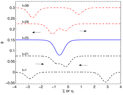
Figure 1: (Color online) Time evolution of two counter-propagating solitons for $\sigma=0.2$, $\epsilon=0.1$, $\delta=1.031$ and $\mu=-20$. Different colour corresponds to three different stages (before collision, during collision and after collision) of propagation.

It should be mentioned here that since the PLK perturbation technique makes use of the decomposition, $\phi_{1}=\Phi_{1}\left(\xi,\tau\right)+\Phi_{2}\left(\eta,\tau\right)$ (see Eq. 19), of wave potential fluctuations amounting to a linear superposition of KdV solitons (Eq. 37 and Eq. 38), it may not provide an accurate description of the amplitude dynamics during the collision process when the two solitons overlap. However the resultant phase shift is quite accurately determined within the perturbation limits since it involves an aymptotic calculation with the solitons well separated from each other. This fact has been well demonstrated and the technique successfully employed by several past authors studying head on collision of two solitary waves in various media xue ; ghosh ; versh ; labany . For a detailed critique of the strengths and limitations of the method the reader is referred to the paper by Verheest et al. versh .
Our main objective in this work is to assess the influence of strong coupling on these phase shifts and in the next section we present our results obtained using the above analytic relations (Eq. 43 and Eq. 44) for various plasma parameters.

III Results and Discussions

$\Phi_{1}(\xi,\tau)$ and $\Phi_{2}(\eta,\tau)$ are evaluated by solving the above KdV equations (Eq. (33) and (34)). The time evolution of these two solitary waves which propagate towards each other can be plotted by replacing $\Phi_{1}$ and $\Phi_{2}$ in Eq. (19). Fig. 1 shows the time evolution of two counter propagating solitons travelling with different amplitudes and widths. It is noticed that the DA solitary wave with higher amplitude travels faster than that of smaller amplitude which was also observed experimentally Pintu . It is worth mentioning that we have used $\epsilon=0.1$ in our calculations similar to Xue et al.xue .

The waves which are coming towards each other, penetrate and slightly dip immediately after the collision and return to their initial amplitudes at a later time.

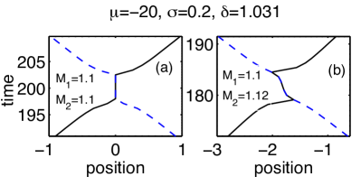
Figure 2: (Color online) Trajectory of solitons of (a) same ($M_{1}=M_{2}=1.1$) and (b) different ($M_{1}=1.1$ and $M_{2}=1.12$) amplitudes/Mach numbers. The solid and dashed lines represent the trajectory of soliton A and soliton B, respectively. The dusty plasma parameter are taken as $\mu=-20$, $\sigma=0.2$ and $\delta=1.031$.

Fig. 2 shows the trajectories of two counter propagating solitons with identical (see Fig. 2(a)) and with different Mach numbers (see Fig. 2(b)) respectively. It is to be noted that different Mach numbers imply different amplitudes with higher Mach numbers corresponding to larger amplitudes. As can be seen the phase diagram changes significantly when the amplitudes differ from each other. It is clear from Fig. 2(b) that the soliton with larger amplitude (soliton B) forces the other soliton with smaller amplitude (soliton A) to take a longer time to recover its shape after the collision. Hence it can be concluded that the phase shift of the smaller soliton is comparatively larger than that of the bigger one.

Since soliton A is travelling to the right and soliton B is travelling to the left, it is seen from Eqs. (43) and (44) that each soliton has a positive (or negative) phase shift in its traveling direction due to the collision. The sign of phase shift depends on the dusty plasma parameters mainly on $\delta$ and $\mu$ which will be discussed in more details later in this section.

It is clearly seen from Eqs. (43) and (44) that the phase shifts depend on the dusty plasma parameters (i.e. $\delta,\mu$ and $\sigma$) and the initial amplitudes of the two solitary waves ($\Phi_{A}~{}\text{and}~{}\Phi_{B})$. The co-efficient ‘$a$’ remains negative whereas the coefficients ‘$b$’ and ‘$d$’ remain positive for all the values of above mentioned parameters. But the co-efficient ‘$c$’ changes its sign for a particular set of these parameters. Since, the phase shift is directly proportional to ‘c’, its sign changes with the sign of ‘c’. A negative phase shift implies that the velocity of each soliton reduces at the time of the head-on collision li . It further signifies that they either travel the same distance in a longer time or a shorter distance in the same interval of time.

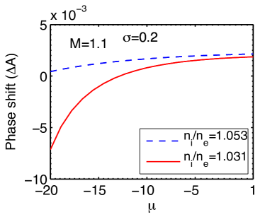
Figure 3: (Color online) Variation of phase shift of first soliton ($\Delta A$) with $\mu$ for different values of $\delta$ (dashed line and solid line represent $\delta=1.053$ and $\delta=1.031$, respectively.) at $\sigma=0.2$, $\epsilon=0.1$, $M=1.1$.

The variation of phase shift with compressibility ($\mu$) is shown in Fig. 3 for $\sigma=0.2$xue and $M=1.1$.

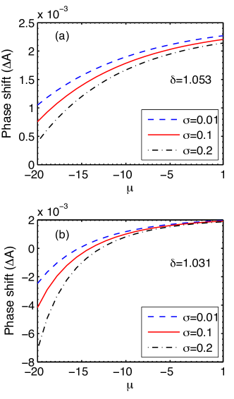
Figure 4: (Color online) Variation of phase shift $\Delta A$ with $\mu$ for (a) $\delta=1.053$ and (b) $\delta=1.031$. Dashed, solid and dash-doted lines represent $\sigma=0.01,\sigma=0.1$, and $\sigma=0.2$, respectively.

Our estimates for the phase shifts have been carried out for plasma parameters that are closely related to those of experiments done in the past for solitary waves. For example, in the experiment on soliton propagation carried out in Pintu the typical values of $\sigma$ and $\delta$ are $0.0375$ and $1.75$ respectively and they vary around these values with experimental changes of the discharge parameters. In another experimental paper by Sharma et al. bailung2014 , the typical values of these parameters are $\sigma=0.02$ and $\delta=1.1$. As stated in their paper, for different pressures, the value of the dust charge number changes and hence the value of $\delta$ changes. Our choice of parameter values are in the same range and therefore quite relevant for experimental investigations. Additionally, we have also varied the coupling parameter from the weakly coupled regime ($\Gamma<1$) to strongly coupled regime ($\Gamma>1$) to get the value of $\mu$ from the expression of the compressibility used in the manuscript (Eq. 5 and Eq. 6). Our choice of the range of the variation of the coupling parameter is also close to that reported in many experimental papers goree1 ; goree2 .

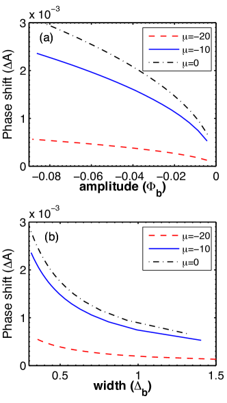
Figure 5: (Color online) Variation of phase shift $\Delta A$ with (a) amplitude($\Phi_{A}$) and (b) width($\Delta_{s}$) for three different values of $\mu$ ($\mu=-20$ (dashed), $\mu=-10$ (solid) and $\mu=0$ (dash-dotted)) at $\sigma=0.2$ and $\delta=1.053$.

To study the variations of phase shifts, we have plotted the phase shift of first solitary wave ($\Delta A$) against this parameters. It is not necessary to study the phase shift of the second soliton separately as it always shows the same trend as of the first one but with negative sign because it is travelling in the opposite direction. The solid and dashed lines depict for $\delta=n_{i}/n_{e}=1.031$ and $\delta=n_{i}/n_{e}=1.053$, respectively. It is clear from this figure that the phase shift changes significantly in strongly coupled regime ($\mu\leq 1$) compared to the weakly coupled regime ($\mu\geq 1$) for both the cases. Additionally, it is also seen that the phase shift ($\Delta A$) changes its sign for $\delta=1.031$ nearly at $\mu=-13$ for given dusty plasma parameters. It suggests that for both the cases, the velocity of soliton A reduces during collision because of higher rigidity of the medium that increases with the decrease of compressibility.

We have plotted the variation of phase shift with $\mu$ for $\sigma=$ 0.01 (dashed line), 0.1 (solid line) and 0.2 (dash-dotted line) in Fig. 4. We have chosen the value of $\delta=1.053$ in Fig. 4(a) whereas $\delta=1.031$ is chosen for Fig. 4(b). In case of Fig. 4(a), the phase shift is monotonically decreasing for each $\sigma$ with the increase of coupling parameter (decreasing $\mu$). But in Fig. 4(b), the magnitude of phase shift is initially decreasing (upto $\mu=-13$, as discussed in Fig. 3) and then it increases again with $\mu$. But for both the figures the velocity of soliton A is decreasing with the increase of the rigidity of the medium during collision. It is also found in both the cases that the phase delay decreases with the increase of temperature ratio, $\sigma$ for a given value of $\delta$.

Fig. 5 shows that the phase shift of soliton A changes significantly with the change of solitary amplitude of B and its width for three different values of $\mu$. It means for a given value of $\mu$, larger amplitude (or smaller width) of soliton B causes larger delay in the propagation of soliton A. This theoretical findings also supports the experimental results of Harvey et al. Harvey . For a given value of width (or amplitude) the phase-shift decreases with decrease of $\mu$. Decreasing $\mu$ corresponds to the increase of the rigidity of the medium.

IV Conclusion

We have theoretically calculated the leading-order phase shift resulting from a head-on collision between two counter propagating dust acoustic solitary waves in an unmagnetized strongly coupled dusty plasma system. The primary objective was to assess the influence of strong coupling on this nonlinear process. We have used the Generalized Hydrodynamic Equations to model the dust dynamics and accounted for strong coupling induced dispersive effects through modifications in the compressibility arising from contributions due to $\Gamma$. The variation of the phase shift as a function of the compressibility is studied. In addition the variation due to parameters like the density ratio ($\delta$), the temperature ratio ($\sigma$) of the plasma species and the initial amplitudes of the solitary waves on the phase delay are also investigated. We find that the phase shift from a head-on collision changes significantly in the strongly coupled regime as compared to the weakly coupled regime. We have also found that as we increase the rigidity of the medium the phase shift changes its sign for a given set of dusty plasma parameters. A negative phase shift suggests that the velocity of the solitary waves decreases at the time of the collision. It is also seen that the phase shift decreases with the increase of temperature ratio of ions to electrons. Further a larger amplitude (or smaller width) soliton causes a larger delay. Our model results may serve as interesting signatures of nonlinear manifestations of strong coupling effects that could be looked for in collision experiments in a laboratory set-up. They can also form the basis for further theoretical investigations where the effect of higher order corrections and dissipative contributions can be explored.

References

- (1) H. Ikezi, Phys. Fluids 29, 1764 (1986).
- (2) H. Thomas, G. E. Morfill, and V. Demmel, Phys. Rev. Lett. 73, 652-?655 (1994).
- (3) P. K. Shukla and V. P. Silin, Phys. Scr. 45, 508 (1992).
- (4) N. N. Rao, P. K. Shukla, and M. Y. Yu, Planet. Space Sci. 38, 543 (1990).
- (5) F. MelandsØ, Phys.Plasmas 3, 3890 (1996).
- (6) N. N. Rao, Phys.Plasmas 6, 4414 (1999).
- (7) D. Samsonov and J. Goree, Phys.Rev.E 59, 1047 (1999).
- (8) D. A. Law, W. H. Steel, B. M. Annaratone, and J. E. Allen, Phys. Rev. Lett. 80, 4189 (1998).
- (9) N. Rao and P. Shukla, Planet. Space Sci. 42, 221 (1994).
- (10) I. Kourakis and P. K. Shukla, Eur. Phys. J. D 29, 247 (2004).
- (11) G. E. Morfill and A. V. Ivlev, Rev. Mod. Phys. 81, 1353 (2009).
- (12) F. Verheest, Space Sci. Rev. 77, 267 (1996).
- (13) A. A. Mamun and P. K. Shukla, Phys. Scr., T98, 107 (2002).
- (14) D. Samsonov et al., Phys. Rev. Lett. 88, 095004 (2002).
- (15) P. Bandyopadhyay, G Prasad, A. Sen, and P.K. Kaw, Phys. Rev. Lett. 101, 065006 (2008).
- (16) R. Heidemann, S. Zhdanov, R. Sutterlin, H. M. Thomas, and G. E. Morfill, Phys. Rev. Lett 102, 135002 (2009).
- (17) N. J. Zabusky and M. D. Kruskal, Phys. Rev. Lett. 15, 240 (1965).
- (18) Hidekazu Tsuji and Masayuki Oikawa Fluid Dyn. Res. 42, 065506 (2010).
- (19) C. S. Gardner, J. M. Greener, M. D. Krushal, and M. Miura, Phys.Rev. Lett. 19, 1095 (1967).
- (20) J. K. Xue, Phys. Rev. E 69, 016403 (2004)
- (21) J. N. Han, X. X. Yang, D. Xiang Tian, and W. S Duan, Phys. Lett. A 372, 4817 (2008).
- (22) E. F. El-Shamy, Phys. Plasmas 16, 113704 (2009).
- (23) S. K. El- Labany, E. F. El-Shamy, W. F. El-Taibany, and P. K. Shukla, Phys. Lett. A 374, 960 (2010).
- (24) E. F. El-Shamy, W. M. Moslem, and P. K. Shukla, Phys. Lett. A 374, 290 (2009).
- (25) Frank Verheest, Manfblue A. Hellberg, Willy A. Hereman, Phys. Rev. E 86, 036402 (2012).
- (26) Uday Narayan Ghosh, Kaushik Roy, and Prasanta Chatterjee, Phys. Plasmas 18, 103703 (2011).
- (27) P. Harvey, C. Durniak, D., and G. Morfill Phys. Rev. E 81, 057401 (2010).
- (28) S. K. Sharma, A. Boruah, and H. Bailung, Phys. Rev. E 89, 013110 (2014).
- (29) P. K. Kaw and A.Sen, Phys. Plasmas 5, 3552 (1998).
- (30) A. Mishra, P. K. Kaw, and A. Sen, Phys. Plasmas 7, 3188 (2000).
- (31) B. M. Veeresha, S. K. Tiwari, A. Sen, P. K. Kaw, and A. Das Phys. Rev. E 81, 036407 (2010).
- (32) P. K. Shukla, A. A. Mamun, Introduction of Dusty Plasma Physics, IOP Publishing, London (2002).
- (33) P. Bandyopadhyay, G. Prasad, A. Sen, and P.K. Kaw Physics Letters A 368, 491 (2007).
- (34) J. Pramanik, G. Prasad, A. Sen, and P. K. Kaw Phys. Rev. Lett. 88, 175001 (2002).
- (35) P. Bandyopadhyay, G. Prasad, A. Sen, and P.K. Kaw Physics Letters A 372, 5467 (2008).
- (36) W. L. Slattery, G. D. Doolen, and H. E. DeWitt, Phys. Rev. A 21, 2087 (1980).
- (37) A. Jeffery and T. Kawahawa, Asymptotic Methods in Nonlinear Wave Theory (Pitman, London, 1982).
- (38) Guoxing Huang and Manuel G. Velarde, Phys. Rev. E 53, 2988 (1996).
- (39) T. Taniuti and C. C. Wei, J. Phys. Soc. Jpn. 24, 941 (1968).
- (40) T. Kakutani, H. Ono, T. Taniuti, and C.C. Wei, J. Phys. Soc. Jpn. 24, 1159 (1968).
- (41) S.C Li, Phys. Plasmas 17, 082307 (2010).
- (42) Z. Donkó, P. Hartmann and J. Goree, Modern Physics Letters B 21, 1357–1376 (2007)
- (43) V. Nosenko, J. Goree and A. Piel, Phys. Rev. Lett. 97, 115001 (2006)