A climate network-based index to discriminate different types of El Niño and La Niña
Abstract
El Niño exhibits distinct Eastern Pacific (EP) and Central Pacific (CP) types which are commonly, but not always consistently, distinguished from each other by different signatures in equatorial climate variability. Here, we propose an index based on evolving climate networks to objectively discriminate between both flavors by utilizing a scalar-valued evolving climate network measure that quantifies spatial localization and dispersion in El Niño’s associated teleconnections. Our index displays a sharp peak (high localization) during EP events, whereas during CP events (larger dispersion) it remains close to the baseline observed during normal periods. In contrast to previous classification schemes, our approach specifically account for El Niño’s global impacts. We confirm recent El Niño classifications for the years 1951 to 2014 and assign types to those cases were former works yielded ambiguous results. Ultimately, we study La Niña episodes and demonstrate that our index provides a similar discrimination into two types.
Geophysical Research Letters
Potsdam Institute for Climate Impact Research — Telegrafenberg A 31, 14412 Potsdam, Germany, EU Department of Physics, Humboldt University — Newtonstraße 15, 12489 Berlin, Germany, EU Mercator Research Institute on Global Commons and Climate Change — Torgauer Straße 12-15, 10829 Berlin, Germany, EU Economics of Climate Change, Technical University — Straße des 17. Juni 145, 10623 Berlin, Germany, EU Stockholm Resilience Centre, Stockholm University — Kräftriket 2B, 114 19 Stockholm, Sweden, EU Institute for Complex Systems and Mathematical Biology, University of Aberdeen — Aberdeen AB24 3FX, UK, EU Department of Control Theory, Nizhny Novgorod State University — Gagarin Avenue 23, 606950 Nizhny Novgorod, Russia
Marc Wiedermannmarcwie@pik-potdam.de
Discrimination between Eastern and Central Pacific El Niño
New index based on climate networks for objective classification
Discriminations are possible for La Niña as well
1 Introduction
The El Niño Southern Oscillation (ENSO) alternates between positive (El Niño) and negative (La Niña) phases (Trenberth, 1997). Especially the El Niño phase further exhibits two distinct types characterized by different spatial patterns of SST anomalies (e.g., Ashok et al., 2007; Kao and Yu, 2009; Kug et al., 2009; Yeh et al., 2009). The first type (the classic or Eastern Pacific (EP) El Niño (Rasmusson and Carpenter, 1982; Harrison and Larkin, 1998)) is characterized by strong positive SST anomalies close to the western coast of South America, while the second type (referred to as El Niño Modoki or Central Pacific (CP) El Niño by different authors) exhibits the strongest SST anomalies close to the dateline. Both types cause different impacts on the global climate system, such as increased rainfall over north and eastern Australia during CP El Niños (Ashok et al., 2007; Taschetto and England, 2009) contrasted by a rainfall reduction over eastern Australia during EP El Niños (Chiew et al., 1998). Thus, a proper discrimination of these types provides key information to assess El Niño’s possible impacts on other climate subsystems.
While recent literature shows a large agreement on the classification of many El Niños, contradictory classifications arise in certain years such as, e.g., 1986/1987, which has been classified as mixed (Kug et al., 2009), EP (Kim et al., 2011; Yeh et al., 2009; Hu et al., 2011) or CP (Larkin and Harrison, 2005; Hendon et al., 2009; Graf and Zanchettin, 2012). In fact, when reviewing existing studies (Kim et al., 2009; Kug et al., 2009; Kim et al., 2011; Yeh et al., 2009; Hu et al., 2011; Larkin and Harrison, 2005; Hendon et al., 2009; Graf and Zanchettin, 2012), 8 out of 19 El Niño events between 1957 and 2010 have not been classified in agreement. These mismatches possibly arise since most discrimination schemes indeed utilize the same climate observable (mostly SST), but apply different derived characteristics such as the ENSO Modoki Index (EMI) (Ashok et al., 2007), the Nino3 and Nino4 index (Kim et al., 2011; Hu et al., 2011), or empirical orthogonal function (EOF) analysis (Kao and Yu, 2009; Graf and Zanchettin, 2012) to distinguish both El Niño types.
To provide a consistent and systematic discrimination, we propose here a method to distinguish the two different El Niño types based on the assessment of time evolving complex climate networks (Radebach et al., 2013). Climate networks consist of nodes representing time series and links displaying some statistically relevant interdependency between them (Donges et al., 2009a; Tsonis et al., 2006) ENSO has been studied intensively using this tool to quantify corresponding teleconnections (Gozolchiani et al., 2011; Tsonis and Swanson, 2008; Tsonis et al., 2008) and its effect on other climatic subsystems (Gozolchiani et al., 2008). Recently, climate network approaches allowed for successfully forecasting El Niño by assessing the strength of linkages in the equatorial Pacific (Ludescher et al., 2013, 2014).
Radebach et al. (2013) systematically studied the temporal evolution of a global climate network in a spatially explicit way and linked the resulting variability of its topology to the presence of the two different El Niño types. Following these lines of thought we develop a thorough classification scheme that allows for an objective discrimination between EP and CP El Niños. While most previous studies on El Niño classification focus on climate variability only within the equatorial Pacific, we specifically acknowledge the global impact of ENSO. Our framework therefore accounts for the correlation structure of global surface air temperature anomalies (SATA), a variable that is highly affected by El Niño (Yamasaki et al., 2008) and is, in contrast to SST, available homogeneously sampled for the entire globe.
As an index that discriminates EP and CP El Niños, we utilize the climate network’s transitivity, a scalar-valued measure, that quantifies the (disperse vs. strongly localized) spatial distribution of pairwise correlations and teleconnections along the globe. First, we assess whether a certain period displays El Niño conditions according to the Oceanic Niño Index (ONI). Second, we determine the transitivity of evolving climate networks computed from one-year running window cross-correlations with respect to a baseline value defined by the transitivity of networks computed from 30-year windows that are centered around the period of interest. The surpassing of that threshold defines an EP El Niño, while the contrary case indicates a CP El Niño. In comparison with recent studies, our methods confirms all EP and CP El Niños between 1951 and 2014 that were commonly defined by Kug et al. (2009); Kim et al. (2011); Yeh et al. (2009); Hu et al. (2011); Larkin and Harrison (2005); Hendon et al. (2009) and Graf and Zanchettin (2012) and provides a consistent classification for those periods that were ambiguously classified so far.
To consolidate our findings, we provide results for the climate network’s node strength fields during periods that our index defines as EP or CP El Niños and show their similarity with patterns that are expected from an EOF analysis (Johnson, 2013; Donges et al., 2015a). As recent works (Kug and Ham, 2011; Yuan and Yan, 2012; Tedeschi et al., 2013) addressed the issue whether two types of La Niña can be detected as well, we perform the same procedure for these events and provide a similar discrimination for the negative phase of ENSO.
2 Data
We define El Niño periods according to the Oceanic Niño Index (ONI) provided by the Climate Prediction Center of the National Oceanic and Atmospheric Administration, which covers the time between 1950 and 2015 and is computed as the 3-month running mean SST anomaly in the Nino3.4 region (N-S, W-W) with respect to centered 30-year base periods that are updated every 5 years. As the initial and final year of this data set include only incomplete information on the 1951 La Niña and the 2015 El Niño, we restrict ourselves to the period from 1951 to 2014.
We construct evolving climate networks from daily global surface air temperature (SAT) data provided by the NCEP/NCAR reanalysis (Kistler et al., 2001) with a spatial resolution of in longitudinal and latitudinal direction covering the same time period as the ONI. All 288 grid points located at the poles and all leap days are removed. The data is anomalized in accordance with the definition of the ONI by subtracting from the time series at every grid point the long-term annual cycle computed over the same 30-year base periods as above that are updated every 5 years. Due to the lack of data before 1948 and after 2015, the years 1951 to 1965 are anomalized by the same base period (1951–1980) as the years 1965 to 1969. Similarly, the years 2005 to 2015 are anomalized by the 1986 to 2015 base period. We acknowledge that this procedure induces small offsets in the time series after every 5 years. However, as we construct evolving climate networks from time series of much shorter length we neglect these effects for the sake of consistency with the definition of the ONI. The above anomalization process ensures that once defined anomalies and ENSO periods are not altered by the addition of more recent data.
Finally, we obtain time series of surface air temperature anomalies (SATA) with temporal sampling points each.
3 Methods
A climate network consists of a set of nodes that correspond to the grid points in the underlying data set and a set of links which connect pairs of nodes and indicate a strong statistical interrelationship between them. The network is represented by its binary adjacency matrix A with entries if two nodes and are linked and otherwise (Donges et al., 2009b; Boers et al., 2013; Stolbova et al., 2014). An extension of this procedure is the usage of an edge-weighted adjacency matrix W where denotes the absence of a link, but denotes its strength (e.g., the pairwise correlation) (Barrat et al., 2004; Hlinka et al., 2014; Zemp et al., 2014).
3.1 Network construction
Following the framework of evolving climate network analysis (Radebach et al., 2013; Hlinka et al., 2014) we construct a sequence of networks from running-window cross-correlation matrices between all pairs of SATA time series. A window is characterized by its size and offset to the previous window. We choose days and days to ensure that each window covers at least the entire duration of an El Niño or La Niña episode. For each window we obtain the truncated time series and compute the resulting cross-correlation matrix . In accordance with previous studies (Donges et al., 2009a; Tsonis et al., 2006; Paluš et al., 2011), we rely here on the linear Pearson correlation at zero lag.
To reduce the complexity of , it is advisable to represent only a certain fraction of strongest absolute correlations as links between the nodes (Tsonis et al., 2006; Donges et al., 2009a). This yields an individual threshold for each absolute correlation matrix above which nodes are treated as linked. is then called the link density of . Here, we keep fixed for all windows . This choice gives a number of links as low as possible to ensure the consideration of only the strongest correlations. Further, roughly corresponds to the fraction of nodes that are situated inside the the Nino3.4 region. We obtain thresholds (i.e., the lower bound of absolute correlations values) in the range of 0.53 to 0.65. They are significant above the significance level according to a standard student’s t-test.
Binarizing to an edge-unweighted adjacency matrix would neglect valuable information on the varying strength of correlation between connected grid points. We therefore compute edge-weighted adjacency matrices with entries if two nodes are are linked,
| (1) |
Due to the underlying grid type, the density of nodes increases towards the poles inducing a systematic bias into the computation of network measures (Heitzig et al., 2012). This effect is corrected by assigning each node a weight corresponding to its latitudinal position on the grid (Tsonis et al., 2006; Heitzig et al., 2012; Wiedermann et al., 2013),
| (2) |
Network measures that include have been referred to as node splitting invariant (n.s.i.) measures (Heitzig et al., 2012; Zemp et al., 2014; Wiedermann et al., 2013).
3.2 Network transitivity
El Niño has a global impact on the climate system manifested by long-ranging teleconnections into different regions of the Earth (Held et al., 1989; Neelin, 2003; Trenberth, 1997) which, in the context of climate networks can be regarded as mediators of variations and fluctuations (Tsonis et al., 2008; Runge et al., 2015). Thus, El Niño and its teleconnections cause a spatial organization of high co-variability along the Earth’s surface, which is reflected in the resulting climate network. The degree of this organization can be quantified by a single-valued scalar metric, the network transitivity (Watts and Strogatz, 1998; Saramäki et al., 2007), which we use in its node-weighted form (Heitzig et al., 2012),
| (3) |
gives the edge- and node-weighted fraction of closed triangles between triples of nodes and measures how strongly the correlation in a system under study or subsets thereof is spatially organized (high values) or dispersed (low values). In a purely random network, would naturally take very low values, i.e., approximately equal the link density in the standard case of no specific edge and node-weights (Erdős and Rényi, 1960). thus serves as a good discriminator between phases of strong localization and high dispersion in the global teleconnectivity of evolving climate networks (Radebach et al., 2013). As EP and CP El Niños have been shown to display different characteristics in their associated teleconnections (Ashok et al., 2007) we expect to respond differently to the presence of either of the two types.
3.3 Strength of individual nodes
To connect our work with previous results from statistical climatology we investigate for each node its corresponding area-weighted strength
| (4) |
individually for each network . measures the total weight of links that are attached to each node . For the edge-unweighted case, this measure reduces to the area-weighted connectivity (Tsonis et al., 2008) which displays striking similarity with results from a node-weighted EOF analysis (Donges et al., 2015a; Wiedermann et al., 2015).
4 Results
The ONI identifies El Niño (La Niña) episodes if its values exceed (fall below) a threshold of 0.5K (-0.5K) for at least 5 consecutive months, yielding 22 (18) El Niño (La Niña) episodes between 1951 and 2014 (Fig. 1A).
4.1 Transitivity
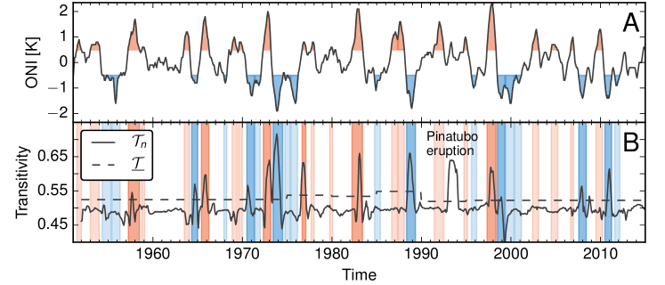
We construct evolving climate networks and compute their transitivity and node strength . The end point of each window marks the time at which the two measures are evaluated. Figure 1B shows the evolution of . Except for one case with several 12-month time windows ending in 1993, which is likely caused by the eruption of Mount Pinatubo in 1991 (McCormick et al., 1995; Radebach et al., 2013), distinct peaks in coincide exclusively with certain ENSO episodes. As shown by Radebach et al. (2013), the presence of an EP El Niño likely coincides with strong signals in (for their case unweighted) transitivity, while no distinct signal is present during CP El Niños. However, no quantitative criterion for this discrimination has been given so far.
To give an objective definition of a strong transitivity signal we define a threshold value above which is considered to display a peak. We obtain an adaptive value of as the transitivities of climate networks constructed for the same 30-year periods that were used for the anomalization of the SAT data and the derivation of the ONI. Thus, we compare all values of computed, e.g., during the period 1975–1979 with a baseline transitivity computed for a climate network covering the 30-year period of 1961–1990 (dashed line in Fig 1B). This procedure follows the definition of the ONI and we interpret as representing the long-term average spatial organization in the global climate network. Adaptively updating every 5 years automatically accounts for possible effects of long-term climate change trends imprinting on the network statistics and the definition of for periods in the past is not affected by the addition of more recent data.
We detect six El Niño periods during which crosses (dark red areas in Fig. 1B) corresponding to the El Niños of 1957, 1965, 1972, 1976, 1982, and 1997. For all other El Niños stays below . In the scope of our framework, we thus propose classifying the first case as EP and the second case as CP events (light red areas in Fig. 1B).
| Kug et al. | Kim et al. | Hu et al. | Larkin et al. | Hendon et al. | Graf et al. | Yeh et al. | Kim et al. | Common | Full | |
|---|---|---|---|---|---|---|---|---|---|---|
| (2009) | (2011) | (2011) | (2005) | (2009) | (2012) | (2009) | (2009) | results | ||
| 1953/1954 | - | - | - | - | - | - | - | - | - | CP |
| 1957/1958 | - | - | EP | EP | - | EP | EP | EP | EP | EP |
| 1958/1959 | - | - | - | - | - | - | - | - | - | CP |
| 1963/1964 | - | - | - | CP | - | CP | EP | EP | - | CP |
| 1965/1966 | - | - | EP | EP | - | EP | EP | EP | EP | EP |
| 1968/1969 | - | - | CP | CP | - | CP | CP | - | CP | CP |
| 1969/1970 | - | - | EP | EP | - | - | EP | CP | - | CP |
| 1972/1973 | EP | EP | EP | EP | - | EP | EP | EP | EP | EP |
| 1976/1977 | EP | EP | - | EP | - | EP | EP | EP | EP | EP |
| 1977/1978 | CP | CP | - | CP | - | CP | CP | - | CP | CP |
| 1979/1980 | - | - | - | - | - | - | * | - | - | CP |
| 1982/1983 | EP | EP | EP | EP | EP | EP | EP | EP | EP | EP |
| 1986/1987 | * | EP | EP | CP | CP | CP | EP | - | - | CP |
| 1987/1988 | * | - | CP | EP | EP | - | EP | EP | - | CP |
| 1991/1992 | * | EP | EP | EP | CP | CP | EP | CP | - | CP |
| 1994/1995 | CP | CP | CP | CP | CP | CP | CP | CP | CP | CP |
| 1997/1998 | EP | EP | EP | EP | EP | EP | EP | EP | EP | EP |
| 2002/2003 | CP | CP | CP | EP | CP | CP | * | CP | - | CP |
| 2004/2005 | CP | CP | - | - | CP | CP | CP | CP | CP | CP |
| 2006/2007 | - | EP | CP | CP | - | - | EP | - | - | CP |
| 2009/2010 | - | CP | - | - | - | CP | - | - | CP | CP |
| TPR | 1.0 | 0.57 | 0.62 | 0.6 | 0.67 | 1.0 | 0.5 | 0.75 | 1.0 |
For comparison, the proposed classifications of El Niño phases into EP and CP types from eight recent studies (Kim et al., 2009; Kug et al., 2009; Kim et al., 2011; Yeh et al., 2009; Hu et al., 2011; Larkin and Harrison, 2005; Hendon et al., 2009; Graf and Zanchettin, 2012) are summarized in Tab. 1. To quantify the consistency of the network-based discrimination, we define a true positive rate (TPR) as the fraction of EP El Niños in each study that are detected by our framework. Accordingly, the false positive rate (FPR) is the fraction of CP El Niños in each study that our method classifies as EP type. With respect to all references we obtain a FPR of zero. The TPR for each reference is presented in the last row of Tab. 1. Its values vary between 1 for the comparison with Graf and Zanchettin (2012) and Hu et al. (2011), and 0.5 for the comparison with Yeh et al. (2009). Furthermore, we note that among all references 8 out of 19 events are not classified in agreement. Taking only the mutual agreement between all references as a basis for testing, we confirm all past classifications (second-last column in Tab. 1). To provide results for the eight ambiguously defined periods, the network-based classification for all El Niños is given in the last column of Tab. 1.
We find the largest consistency with the results from Graf and Zanchettin (2012) which are obtained from an EOF analysis, a framework that, like our method, is based on the evaluation of cross-correlations between different grid points. This methodological congruence may explain the good agreement between the results and confirms the validity of our work. However, the advantage of utilizing a network-based approach instead of EOFs is that the entire spatial structure of the underlying covariance patterns is reduced to a single index. Moreover, its evaluation does not rely on any visual inspection, but provides an objective binary classification depending on whether or not the short-term transitivity exceeds its long-term baseline .
We repeat the analysis for La Niña periods and classify 7 EP (1964, 1970, 1973, 1988, 1998, 2007, 2010) and 11 CP (1954, 1955, 1967, 1971, 1974, 1975, 1984, 1995, 2000, 2001, and 2011) periods (dark (EP) and light (CP) blue areas in Fig. 1B). Even though references providing actual discriminations of the different La Niña years are scarse, we compiled two recent works and confirm the reported EP La Niñas of 1964 and 1970 (Yuan and Yan, 2012) and CP La Niñas of 1975, 1984, 2000, 2001, and 2011 (Yuan and Yan, 2012; Tedeschi et al., 2013). Future work should further evaluate the discrimination of La Niña periods proposed by our method.
4.2 Node strength
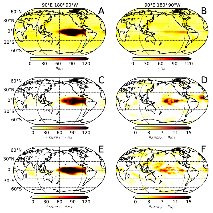
To further consolidate our findings we compute the average node strengths from the six networks that are used to define (Fig. 2A). We obtain the highest values in the equatorial Pacific highlighting ENSO’s importance in the global climate network. Additionally, we compute the average node strength taken over all normal periods, i.e., those periods where neither El Niño or La Niña are present (Fig. 2A). As by its definition the effect of ENSO is reduced, displays comparably low values and a more homogeneous distribution across the entire globe than . Ultimately, we calculate the average node strength () taken over all El Niño periods that our method classifies as EP (CP) type (see also Fig. 1B). To investigate the deviation from the normal state during either of the two periods we display their differences from in Fig. 2C,D. For EP El Niños (Fig. 2C) we find an expected maximum in the equatorial Pacific, which is the typical ENSO-related pattern known from a classical EOF analysis (Johnson, 2013). For CP El Niños we find a weakening of this pattern and a westward shift of the maxima towards the dateline. This pattern has been observed in the corresponding EOFs as well (Johnson, 2013). However, we note that only differs from to a small amount (Fig. 2D). This again suggests, that during CP El Niños the evolving climate networks exhibit a similar state as during normal periods. We compute similar average quantities, and , for La Niña events and again evaluate their deviations from the normal state (Fig. 2E,F). We find quantitatively and qualitatively similar patterns as for El Niño, which highlights the symmetry in the statistics of the two ENSO phases. Even though a similarly thorough comparison with existing literature is not yet possible for La Niña, the high congruence between and ( and ) suggests that our discrimination scheme provides reasonable results for La Niña phases as well.
4.3 Robustness
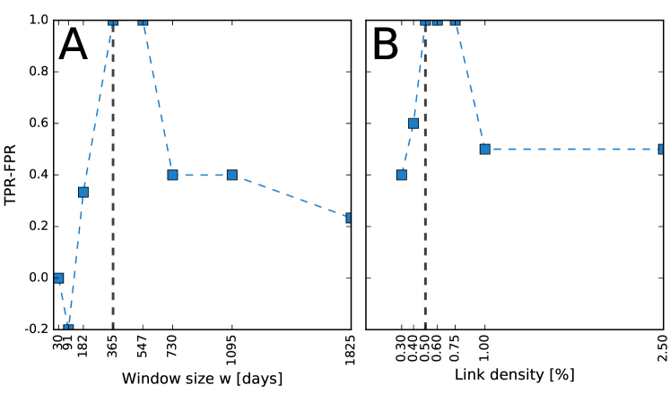
To evaluate the robustness of our results with respect to the window size and link density , we vary both parameters individually and assess the difference between the TPR and FPR when testing our classification against the largest overlap of the literature (second-last column in Tab. 1). This score takes its maximum value of if our method confirms the literature’s classification of each event and is lower otherwise. Figure 3A (Fig. 3B) shows the score for different () and fixed ( days). The highest scores are obtained for window sizes between and days and link densities between and . Shorter window sizes cause a reduction of the score as the windows become too small to sufficiently cover the temporal extent of an ENSO event. For larger window sizes the effect of ENSO is suppressed by including too many of the normal periods into each window. The link density of was initially chosen as it roughly corresponds to the fraction of nodes located inside the Nino3.4 region. Smaller values cause the network to be only composed of highly correlated trivial nearest-neighbor connections and teleconnections with comparably lower pairwise cross-correlation vales are not captured. In contrast, larger values result in too many trivial links alongside those attributed to the effects of ENSO. Generally, the score varies smoothly along the range of parameters and shows maximum values for our initial choices. Thus, we consider our results to be sufficiently robust.
5 Conclusion
We have proposed an index based on evolving climate networks to objectively discriminate between EP and CP types of El Niño and La Niña episodes. It relies on the evolution of the networks’ transitivity, measuring spatial localization and dispersion of strong cross-correlations between different grid points in a global SATA field. If this index peaks during an ENSO phase, it detects the presence of an EP type event. In contrast, the absence of a remarkable signal during an ENSO period indicates CP type events. From the climate network perspective this indicates an increased localization and clustering of teleconnections during EP phases in comparison with CP and normal phases where teleconnections seem to appear more dispersed. Our method does not require any visual inspection or manual thresholding of observed patterns but objectively categorizes ENSO phases into different types by intercomparing the networks’ short-term () and long-term states ().
In comparison with eight recent works on El Niño classification our method confirms the classification of years that all references have in common and provides a discrimination for those years that where so far ambiguously defined. Compared to approaches based on average temperature observations our method produces a sharp signal in the variable under study, i.e, the network transitivity, and thus provides a clear distinction between the two types of El Niño episodes.
Even though references are scarce, our findings also confirm different recently reported EP and CP La Niña periods and show that our discrimination scheme is applicable to this negative phase of ENSO as well.
Future work should investigate more thoroughly the spatial distribution of links in the evolving climate networks during different ENSO stages to gain a more systematic understanding of the physical mechanisms behind the observed differences in transitivity. Moreover, being automated and objective, our framework allows for a systematic evaluation of climate model simulations and could be used to investigate potential changes in the projected frequency of the two ENSO flavors in the future, e.g., due to anthropogenic global warming (Yeh et al., 2009).
Acknowledgements.
MW and RVD have been supported by the German Federal Ministry for Education and Research via the BMBF Young Investigators Group CoSy-CC2 (grant no. 01LN1306A). JFD thanks the Stordalen Foundation via the Planetary Boundary Research Network (PB.net) and the Earth League’s EarthDoc programme for financial support. JK acknowledges the IRTG 1740 funded by DFG and FAPESP. NCEP Reanalysis data is provided by the NOAA/OAR/ESRL PSD, Boulder, Colorado, USA, from their website http://www.esrl.noaa.gov/psd/. Parts of the analysis have been performed using the Python package pyunicorn (Donges et al., 2015b) available at https://github.com/pik-copan/pyunicorn.References
- Ashok et al. (2007) Ashok, K., S. K. Behera, S. A. Rao, H. Weng, and T. Yamagata (2007), El Niño Modoki and its possible teleconnection, J. Geophys. Res., 112(C11), C11007, 10.1029/2006JC003798.
- Barrat et al. (2004) Barrat, A., M. Barthélemy, R. Pastor-Satorras, and A. Vespignani (2004), The architecture of complex weighted networks, Proc. Natl. Acad. Sci. USA, 101(11), 3747–3752, 10.1073/pnas.0400087101.
- Boers et al. (2013) Boers, N., B. Bookhagen, N. Marwan, J. Kurths, and J. Marengo (2013), Complex networks identify spatial patterns of extreme rainfall events of the South American Monsoon System, Geophys. Res. Lett., 40(16), 4386–4392, 10.1002/grl.50681.
- Cai et al. (2015) Cai, W., A. Santoso, G. Wang, S.-W. Yeh, S.-I. An, K. M. Cobb, M. Collins, E. Guilyardi, F.-F. Jin, J.-S. Kug, M. Lengaigne, M. J. McPhaden, K. Takahashi, A. Timmermann, G. Vecchi, M. Watanabe, and L. Wu (2015), ENSO and greenhouse warming, Nature Clim. Change, 5(9), 849–859, 10.1038/nclimate2743.
- Chiew et al. (1998) Chiew, F. H. S., T. C. Piechota, J. A. Dracup, and T. A. McMahon (1998), El Niño/Southern Oscillation and Australian rainfall, streamflow and drought: Links and potential for forecasting, J. Hydrol., 204(1–4), 138–149, 10.1016/S0022-1694(97)00121-2.
- Donges et al. (2009a) Donges, J. F., Y. Zou, N. Marwan, and J. Kurths (2009a), Complex networks in climate dynamics, Eur. Phys. J. Spec. Top., 174(1), 157–179, 10.1140/epjst/e2009-01098-2.
- Donges et al. (2009b) Donges, J. F., Y. Zou, N. Marwan, and J. Kurths (2009b), The backbone of the climate network, Europhys. Lett., 87(4), 48,007, 10.1209/0295-5075/87/48007.
- Donges et al. (2015a) Donges, J. F., I. Petrova, A. Loew, N. Marwan, and J. Kurths (2015a), How complex climate networks complement eigen techniques for the statistical analysis of climatological data, Clim. Dyn., 9(45), 2407–2424, 10.1007/s00382-015-2479-3.
- Donges et al. (2015b) Donges, J. F., J. Heitzig, B. Beronov, M. Wiedermann, J. Runge, Q. Y. Feng, L. Tupikina, V. Stolbova, R. V. Donner, N. Marwan, H. A. Dijkstra, and J. Kurths (2015b), Unified functional network and nonlinear time series analysis for complex systems science: The pyunicorn package, Chaos, 25(11), 113,101, 10.1063/1.4934554.
- Erdős and Rényi (1960) Erdős, P., and A. Rényi (1960), On the evolution of random graphs, Publ. Math. Inst. Hung. Acad. Sci, 5, 17–61.
- Gozolchiani et al. (2008) Gozolchiani, A., K. Yamasaki, O. Gazit, and S. Havlin (2008), Pattern of climate network blinking links follows El Niño events, Europhys. Lett., 83(2), 28,005, 10.1209/0295-5075/83/28005.
- Gozolchiani et al. (2011) Gozolchiani, A., S. Havlin, and K. Yamasaki (2011), Emergence of El Niño as an Autonomous Component in the Climate Network, Phys. Rev. Lett., 107(14), 148501, 10.1103/PhysRevLett.107.148501.
- Graf and Zanchettin (2012) Graf, H.-F., and D. Zanchettin (2012), Central Pacific El Niño, the “subtropical bridge,” and Eurasian climate, J. Geophys. Res., 117(D1), D01102, 10.1029/2011JD016493.
- Harrison and Larkin (1998) Harrison, D. E., and N. K. Larkin (1998), El Niño-Southern Oscillation sea surface temperature and wind anomalies, 1946–1993, Rev. Geophys., 36(3), 353–399, 10.1029/98RG00715.
- Heitzig et al. (2012) Heitzig, J., J. F. Donges, Y. Zou, N. Marwan, and J. Kurths (2012), Node-weighted measures for complex networks with spatially embedded, sampled, or differently sized nodes, Eur. Phys. J. B, 85(1), 1–22, 10.1140/epjb/e2011-20678-7.
- Held et al. (1989) Held, I. M., S. W. Lyons, and S. Nigam (1989), Transients and the Extratropical Response to El Niño, J. Atmos. Sci., 46(1), 163–174, 10.1175/1520-0469(1989)046¡0163:TATERT¿2.0.CO;2.
- Hendon et al. (2009) Hendon, H. H., E. Lim, G. Wang, O. Alves, and D. Hudson (2009), Prospects for predicting two flavors of El Niño, Geophys. Res. Lett., 36(19), L19,713, 10.1029/2009GL040100.
- Hlinka et al. (2014) Hlinka, J., D. Hartman, N. Jajcay, M. Vejmelka, R. Donner, N. Marwan, J. Kurths, and M. Paluš (2014), Regional and inter-regional effects in evolving climate networks, Nonlinear Proc. Geophys., 21(2), 451–462, 10.5194/npg-21-451-2014.
- Hu et al. (2011) Hu, Z.-Z., A. Kumar, B. Jha, W. Wang, B. Huang, and B. Huang (2011), An analysis of warm pool and cold tongue El Niños: air–sea coupling processes, global influences, and recent trends, Clim. Dyn., 38(9-10), 2017–2035, 10.1007/s00382-011-1224-9.
- Johnson (2013) Johnson, N. C. (2013), How Many ENSO Flavors Can We Distinguish?, J. Climate, 26(13), 4816–4827, 10.1175/JCLI-D-12-00649.1.
- Kao and Yu (2009) Kao, H.-Y., and J.-Y. Yu (2009), Contrasting Eastern-Pacific and Central-Pacific Types of ENSO, J. Climate, 22(3), 615–632, 10.1175/2008JCLI2309.1.
- Kim et al. (2009) Kim, H.-M., P. J. Webster, and J. A. Curry (2009), Impact of Shifting Patterns of Pacific Ocean Warming on North Atlantic Tropical Cyclones, Science, 325(5936), 77–80, 10.1126/science.1174062.
- Kim et al. (2011) Kim, W., S.-W. Yeh, J.-H. Kim, J.-S. Kug, and M. Kwon (2011), The unique 2009–2010 El Niño event: A fast phase transition of warm pool El Niño to La Niña, Geophys. Res. Lett., 38(15), L15,809, 10.1029/2011GL048521.
- Kistler et al. (2001) Kistler, R., W. Collins, S. Saha, G. White, J. Woollen, E. Kalnay, M. Chelliah, W. Ebisuzaki, M. Kanamitsu, V. Kousky, H. van den Dool, R. Jenne, and M. Fiorino (2001), The NCEP–NCAR 50–Year Reanalysis: Monthly Means CD–ROM and Documentation, Bull. Amer. Meteor. Soc., 82(2), 247–267, 10.1175/1520-0477(2001)082¡0247:TNNYRM¿2.3.CO;2.
- Kug and Ham (2011) Kug, J.-S., and Y.-G. Ham (2011), Are there two types of La Nina?, Geophys. Res. Lett., 38(16), L16,704, 10.1029/2011GL048237.
- Kug et al. (2009) Kug, J.-S., F.-F. Jin, and S.-I. An (2009), Two Types of El Niño Events: Cold Tongue El Niño and Warm Pool El Niño, J. Climate, 22(6), 1499–1515, 10.1175/2008JCLI2624.1.
- Larkin and Harrison (2005) Larkin, N. K., and D. E. Harrison (2005), Global seasonal temperature and precipitation anomalies during El Niño autumn and winter, Geophys. Res. Lett., 32(16), L16,705, 10.1029/2005GL022860.
- Ludescher et al. (2013) Ludescher, J., A. Gozolchiani, M. I. Bogachev, A. Bunde, S. Havlin, and H. J. Schellnhuber (2013), Improved El Niño forecasting by cooperativity detection, Proc. Natl. Acad. Sci. USA, 110(29), 11,742–11,745, 10.1073/pnas.1309353110.
- Ludescher et al. (2014) Ludescher, J., A. Gozolchiani, M. I. Bogachev, A. Bunde, S. Havlin, and H. J. Schellnhuber (2014), Very early warning of next El Niño, Proc. Natl. Acad. Sci. USA, 111(6), 2064–2066, 10.1073/pnas.1323058111.
- McCormick et al. (1995) McCormick, M. P., L. W. Thomason, and C. R. Trepte (1995), Atmospheric effects of the Mt Pinatubo eruption, Nature, 373(6513), 399–404, 10.1038/373399a0.
- McPhaden et al. (2011) McPhaden, M. J., T. Lee, and D. McClurg (2011), El Niño and its relationship to changing background conditions in the tropical Pacific Ocean, Geophys. Res. Lett., 38(15), L15,709, 10.1029/2011GL048275.
- Neelin (2003) Neelin, J. D. (2003), Tropical drought regions in global warming and El Niño teleconnections, Geophys. Res. Lett., 30(24), 10.1029/2003GL018625.
- Paluš et al. (2011) Paluš, M., D. Hartman, J. Hlinka, and M. Vejmelka (2011), Discerning connectivity from dynamics in climate networks, Nonlinear Proc. Geophys., 18(5), 751–763, 10.5194/npg-18-751-2011.
- Radebach et al. (2013) Radebach, A., R. V. Donner, J. Runge, J. F. Donges, and J. Kurths (2013), Disentangling different types of El Niño episodes by evolving climate network analysis, Phys. Rev. E, 88(5), 052807, 10.1103/PhysRevE.88.052807.
- Rasmusson and Carpenter (1982) Rasmusson, E. M., and T. H. Carpenter (1982), Variations in Tropical Sea Surface Temperature and Surface Wind Fields Associated with the Southern Oscillation/El Niño, Mon. Wea. Rev., 110(5), 354–384, 10.1175/1520-0493(1982)110¡0354:VITSST¿2.0.CO;2.
- Runge et al. (2015) Runge, J., V. Petoukhov, J. F. Donges, J. Hlinka, N. Jajcay, M. Vejmelka, D. Hartman, N. Marwan, M. Paluš, and J. Kurths (2015), Identifying causal gateways and mediators in complex spatio-temporal systems, Nat. Commun., 6, 8502, 10.1038/ncomms9502.
- Saramäki et al. (2007) Saramäki, J., M. Kivelä, J.-P. Onnela, K. Kaski, and J. Kertész (2007), Generalizations of the clustering coefficient to weighted complex networks, Phys. Rev. E, 75(2), 027105, 10.1103/PhysRevE.75.027105.
- Stolbova et al. (2014) Stolbova, V., P. Martin, B. Bookhagen, N. Marwan, and J. Kurths (2014), Topology and seasonal evolution of the network of extreme precipitation over the Indian subcontinent and Sri Lanka, Nonlinear Proc. Geophys., 21(4), 901–917, 10.5194/npg-21-901-2014.
- Taschetto and England (2009) Taschetto, A. S., and M. H. England (2009), El Niño Modoki Impacts on Australian Rainfall, J. Climate, 22(11), 3167–3174, 10.1175/2008JCLI2589.1.
- Tedeschi et al. (2013) Tedeschi, R. G., I. F. A. Cavalcanti, and A. M. Grimm (2013), Influences of two types of ENSO on South American precipitation, Int. J. Climatol., 33(6), 1382–1400, 10.1002/joc.3519.
- Timmermann et al. (1999) Timmermann, A., J. Oberhuber, A. Bacher, M. Esch, M. Latif, and E. Roeckner (1999), Increased El Niño frequency in a climate model forced by future greenhouse warming, Nature, 398(6729), 694–697, 10.1038/19505.
- Trenberth (1997) Trenberth, K. E. (1997), The Definition of El Niño, Bull. Amer. Meteor. Soc., 78(12), 2771–2777, 10.1175/1520-0477(1997)078¡2771:TDOENO¿2.0.CO;2.
- Tsonis and Swanson (2008) Tsonis, A. A., and K. L. Swanson (2008), Topology and Predictability of El Niño and La Niña Networks, Phys. Rev. Lett., 100(22), 228502, 10.1103/PhysRevLett.100.228502.
- Tsonis et al. (2006) Tsonis, A. A., K. L. Swanson, and P. J. Roebber (2006), What Do Networks Have to Do with Climate?, Bull. Amer. Meteor. Soc., 87(5), 585–595, 10.1175/BAMS-87-5-585.
- Tsonis et al. (2008) Tsonis, A. A., K. L. Swanson, and G. Wang (2008), On the Role of Atmospheric Teleconnections in Climate, J. Climate, 21(12), 2990–3001, 10.1175/2007JCLI1907.1.
- Watts and Strogatz (1998) Watts, D. J., and S. H. Strogatz (1998), Collective dynamics of ‘small-world’ networks, Nature, 393(6684), 440–442, 10.1038/30918.
- Wiedermann et al. (2013) Wiedermann, M., J. F. Donges, J. Heitzig, and J. Kurths (2013), Node-weighted interacting network measures improve the representation of real-world complex systems, Europhys. Lett., 102(2), 28,007.
- Wiedermann et al. (2015) Wiedermann, M., J. F. Donges, D. Handorf, J. Kurths, and R. V. Donner (2015), Hierarchical structures in Northern Hemispheric extratropical winter ocean-atmosphere interactions, arXiv:1506.06634 [physics], arXiv: 1506.06634.
- Yamasaki et al. (2008) Yamasaki, K., A. Gozolchiani, and S. Havlin (2008), Climate Networks around the Globe are Significantly Affected by El Niño, Phys. Rev. Lett., 100(22), 228501, 10.1103/PhysRevLett.100.228501.
- Yeh et al. (2009) Yeh, S.-W., J.-S. Kug, B. Dewitte, M.-H. Kwon, B. P. Kirtman, and F.-F. Jin (2009), El Niño in a changing climate, Nature, 461(7263), 511–514, 10.1038/nature08316.
- Yuan and Yan (2012) Yuan, Y., and H. Yan (2012), Different types of La Niña events and different responses of the tropical atmosphere, Chin. Sci. Bull., 58(3), 406–415, 10.1007/s11434-012-5423-5.
- Zemp et al. (2014) Zemp, D. C., M. Wiedermann, J. Kurths, A. Rammig, and J. F. Donges (2014), Node-weighted measures for complex networks with directed and weighted edges for studying continental moisture recycling, Europhys. Lett., 107(5), 58,005, 10.1209/0295-5075/107/58005.